Cross-sectional Dependence
Jungyoon Lee
Dissertation submitted for the degree of
Doctor of Philosophy in Economics at
The London School of Economics and Political Science
I certify that the thesis I have presented for examination for the PhD degree of the London School of Economics and Political Science is solely my own work other than
where I have clearly indicated that it is the work of others.
The copyright of this thesis rests with the author. Quotation from it is permitted, pro-vided that full acknowledgment is made. This thesis may not be reproduced without
the prior written consent of the author.
I warrant that this authorization does not, to the best of my belief, infringe the rights
of any third party.
Abstract
The possible presence of cross-sectional dependence in economic panel or cross-sectional data needs to be taken into consideration when developing econometric theory for data
analysis. This thesis consists of three works that either allow for or estimate
cross-sectional dependence in the disturbance terms of a regression model, each addressing different problems, models and methods in the areas of non- and semi-parametric
estimation.
Chapter 1 provides an overview of the motivations for, and contributions of, the three topics of this thesis. A review of relevant literature is given, followed by a
sum-mary of main results obtained in order to help place the present thesis in perspective.
Chapter 2 develops asymptotic theory for series estimation under a general setting of spatial dependence in regressors and error term, including cases analogous to those
known as long-range dependence in the time series literature. A data-driven studen-tization, new to non-parametric and cross-sectional contexts, is theoretically justified,
then used to develop asymptotically correct inference. Chapter 3 discusses
identifi-cation and kernel estimation of a non-parametric common regression with additive individual fixed effects in panel data, with weak temporal dependence and arbitrarily
strong cross-sectional dependence. An efficiency improvement is obtained by using
estimated cross-sectional covariance matrix in a manner similar to generalised least-squares, achieving a Gauss-Markov type efficiency bound. Feasible optimal
band-widths and feasible optimal non-parametric regression estimation are established and
asymptotically justified. Chapter 4 deals with efficiency improvement in the estima-tion of pure Spatial Autoregressive model. We construct a two-stage estimator, which
adapts to the unknown error distribution of non-parametric form and achieves the
Cramer-Rao bound of the correctly specified maximum likelihood estimator. In es-tablishing feasibility of such adaptive estimation, we find that the gain in efficiency
from adaptive estimation is typically smaller than in the relevant time series context,
Acknowledgments
First of all, I am greatly indebted to my advisor, Professor Peter Robinson, for his generous advice, guidance and encouragement.
Many thanks are due to Abhisek Banerjee, Ziad Daoud, Liudas Giraitis,
Abhi-manyu Gupta, Javier Hidalgo, Tatiana Komarova, Oliver Linton, Francesca Rossi, Myung Hwan Seo, Marcia Schafgans and Sorawoot Srisuma for plenty of helpful
com-ments and discussions. I also thank all my friends and fellow researchers at the LSE,
in particular the participants at the work in progress seminars, for discussions and comments on my work.
I owe a lot to my family. I deeply thank my parents for their unending support
and encouragement over the years, my two brothers, Jungjoon and Jungho, for their joyful company. Special thanks are due to my husband, Waki, for brightening up my
days with his humour and love. All this would not have been possible without them. I also thank all the friends who made me feel at home in London.
Financial support from Samsung Scholarship Foundation and ESRC Grant
Abstract 3
Acknowledgments 5
Contents 6
List of Tables 8
1 Introduction 9
1.1 Cross-sectional dependence . . . 9
1.1.1 Models of cross-sectional dependence in disturbance terms . . . 10
1.1.2 Some implications of cross-sectional dependence . . . 14
1.2 Non- and semi-parametric methods in economics . . . 15
1.3 Summary of main contributions . . . 17
1.3.1 Chapter 2 . . . 17
1.3.2 Chapter 3 . . . 20
1.3.3 Chapter 4 . . . 21
2 Series Estimation under Cross-sectional Dependence 23 2.1 Introduction . . . 23
2.2 Setting of the model . . . 25
2.3 Estimation of m and uniform consistency rate . . . 27
2.4 Asymptotic normality . . . 31
2.4.1 Properties of ¯Vn . . . 34
2.5 √nrate inference . . . 37
2.5.1 Partly linear regression model . . . 37
2.5.2 √n rate of convergence . . . 39
2.5.3 Studentization . . . 40
2.6 Monte Carlo Study of Finite-Sample Performance . . . 43
2.7 Empirical examples . . . 53
2.8 Conclusion . . . 55
2.9 Appendix A. Proofs of Theorems 2.1-2.5. . . 57
2.10 Appendix B. Lemmas 2.1-2.3. Propositions 2.1-2.2. . . 71
3 Panel Non-parametric Common Regression Model with Fixed Ef-fects 83 3.1 Introduction . . . 83
3.2 Simple non-parametric regression estimation . . . 85
3.3 Improved estimation . . . 88
3.4 Feasible estimator . . . 90
3.6 Appendix A. Proof of Theorems 3.7-3.9 . . . 100
3.6.1 Upper bound onAT. . . 104
3.6.2 Upper bound onBT. . . 110
3.6.3 Upper bound onCT. . . 113
3.6.4 Upper bound onDT. . . 119
3.6.5 Upper bounds onET and FT. . . 123
3.7 Appendix B. Lemmas 3.1-3.6 . . . 126
4 Efficiency Improvement in Estimation of Pure Spatial Autoregressive Model 133 4.1 Introduction . . . 133
4.2 Block-diagonality of the information matrix . . . 135
4.3 Adaptive estimation . . . 137
4.4 Asymptotic normality and efficiency . . . 139
4.5 Efficiency comparison of adaptive estimate and Gaussian PMLE . . . 141
4.6 Monte Carlo study of finite sample performance . . . 142
4.7 Proofs . . . 146
4.7.1 Proofs of (4.7.4)-(4.7.9) . . . 160
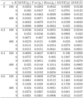
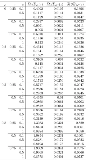
2.1 Monte Carlo MSE, Variance and Bias . . . 48
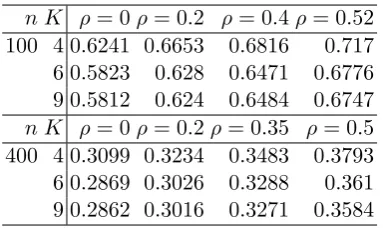
2.2 Monte Carlo average 95 % CI length . . . 48
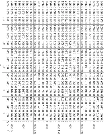
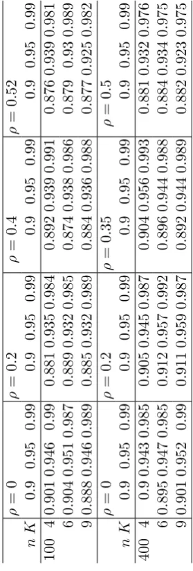
2.3 Coverage Probabilities . . . 49
2.4 Empirical power of 95% test,K = 6 . . . 50
2.5 Monte Carlo MSE, Variance and Bias . . . 51
2.6 Monte Carlo average 95 % CI length . . . 51
2.7 Coverage Probabilities . . . 52
2.8 Empirical power of 95% test . . . 52
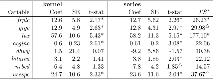
2.9 Hedonic House Pricing . . . 54
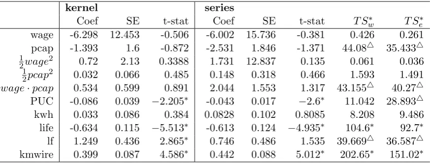
2.10 Cost function in Electricity Distribution . . . 55
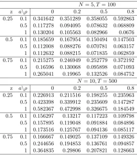
3.1 Monte Carlo MSE, N = 5, T = 100 . . . 97
3.2 Monte Carlo MSE, N = 10, T = 500 . . . 98
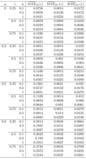
3.3 Relative MSE:M SE( ˜m∗(z))/M SE( ˜m(z)) . . . 99
3.4 Relative MSE:M SE( ˆm∗(z))/M SE( ˜m(z)) . . . 99
4.1 Relative Monte Carlo Variance,V ar(ˆλ)/V ar(˜λQM LE) . . . 144
1
Introduction
This chapter provides an overview of the motivations for, and contributions of,
the present thesis. A review of relevant literature on the topics of cross-sectional dependence and non- and semi-parametric methods is provided in detail, in order to
help place the thesis in perspective. We then summarise the main contributions of
each of the three topics of this thesis in relation to the existing studies.
1.1 Cross-sectional dependence
Three types of data are encountered in economics, namely, time series, cross-section
and panel data. This thesis focuses on estimation and inference for the latter two types and consists of three chapters developing non- and semi-parametric methods that
either allow for or estimate cross-sectional dependence in the disturbance terms of a
regression model. Implications of possible dependence between cross-sectional units on econometric methods has been less studied in the literature than that of dependence
across time periods. Unfortunately, the nature of cross-sectional dependence and
heterogeneity observed in economic data hinders a simple extension of the time series literature to cross-section or panel data.
In economic datasets, cross-sectional units naturally correspond to economic
en-tities, such as individuals, households, firms, industries, cities, regions or countries. A typical type of dataset involving smaller units like individuals or households
con-sists of survey data collected by governments or firms using various sampling schemes.
The most prevalent sampling schemes encountered in economics are simple random sampling where each unit has the same probability of being sampled, cluster
sam-pling where clusters consisting of individual units are sampled, or stratified samsam-pling
where units in the sample are represented with different frequencies than they are in the population, see Wooldridge (2002, pp. 132-135) for a good exposition. When
the cross-section units are larger entities such as firms within an industry, regions
or countries, the sampling may be exhaustive, i.e. all population units are observed in the data. It is obvious that the need to allow for dependence and heterogeneity
across cross sectional units is even more compelling when the sample coincides with
the population.
A standard practice in the econometric literature, particularly with survey data,
has been to assume that cross-sectional observations are independent and identically distributed (i.i.d.). An exception to this is the literature on data collected using
clus-ter sampling, where accounting for possible group effects via clusclus-ter-robust standard
errors of Liang and Zeger (1986) is widely available. This method allows for arbitrary dependence within clusters but assumes independence between clusters and works well
when the number of clusters is large relative to the sample size. There seems to be
partly explains the relative lack of econometric literature concerning cross-sectional
dependence in survey data. In the case of larger cross-sectional units, there has been relatively more literature that allows for cross-sectional dependence, as will be
dis-cussed below.
In the case of survey data, it is important to appreciate that when there is depen-dence and heterogeneity between underlying cross-sectional units in the population,
thei.i.dassumption on the sampled units is at best an approximation, that needs to be carefully weighed against the specific data setting under consideration. Even the simple random sampling scheme does not warrant that the sampled units are i.i.d., as clearly exposited in Andrews (2005) and Conley (1999). They offer probabilistic
frameworks which first define random vectors for all units in the population, not just the observed units, and then consider drawing sampled units from the population.
There are two possible sources of dependence in the error terms of cross
sec-tional units that have been discussed in the econometric literature. Firstly, there may be common shocks that affect all or some of individual units. Andrews (2003)
gives a comprehensive discussion on possible common shocks that may arise in
eco-nomic contexts, such as macroecoeco-nomic, technological, legal/institutional, political, environmental, health and sociological shocks. Such shocks could have either global
or local effects, influencing individual units in a possibly heterogeneous manner, that
may depend on the unit’s characteristics. Secondly, there may be dependence between individual units’ unobservables due to their economic interactions. Conley (1999)
pro-vides an example where insurance contracts are made by risk-averse agents in order to smooth individual idiosyncratic shocks. This inevitably leads to dependence in
con-sumption across those individuals. Another example arises due to spill-over between
agents: an idiosyncratic productivity shock to a firm/industry, such as technological innovation, may subsequently affect the productivity of other related firms/industries.
Yet another example arises in hedonic pricing model of houses: neighbouring houses
may share similar unobservable characteristics resulting in spatial dependence in the disturbance terms, although this example does not arise from economic interaction as
such. In these three examples, it is clear that such dependence will be governed by
the degree of interaction/proximity between units. Dependence arising from economic interaction is likely to be local in nature, in contrast to that generated by the presence
of common shocks, which can produce either global or local effects.
1.1.1 Models of cross-sectional dependence in disturbance terms
Models with common shocks
For the case of common shocks, recent works by Bai (2009) and Pesaran (2006)
consider the linear regression model with large N, large T panel data. They model the error term of the i-th cross sectional unit’st-th time period observation as, Uit=
λ0iFt +εit, where Ft is the vector of unobserved common factors, λi the vector of
individual-specific factor loadings, giving rise to cross-sectional dependence, and εit
the idiosyncratic error. Both papers allows the unobserved factors, Ft, to also affect
the regressors linearly, which seems plausible especially in macroeconomic settings
such as cross-country data, for which the largeN and large T asymptotic framework of the papers is particularly relevant as N and T may be of similar magnitude. This however results in the componentλ0iFtin the error terms that are correlated with the
regressors, which can be seen as individual-specific and time-varying ”fixed effects”
that cannot be purged by simple data transformation like first differencing. The two papers provide estimation methods that lead to consistent estimates of the linear
parameters of the regression model despite the presence of such fixed effects. The
estimation methods of the above papers are unfortunately not applicable to cross-section data and it is not straightforward to extend similar methods to nonlinear
or non- and semi-parametric regression models or to relax the linear specification in
which the unobserved factors affect the disturbance term and/or regressor.
Andrews (2005) looks at the linear regression model with cross-section data when
there is arbitrary dependence and heterogeneity in the error terms between underlying
units in population generated by the presence of common shocks, and observations are collected using random sampling. He derives asymptotic properties of the least
squares (LS) estimates of the linear parameters of the regression and establishes a nec-essary and sufficient condition for consistency. This condition requires the regressors
and errors to be uncorrelated conditional on the σ-field, C, generated by the com-mon shocks. The random sampling assumption implies that observations are i.i.d. conditional on C, needed for law of large numbers (LLN) and central limit theorem (CLT) results that are used to show asymptotic properties of the LS estimate. The
asymptotic framework offered by Andrews (2005) is indeed very useful for survey data collected using random sampling schemes but not when random sampling does not
hold.
Spatial models
For cross-sectional dependence in the unobservables arising from economic agents’ interdependence, two classes of models of dependence have been prominent in recent
literature, involving a concept of ”economic location”. As mentioned above,
cross-sectional units in economic data correspond to economic agents such as individuals or firms. One could envisage that these agents are positioned in some socio-economic
(even geographical) space, whereby their relative locations in this space underpin the
The first type of model includes the pure Spatial Autoregressive (SAR) and related
models, which form a part of a more general class of models, first suggested by Cliff and Ord (1968). This class of models is characterized by the use of exogenously given
weight matrices, which capture the structure of spatial dependence between units
up to a finite number of unknown parameters. In the case of modelling dependence in the error terms, the spatial dependence is simply modelled parametrically as a
linear transformation of underlying shocks. Let U = (U1,· · · , Un)0 be a vector of
observations having zero mean, with the prime denoting transposition. The class of spatial dependence models is given by
Q(λ0)U =σ0ε, (1.1.1)
whereε= (ε1,· · · , εn)0 is a vector ofi.i.d. random variables with zero mean and unit
variance,σ0 is a scalar,λ0 is a finite-dimensional vector of parameters, andQ(λ0) is a
known, non-singular n×nmatrix function of its argument. In general λ0, µ0 and σ0
are unknown and Q depends on one or more known spatial weight matrices. Denote by W a genericn×nmatrix,with real-valued elements wij such that
wii= 0,
n X
j=1
wij = 1, i= 1,· · · , n. (1.1.2)
The latter condition, called row normalization restriction, is not always imposed in
the literature, but some normalization on W is required in order to identify λ0. The
quantities wij are typically interpreted as inverse economic distances, see e.g. Arbia
(2006), and may form triangular arrays. The following are three examples of Q in which λ0 is scalar:
1. Pure SAR(1) (spatial autoregression of degree 1)
Q(λ0) =I−λ0W, (1.1.3)
whereI is the n×nidentity matrix andλ0 ∈(−1,1).
2. Pure SMA(1) (spatial moving average of degree 1)
Q(λ0) = (I−λ0W)−1,
forλ0∈(−1,1).
3. MESS (matrix spatial exponential, see LeSage and Pace (2009)):
The clear limitation of these models is the presumption that the spatial dependence is known to the practitioner up to a small number of parameters (λ0). Nonetheless,
these models, the pure SAR model in particular, have gained popularity in empirical
works, see Arbia (2006) for examples. In these models where the spatial dependence is parsimoniously captured by the unknownλ0, the estimation ofλ0 is often of interest,
possibly for the purpose of testing for lack of spatial dependence. In chapter 3 of the
thesis, efficient estimation ofλ0 in a generalised version of (1.1.3) is considered.
The second class of models involves the use of mixing coefficients familiar from
the time series literature. Suppose unit i is endowed with a vector of characteristics zi, the economic distance between units i and j is defined as the distance between
zi and zj, e.g. the Euclidean norm kzi−zjk. Conley (1999) approximates the
lo-cations zi by regularly spaced lattice points and applies strong mixing conditions in
deriving asymptotic theory for generalized method of moments (GMM) estimates. An alternative mixing condition in spatial setting was proposed in Pinkse, Shen and
Slade (2007). Mixing conditions, in contrast to the SAR and related models
men-tioned above, are essentially non-parametric, desirably avoiding a specific parametric description of dependence.
It is notable that in the models with common factors, cross-sectional dependence
is allowed to be ”strong” as well as ”weak”, in the sense that common shocks are al-lowed to affect all units in the sample (and population) significantly. In contrast,
the afore-mentioned spatial models require spatial dependence to fall as the
eco-nomic distance between units increases, sufficiently fast that the strength of spatial-dependence satisfies weak spatial-dependence conditions analogous to ones in time series
literature. For this thesis, the ”weak” dependence in Ui is defined by the condition n
X
i,j=1
|Cov(Ui, Uj)|=O(n), which is analogous to the concept of weak dependence in
stationary time series:
∞
X
k=−∞
|Cov(U1, U1+k)| < ∞. ”Strong” dependence in Ui, on
the other hand, is defined by the condition
n X
i,j=1
|Cov(Ui, Uj)|/n→ ∞ asn→ ∞. In
Chapter 4, it is explained how the existing SAR literature imposes weak dependence
restriction. In the case of weak dependence, the common factor models and spatial models may produce similar patterns of dependence, although the motivation and
specification of the disturbance terms may be rather different.
Model of Robinson (2011)
Robinson (2011) provides an alternative way of modeling cross-sectional depen-dence, which can produce strong as well as weak dependepen-dence, and need not involve
known economic distances although can readily accommodate them. The following
Ui =σi(Xi)ei, ei = X
j=1
bijεj, X
j=1
b2ij = 1, 1≤i≤n, n= 1,2,· · · , (1.1.4)
whereUi is the scalar disturbance term,Xi a finite dimensional vector of regressors in
the regression model,εj’s are independent random variables with zero mean and unit
variance that are independent of {Xi, i = 1,· · · , n, n ≥ 1}, σi’s are scalar unknown
functions and bij’s are unknown fixed weights. These weights bij’s, and hence Ui’s,
may form triangular arrays, and the reference tonis suppressed for ease of notation. Notice thatei’s are generated by summation overj= 1 to infinity, letting the sampled
units be also affected by unsampled units, in contrast to the pure SAR and related
models. This specification allows both unconditional and conditional heteroscedas-ticity. The triangular array structure also accommodates the panel data case where
some relabeling of observations would be required if both T and N are allowed to grow as n = N T → ∞. As the unknown weights bij’s may vary across i and j, the
above specification offers a general model of spatial dependence.
An important question to ask when specifying the model for the disturbance in
a regression with stochastic regressors is the extent to which the disturbance term is dependent with the regressors. Pesaran (2006) and Bai (2009) allow the same set
of unobserved factors to enter both regressors and error terms, and Andrews (2005) requires that they are uncorrelated conditional on theσ-algebra of common shocks. In comparison, the above specification is relatively more restrictive in thatei is
indepen-dent of the regressors Xi’s. In particular, one may be concerned that the dependence
patterns between unitsi and kin their disturbance terms and the regressors may be similar, especially in the spatial setting where they may be governed by the same
dis-tance measure between the units. The specification (1.1.4) does allow the dependence between unitsiand k in regressors and disturbances to be related. For example, one could let the joint density function fik of Xi and Xk, which reflects the dependence
between two units’ regressors, be a function of a distance between unit i and k, de-noteddik, i.e. fik(x, y) =f(x, y;dik) and at the same time also allow the weightsbik’s
to be governed by the same distance measure, bik =b(dik).
1.1.2 Some implications of cross-sectional dependence
The consequence of cross-sectional dependence in estimation of a regression model varies according to the strength of dependence. It has been shown in the time series
literature that weak dependence typically does not affect consistency or asymptotic
normality results of parameter estimates, but does alter their variances relative to the i.i.d.setting. Therefore disturbance variance structures need to be suitably estimated in order to carry out valid inference. In case of strong dependence, depending on
afore-mentioned papers that allow for strong dependence (Andrews (2005) and Robinson (2011)), consistency and asymptotic normality of estimates were shown under suitable
conditions. The issues discussed in Pesaran (2006) and Bai (2009) are rather different
as there is the additional problem of correlation between regressors and disturbance terms and the two papers offer new methods of estimation that achieve consistency of
regression parameter estimates.
Developing standard errors that are robust to dependence and heterogeneity is considerably more difficult in the cross-sectional setting than in time series, where so
called heteroscedasticity autocorrelation consistent (HAC) estimation is facilitated by
the information carried by the time index. The dependence between observations at times t and s is modelled in terms of |t−s|. In the spatial context, an extension of HAC estimation is feasible if additional information which may take the role of
the time indices is available e.g. the socio-economic or geographical distance between units which underpin the structure of the spatial dependence. Conley (1999) has
considered HAC estimation under a stationary random field with measurement error
in distance measures, Kelejian and Prucha (2007) for models of Cliff and Ord (1968) and Robinson and Thawornkaiwong (2010) for a more general set-up than Cliff-Ord
type models. Chapter 1 of this thesis offers an alternative method of robust inference
to that based on HAC estimation.
1.2 Non- and semi-parametric methods in economics
In the afore-mentioned papers, regression models take a parametric form, with the
exception of Robinson (2011). However economic theory usually does not imply a particular functional form and there may be little confidence that a linear or specific
nonlinear regression model is correctly specified. Non-parametric estimation allow
researchers to drop the presumption of known functional form, instead requiring non-parametric restrictions such as smoothness and existence of certain moments, that
may be less restrictive. In some contexts, specifying some components of the model to
be parametric while keeping the others non-parametric may be more appealing than a fully non-parametric specification. This could be either due to practical reasons, such
as avoiding ”curse of dimensionality” in non-parametric regression with many
regres-sors, or due to the practitioner having confidence and interest in parameterization of some components while not in the others. Such models are called semi-parametric.
Chapter 2 consider estimation of known functionals of the non-parametric regression function, an example of which is estimation of slope parameters in partly linear re-gression model, in which some regressors enter linearly and others non-parametrically.
In Chapter 4, the regression model is parametric but the unknown error density is left to be non-parametric. A non-parametric estimate of the ”score” function, the
ratio of the first derivative of the error density to the density itself, is used in order
for non-parametric and semi-parametric estimates. Non-parametric estimates achieve
a slower rate of convergence to the true value, compared to the correctly specified parametric estimates, which is a natural consequence of the parsimony of the latter.
In contrast, some semi-parametric estimates have been shown to achieve the same
rate of convergence as its parametric counterpart under suitable conditions, which is remarkable since semi-parametric estimates rely on the first stage non-parametric
estimates that exhibit a slower rate of convergence. This type of results has received
wide interest in econometric literature, starting from Robinson (1988) and Powell, Stock and Stocker (1989), which deal with the two well-known semi-parametric models,
partly linear regression model and single index model, respectively. Chapter 2 of
this thesis provides a set of sufficient conditions, including those on the strength of dependence and heterogeneity in the data, for semi-parametric estimates to obtain
the parametric rate of convergence.
There are two main methods of non- and semi-parametric estimation used in econometrics. The first method is the kernel approach, which uses local
smooth-ing/averaging with a chosen kernel function and bandwidth parameter. The second
is the sieve estimation method, which uses an increasing number of base functions as the sample size increases, to approximate the non-parametric function of interest. In
this thesis, the focus is on estimation of the conditional expectation, i.e. regression
function, which is the topic of the first two chapters, and the score function used in the third chapter is estimated using the same method as regression estimation. In the
sieve estimation literature, regression estimation has been developed under the name of series estimation and in the context of this thesis, the terms ”sieve” and ”series”
are used interchangeably.
There are many theoretical results on kernel estimation of regression and density under temporal dependence, see e.g. Roussas (1969), Rosenblatt (1971), Robinson
(1983) for weak dependence and Robinson (1991), Robinson (1997), Hidalgo (1997)
for strong dependence. A notable difference from parametric estimation is that in the case of weak dependence, the asymptotic variance of non-parametric kernel estimates
are the same as in the i.i.d. setting, which arises from the local nature of estimation. Robinson (2011) and Robinson and Thawornkaiwong (2010) have considered kernel estimation in non-parametric regression and partly linear regression, respectively,
un-der strong and weak cross-sectional dependence and found similar results to the time
series literature.
The main advantages of series estimation over kernel estimation are four-fold.
When economic theory generates certain restrictions on the non-parametric function
of interest, such as monotonicity, convexity and additive separability, series estimation offers a more natural way of using such information in estimation by reflecting it in
the data is summarized by a relatively few estimated coefficients. Thirdly, from a theoretical point of view, theories can be developed in a unified way to include both
non-parametric regression and general semi-parametric quantities, as will be made
clear in Chapter 2. This is in contrast to kernel estimation where an asymptotic theory for each semi-parametric model needs to be developed separately. Finally,
semi-parametric estimation with kernel methods typically involves ”trimming” out
some observations, if the density estimates at their values are smaller than a certain trimming parameter. This is because of the form of many kernel estimates which have
as their denominator, the random density estimate that can be very close to zero.
Introduction of a user-chosen trimming-parameter could be in itself a disincentive to the practitioner, while generating complications in development of econometric theory
behind estimation. Semi-parametric estimation of series method is free from the need
for trimming.
The asymptotic behaviour of series estimation under independence has been
stud-ied in Andrews (1991) and Newey (1997). For weakly dependent time series data,
Chen and Shen (1998) and Chen, Liao and Sun (2011) together offer asymptotic theory and robust inference of general sieve M estimation, which includes series
esti-mation as a special case. Importantly, Chen, Liao and Sun (2011) found that certain
non-parametric sieve estimates under weak temporal dependence also have the same asymptotic variance as in thei.i.d.setting, analogous to the result reported for kernel estimation in Robinson (1983). Chapter 2 of this thesis establishes asymptotic theory
for a spatial setting similar to Robinson (2011), which covers strong, as well as weak, dependence. In future work, it would be of interest to extend Chen et al. (2007)’s finding to the spatial setting and compare asymptotic results on series estimates of non-parametric regression to those of kernel estimates, reported in Robinson (2011).
1.3 Summary of main contributions
This section highlights the contributions of each of the three chapters of this thesis,
and place them in relation to the existing studies.
1.3.1 Chapter 2
In Chapter 2 ”Series estimation under cross-sectional dependence”, the following
model is studied,
Yi =m(Xi) +Ui, where Ui=σ(Xi)ei,
ei =
∞
X
j=1
bijεj, sup i
∞
X
j=1
b2ij <∞, 1≤i≤n, n= 1,2,· · · ,
con-The specification of Ui has been slightly modified from Robinson (2011), but both
conditional and unconditional heteroscedasticities are still allowed.
The quantity of interest is ad×1 functional ofmdenotedθ0 =a(m), which is
esti-mated by plugging in the series estimate ˆmofmin the known functional operatora(·). Theorem 2.1 reports a uniform rate of convergence of ˆmtom. A uniform rate of con-vergence for non-parametric regression estimates is useful for many semi-parametric
problems and has been extensively studied in the context of kernel estimation, see e.g.
Masry (1996) and Hansen (2008). For series estimation, Newey (1997) provided a rate for the i.i.d. setting, which was subsequently improved by de Jong (2002), under the additional assumption of compactX. The rate result obtained in Theorem 2.1 reduces to that of Newey (1997) under the i.i.d. setting and contains a variance contribution term that reflects the collective dependence in theUi’s andXi’s.
In this work, dependence in{Xi}is allowed to be strong, as well as weak, and two
measures of dependence are introduced. The first is used in showing the consistency and CLT results, while the second is needed for the variance matrix of the estimate ˆ
θ=a( ˆm) conditional on{Xi}to be well-behaved so that the unconditional asymptotic
variance matrix can be obtained. The first measure of dependence is defined in terms of departure of bivariate density function from the product of marginals. Denote by
fij the joint density function of Xi and Xj and define,
4n:=
n X
i,j=1,i6=j Z
X2
|fij(x, y)−f(x)f(y)|dxdy.
The rate of growth of4nis a measure of bi-variate dependence in theXi’s and has an
upper bound of 2n2. The quantity4n is zero in case of independence acrossiand we
may view the condition 4n =O(n) as an analogue to short-range/weak dependence in the time series literature. We find an upper bound on4nfor the case of Gaussian
Xi’s to be n X
i,j=1,i6=j
|Cov(Xi, Xj)|, which is the quantity used in the definition of weak
dependence earlier.
Similar measures of dependence have been used in Robinson (2011), where the local
nature of kernel estimation meant conditions were confined to the neighbourhoods
of the points at which the function m was estimated. For establishing asymptotic normality result for kernel estimates of m, Robinson (2011) also imposed conditions on the third and fourth order joint probability densities ofXi.
For the partly linear regression model, Robinson and Thawornkaiwong (2010) also offered a global measure of dependence which involves the supremum over the entire
support ofXi. However, the measures of dependence used in their Assumption B6 are
of marginal and joint densities of order up to four. We avoid imposing restrictions on the third and fourth order joint densities of Xi’s, which are considerably harder
to verify than that involving bivariate density even in the simple case of Gaussian
random variables. Instead we formulate our second measure of dependence in {Xi}
in terms of the fourth order cumulants of quantities combining Ui and Xi. Our
re-strictions on their collective dependence allow strong, as well as weak dependence in
both Xi’s andUi’s. Cumulants have been often used in the time series literature as a
measure of dependence, see e.g. Brillinger (1981). Chapter 2 also provides sufficient
conditions for ˆθ = a( ˆm) of certain smooth functionals a(·) to be √n-consistent, ex-tending Newey (1997)’s results obtained in thei.i.dsetting. It is interesting that some strong dependence inXi is allowed although theUi’s need to be weakly dependent for
the√n-consistency result.
Chapter 2 of this thesis also establishes theoretical justification for the use of the studentization method of Kiefer, Vogelsang and Bunzel (2000), which is new to the
cross-sectional setting and non- and semi-parametric methods. In time series, HAC
estimation of the asymptotic variance matrix is widely known to perform poorly in small samples, see e.g. Andrews and Monahan (1992) and Den Haan and Levin
(1997). Kiefer et al. (2000) offer a data-driven studentization method that can produce better small sample performance than HAC-based inference. Kiefer et al. (2000)’s assumption A1 requires a functional central limit theorem (FCLT) result on
a data-driven quantity that forms a basis of the studentizing matrix. They provide
conditions of Phillips and Durlauf (1986) as an example of a set of sufficient conditions for this FCLT result to hold. Phillips and Durlauf (1986)’s conditions require weakly
stationary α-mixing sequences. The contributions of the extensions offered by the current thesis are as follows.
1) This is the first work to apply Kiefer et al. (2000)’s studentization method in non- and/or semi-parametric contexts to the best of our knowledge.
2) We relax the conditions of homogeneity, regular spacing and ordering of Ui’s
and Xi’s, which are exhibited by stationary time series, but not by cross-sectional
data.
Indeed, a notable contribution of Chapter 2 is evaluating the extent to which the
dependence and heterogeneity of theUi’s can depart from stationary mixing and still
achieve the FCLT result required in order to apply Kiefer et al. (2000)’s studentiza-tion method. The degree of relaxastudentiza-tion of the regularity condistudentiza-tions is summarised by
Assumption C3 of Chapter 2, where a detailed discussion can also be found.
The main results of Chapter 2 are, Theorem 2.1 which states the uniform rate of convergence for the series regression estimate, Theorem 2.2 that presents the
asymp-totic distribution of the estimate of a functional of the regression function, and
fixed effects”, considers the following model for a balanced panel data set of sizeN×T. Below Yit denotes a one dimensional dependent variable, λi an additive
individual-specific fixed effect of individual i, Zt is a vector of time-varying regressor common
to all individuals, whereas m(·) is the non-parametric regression function of interest, and Uit denotes the error term:
Yit=λi+m(Zt) +Uit, E(UtUt0|Zt=z) = Ω(z), i= 1,· · ·, N, t= 1,· · ·, T,
where Ω(·) is a N ×N matrix of smooth functions. Importantly, an arbitrary form and strength of cross-sectional dependence are allowed in Uit, while Zt and Uit’s are
required to satisfy a β-mixing condition over time. Nadaraya-Watson (N-W) kernel estimate is used to estimate m(·). The setting in mind is with largerT thanN, such as in regional data with long time series. Cross-sectional units are typically large
entities like regions or countries in such settings, where the need to allow for strong dependence and heterogeneity across the cross-section may be compelling. Therefore
we do not impose restrictions on Ω, other than some smoothness and boundedness
conditions.
A similar model was considered in Robinson (2011) in the context of common
trend estimation, with Zt replaced by the deterministic argument t/T where Uit’s
are assumed to be i.i.d. across time. He clarified the issue of joint identification of m(·) and λi’s and showed how to incorporate the knowledge of cross-sectional
dependence in Uit’s into estimating m(t/T) in order to obtain an efficiency gain. In
particular, a generalised least squares (GLS) type estimate under the full knowledge of cross-sectional dependence was shown to be superior in the mean square error (MSE)
sense, to the one that does not incorporate such information. Asymptotic equivalence
between the infeasible and feasible GLS type estimates was also established.
Chapter 3 of this thesis essentially extends the results of Robinson (2011) to the
case of multivariate non-stochastic regressor, which leads to the need for conditional
heteroscedasticity captured in Ω(z). We also allow Zt and Uit’s to be jointly weakly
dependent over time, rather than using thei.i.d.condition imposed onUit’s in
Robin-son (2011). We first establish asymptotic MSE, the consequent optimal bandwidth choice and asymptotic distribution of a simple N-W estimate of m(·) based on the simple cross-sectional average of Yit’s,
n X
i=1
Yit/n. We then obtain similar results for
the optimal N-W estimate, based on the knowledge of the cross-sectional error
covari-ance structure Ω. This optimal estimate is analogous to the GLS estimate in linear
regression model where a data transformation based on Ω produces transformed er-ror terms that are homoscedastic and uncorrelated. A similar principle is used here,
con-struct a feasible version of such optimal estimate using an estimate of Ω based on the fitted residuals from the simple N-W estimation. We establish asymptotic equivalence
between the feasible and infeasible versions of the optimal N-W estimate and also
between their optimal bandwidth choices. Unlike in Robinson (2011), the conditional heteroscedasticity here implies that the optimal weight for the GLS-type estimation
now varies over the pointz at which the functionm(·) is estimated.
In obtaining the theoretical results, we prove a useful result, Lemma 3.6, that represents an additional and significant contribution of the chapter. Many sample
quantities in econometrics take the form of a U-statistic, whose properties in thei.i.d. setting are well understood. Similar results on the behaviour of U-statistics under dependence is often obtained by showing the negligibility of the departure of the
U-statistic under dependent process from its counterpart under thei.i.d.setting. Dehling (2006) offers an excellent review of both the literature under thei.i.d.setting and that covering the dependent case. Fan and Li (1999) utilized Yoshihara (1976)’s lemma, to
obtain an upper bound on the difference in expectations of a third order U-statistic
under independence and the β-mixing process. Lemma 3.6 of this chapter extends Fan and Li (1999)’s result to U-statistics with an asymmetric kernel and of order up
to four. This lemma would be useful in many applications, especially when finding
the asymptotic order of magnitude for moments of various estimates with time series data.
The main results of Chapter 3 are, Theorem 3.7 which establishes how good an
estimate of the cross-sectional error covariance matrix we have, and Lemma 3.6 that presents useful decomposition of the expectation of U-statistics based on β-mixing processes.
1.3.3 Chapter 4
While Chapters 2 and 3 deal with non-parametric regression models, in Chapter 4 ”Efficiency improvement in the semi-parametric pure Spatial Autoregressive (SAR)
model”, we consider the parametric pure SAR model, presented in (1.1.1) and (1.1.3).
We state the model again for ease of reference:
(I−λ0W)U =σ0ε. (1.3.1)
For the weight matrix W, it is assumed that max
1≤i,j≤n|wij|=O(1/h), with a sequence
h=hnthat is either fixed or divergent asn→ ∞. This is a typical condition imposed
in the SAR literature, e.g. in Lee (2002, 2004), Kelejian and Prucha (1998), and it
has been shown that the behaviour of the sequenceh has implications on asymptotic theory of parameter estimates. In Chapter 4, Ui will be allowed to have a non-zero
mean, providing a model for observables, as well as disturbances. However for clarity
to be consistent, at the usual rate n when h is fixed, and at a slower rate, pn/h, if h is divergent. When εj’s, therefore Ui’s, are Gaussian, the Gaussian PMLE is of
course the MLE itself, attaining the Cramer-Rao bound. This property is lost once the
true likelihood seizes to be Gaussian. The lack of efficiency property of the Gaussian
PMLE of λ0 when Ui’s are not Gaussian, in addition to the possibly slower rate of
convergence in case of divergent h, gives rise to an interest in improved estimation of λ0. This is the focus of Chapter 4 and we treatµ0 and σ0 as nuisance parameters.
We let εi’s be i.i.d. with unknown density function of non-parametric form, thus
avoiding possible parametric misspecification of density function, which could lead
to inconsistency of the corresponding MLE. This is what makes the model
semi-parametric, as it contains a non-parametric error density function along with a para-metric regression model. There is a large literature addressing whether the
Cramer-Rao bound of the correctly specified MLE can be achieved in the absence of knowledge
of the density function, with only non-parametric assumptions. This is attained by an estimate that takes an approximate Newton-step from an initial consistent and
ineffi-cient estimate ofλ0, which is the Gaussian PMLE in our case. In Beran (1976), Newey
(1988), Robinson (1995) and Robinson (2011), the Newton-step is constructed from a non-parametric series estimate of the score function of the error density. Chapter 4
also uses this estimate and establishes that it indeed achieves the Cramer-Rao bound
of the correctly specified MLE.
Another notable and interesting finding of Chapter 4 is that the relative efficiency
of the adaptive estimate ˆλ to the PMLE can be either less or more than ones in the classical outcome, which includes the results under mixed regressive SAR model
considered in Robinson (2011) and the time series setting. As mentioned earlier, pure
SAR model is a particularly popular model in the more general class of models and it is hoped that the results of this chapter may be extended in future to other models.
The main results of Chapter 4 are, Lemma 4.1 which establishes feasibility of
efficiency improvement from the (Gaussian) PMLE of λ0, and Theorem 4.1 which
presents the asymptotic distribution of the improved estimate, which coincides with
2
Series Estimation under
Cross-sectional Dependence
2.1 Introduction
Economic agents are typically interdependent, due for example to externalities,
spill-overs or the presence of common shocks. Such dependence is often overlooked in
cross-sectional or panel data analysis, in part due to a lack of econometric literature that deals with the issue at hand. Implications of dependence on econometric analysis have
long been studied in the context of time series data, where the temporal dependence
is naturally modeled in terms of the distance between observations along the time axis. Unfortunately, the nature of cross-sectional dependence observed in economic
data hinders a simple multi-dimensional extension of time series literature to spatial
data. For example, the index of observations in economic cross-sectional data cannot be used to describe the dependence between units in the way that the time index can
be. This is because there is often no natural ordering of cross-sectional data and the
indices do not represent relative positioning of the units sampled.
In order to start accounting for possible cross-sectional dependence, one needs
first to establish a framework under which the structure of such dependence can be suitably formalised. Three classes of models of cross-sectional dependence have been
prominent in recent literature. The first class of models deal with the presence of
unobserved common factors that may affect some/all of individual units, see Andrews (2005), Pesaran (2006) and Bai (2005). These models could give rise to cross-sectional
dependence that are persistent throughout units, analogous to ”strong” or
”long-range” dependence in the time series literature.
The other two classes of models involve a concept of ”economic location”. In
economic data, cross-sectional units correspond to economic agents such as individuals
or firms. One could envisage that these agents are positioned in some socio-economic (even geographical) space, whereby their relative locations in this space underpin the
strength of dependence between them. For a detailed discussion and examples of such
proximity, see e.g. Conley (1999) and Pinkse, Slade and Brett (2002).
The second class of models is the Spatial Autoregressive (SAR) model of Cliff and
Ord (1968, 1981), see e.g. Lee (2002, 2004), Kelejian and Prucha (1998, 1999),
Robin-son (2010a), Rossi (2010). In this approach, the dependent variable (or disturbance) of a given unit is assumed to be affected by a weighted average of the dependent
vari-ables (or disturbances) of the other sampled units. The weights used in the averaging
are presumed to be known and reflect the degree of proximity between agents, leaving a finite number of parameters (often scalar) to be estimated to explain the spatial
dependence. The SAR model has gained popularity in empirical works, see e.g. Arbia
conditions in terms of economic distance between agents, under a suitable stationarity
assumption. An alternative mixing condition in spatial setting was proposed in Pinkse, Shen and Slade (2007).
Robinson (2011) has offered a new way of modeling cross-sectional dependence,
which doesnot hinge on the idea of economic distance although can certainly accom-modate it. A general, possibly non-stationary, linear process is assumed for
distur-bances, which, unlike a mixing framework, allows possible strong dependence. The
dependence in the regressors is phrased in terms of the departure of joint densities from the product of marginals, allowing possible heterogeneity across units. The model’s
ability to cover both weak and strong dependence in the error term and regressors
allows the development of a general set of theory. While the model accommodates many spatial settings plausible in economic data, no new concepts, other than those
familiar from standard econometric literature, need to be introduced.
On the other hand, non-parametric and semi-parametric estimation have become an established method in econometric analysis. Such methods allow researchers to
drop the assumption of known parametric functional form that is often not warranted
by economic theory. There are many theoretical results on non-parametric kernel estimation under temporal dependence, see e.g. Robinson (1983) and Hidalgo (1997).
Robinson (2011) and Robinson and Thawornkaiwong (2010) have considered kernel
estimation in the non-parametric regression model and the partly linear regression model, respectively, under cross-sectional dependence.
The asymptotic behaviour of the series estimation under independence has been studied in Andrews (1991) and Newey (1997). For weakly dependent time series
data, Chen and Shen (1998) and Chen, Liao and Sun (2011) offer a rather complete
treatment of asymptotic theory and robust inference of the general sieve M estima-tion, which includes series estimation as a special case. This chapter produces an
asymptotic theory that covers general cross-sectional heterogeneity and dependence,
including weak and strong dependence. The conditions of the chapter, while designed for spatial setting, readily lend themselves to time series and panel data, expanding
the applicability of the results to those settings. They follow the framework of
Robin-son (2011), however the nature of series estimation necessitated some modifications. This chapter offers alternative conditions in terms of the fourth order cumulants
fa-miliar from time series literature, enabling to avoid conditions on joint densities which
may be difficult to verify for some processes. Due to a number of similarities of series estimation to OLS in linear regression, asymptotic results derived here easily extend
to the linear regression.
The other main contribution of this chapter is establishing a theoretical back-ground for the use of a studentization method that offers an alternative to the
extension of HAC estimation familiar from the time series literature, see e.g. Han-nan (1957), Newey and West (1987), is possible if additional information such as
the socio-economic distance between units which underpin the structure of the
spa-tial dependence is available. Conley (1999) has considered HAC estimation under a stationary random field with measurement error in distance measures, Kelejian and
Prucha (2007) for models of Cliff and Ord (1981) and Robinson and Thawornkaiwong
(2010) for a more general set-up than Cliff-Ord type models. Bester, Conley, Hansen and Vogelsang (2008) consider the asymptotic theory of the HAC estimation when a
fixed, rather than a vanishing, proportion of the sample is used in the variance
esti-mation. However, the small sample performance of HAC estimation is known to be poor even in time series setting and an alternative method that achieves better finite
sample performance was suggested by Kiefer, Vogelsang and Bunzel (2000) in the
lin-ear regression in time series context. This chapter provides theoretical justification for extending the use of Kiefer et al.’s studentization to spatial or spatio-temporal data.
The chapter is structured as follows. In Section 2.2, the setting of the model
is outlined. In Section 2.3, the series estimation is introduced and a uniform rate of convergence for the non-parametric component is established. Section 2.4 contains
asymptotic normality results. Section 2.5 presents sufficient conditions for the√nrate of convergence of certain semi-parametric estimators, with data-driven studentization. Section 2.6 presents a small Monte Carlo study of finite sample performance. Section
2.7 discusses some empirical examples and Section 2.8 concludes. The Appendix
contains the proofs.
2.2 Setting of the model
This chapter discusses inference on the following non-parametric regression model,
Yi =m(Xi) +Ui, i= 1,2,· · · , n, (2.2.1)
where Yi, Ui ∈ R and Xi ∈ X ⊂ Rq are random variables and m : X → R is an unknown function of interest. The error term Ui of the model is assumed to follow
Ui =σ(Xi)ei, ei =
∞
X
j=1
bijεj,
∞
X
j=1
b2ij <∞ i= 1,2,· · ·, n, (2.2.2)
whereσ(·) is a real function,{bij, i, j≥1} are unknown constants and{εj, j ≥1}are independent random variables with zero mean and unit variance. Processes{Xi}and
{εj} are assumed to be independent of each other. The linear process ei in Ui was
also used in Robinson (2011) and Robinson and Thawornkaiwong (2010). Quantities
Yi, Xi, Ui, ei, εj, bij are allowed to admit a triangular structure throughout this work,
see Robinson (2011) for discussion. Allowing coefficients bij = bijn to vary with n is
important in making (2.2.2) to cover the popular SAR model, wherebyei = n X
j=1
bijnεj
will include summation only up to n.
The structure (2.2.2) is designed to encompass various forms of spatial dependence and heterogeneity in the unobserved errors Ui, that could arise in economic
applica-tions. Conditional and unconditional heteroscedasticity of the errors Ui is allowed,
while the restrictions later imposed onbij’s are rather mild, affording an ample scope
for possible non-stationarity/heterogeneity across i. For example, bij’s need not
ex-hibit any form of conformity across iand j, in particular, be affected by|i−j|. The specification (2.2.2) also accommodates the idea of ”economic distance”, in which case bij will be determined by distances between units. Restrictions on dependence and
heterogeneity inXi are stated and discussed in Section 3.
Errors (2.2.2) obviously cover equally-spaced stationary time series, where bij is
of the formb|i−j|. An alternative to (2.2.2) is a mixing framework, which would allow
us to relax the condition of independence between {Xi}ni=1 and {ei}ni=1. However, a
mixing framework necessitates the introduction of some distance measures and the notion of stationarity, which are not always justifiable in economic applications. More
importantly, long-range dependence is not covered by a mixing-framework.
Regarding the function m(x) =E(Yi|Xi =x) in (2.2.1), it denotes the conditional
expectation of Yi at Xi = x. For any given function g(·) : X → R, let a(g) denote a d×1 vector-valued functional of g(·), i.e. a mapping from a possible conditional expectation to a real vector. There are many applications where a (known) functional
a(m) of the conditional expectation m is of interest. It can be estimated by a( ˆm), where ˆm(·) denotes a series estimator of m(·), constructed as a linear combination of pre-specified approximating functions. Simple examples of a(g) include the value of the function at multiple fixed points, a(g) = (g(x1),· · · , g(xd))0, (x1,· · ·, xd) ∈ Xd,
which is of interest in non-parametric regression estimation, and the value of partial derivative of the function with respect to the `th argument at fixed points,
a(g) =∂g(x) ∂x`
x1,· · · ,
∂g(x) ∂x`
xd
0
,
which is of interest in the case of non-parametric derivative estimation. An example of
nonlinear functionala(·) given in Newey (1997) is the consumer surplus. LettingYibe
the log consumption andXi = (logpi,logIi)0, a 2×1 vector of log price and log income,
the estimated demand function at a fixed pointXi =xis given by exp( ˆm(x)), whereas
represent the lower and upper bounds on the price, is
a( ˆm) =
Z p¯ p
exp ˆm(logt,log ¯I)dt.
If one was interested in the approximate consumer surplus at multiple fixed values of
income,a( ˆm) would take a vector form. Further example of a(·) arises in the context of the partly linear regression model and will be discussed in detail in Section 5.
Previously, Andrews (1991) showed asymptotic normality for a vector-valued
lin-ear functional a( ˆm), using for {Xi}n
i=1 and {Ui}ni=1 independent and non-identically
distributed (i.n.i.d) setting and, in addition, indicating that “the proof can be ex-tended to cover strong mixing regressors without too much difficulty.” Newey (1997)
has established uniform rate of convergence for |m(x)ˆ −m(x)| and asymptotic nor-mality result for a( ˆm) −a(m) when {Xi}ni=1 and {Ui}ni=1 are both i.i.d. and a(g)
is a general (possibly nonlinear) scalar functional. Newey (1997) has also offered a
set of conditions on the functional a(·), under which a( ˆm) converges to a(m) at the parametric rate. Chen and Shen (1998) and Chen, Liao and Sun (2011) consider the problem of sieve extreme estimation for weakly dependent time series setting. In the
context of series estimation, Chen and Shen (1998)’s results yield a convergence rate
for the non-parametric regression estimate ˆm(·) and asymptotic normality for a( ˆm) in the case of √n-rate of convergece. Chen, Liao and Sun (2011) offer an asymptotic normality result that also covers the case of slower-than-√n rate of convergence and provide methods of inference robust to time series weak dependence. They also unveil a rather striking fact that for certain cases of slower-than-√nrate of convergence, the asymptotic variance of the estimate a( ˆm) coincides with that obtained under inde-pendence. An important example is the case of non-parametric regression function evaluated at a finite number of fixed points, for which a similar observation was made
by Robinson (1983) for kernel estimation.
2.3 Estimation of m and uniform consistency rate
Estimation ofm is based on the use of approximating functions. Denote byps(·), s=
1,2,· · · a set of approximating functions fromX toR:
pk(·) = (p1(·),· · ·, pk(·))0.
Next, introduce a deterministic sequence of positive integers K = Kn,
nondecreas-ing in n, which denotes the number of approximating functions used in the series estimation where n stands for the sample size. The integer K can be regarded as a bandwidth parameter, analogous to the window length in kernel estimation, and its
(Y1,· · · , Yn)0 ∈Rn,and A− denotes the Moore-Penrose inverse for a matrixA. Definition 1. A series estimator of m(x), at a fixed point x ∈ X, based on K approximating functions,pK(·) = (p
1(·),· · · , pK(·))0, is given by
ˆ
m(x) =pK(x)0β.ˆ (2.3.1)
In the remainder of this section, we establish a uniform consistency rate of the estimate ˆm(x).
Assumption A1. The random variables {Xi}ni=1, n= 1,2,· · ·, are independent of
{εj}∞j=1 and identically distributed with the probability density function f(x), x ∈ X.
The joint density of Xi and Xj, fij(x, y), x, y∈ X, exists for all i and j.
The assumption of identity of distribution on {Xi}ni=1 later facilitates proofs of
theorems by offering some algebraic simplification, allowing us to afford more hetero-geneity in the unobserved {Ui}n
i=1, which was deemed more crucial than allowing for
non-identical distribution of the observed{Xi}ni=1. Heterogeneity/non-stationarity in
Xi across iis still allowed as the dependence inXi may vary across the index i.
Assumption A2. The random variables {Ui}n
i=1, n = 1,2,· · ·, follows the linear
specification (2.2.2) with some bounded positive function σ(x) :X →R, and innova-tions {εj} are independent across j, satisfying E(ε2j) = 1 and maxj≥1 E|εj|2+ν <∞,
for some ν >0.
For any k≥1, define ak×kmatrix
Bk:=E(pk(Xi)pk(Xi)0), k= 1,2,· · ·. (2.3.2)
Let λ(A) and ¯λ(A) denote the minimal and maximal eigenvalues of a square matrix A. In this work, Euclidean norm is used for vectors: kak2 =a0a. For matrices, we use
spectral norm, induced by Euclidean vector norm: kAk = max
kxk=1
kAxk = ¯λ1/2(A0A). For functions, the uniform norm |g|∞= sup
x∈X
|g(x)|is used.
Define a sequence of scalar constants ξ(k) as
ξ(k) := sup
x∈X
kpk(x)k, k= 1,2,· · · .
Quantities similar ξ(k) were also used in Andrews (1991) and Newey (1997). If it is known that m is a bounded function, one may choose bounded and non-vanishing series functions, in which case ξ(k) increases at the rate of √k: sup
x∈X
kpk(x)k =
sup
x∈X
k X
i=1
p2i(x)1/2 ≤C √
they are B-splines.
Assumption A3. (i) There exists c >0 such that λ(Bk)≥c, ∀k≥1.
(ii) K and pK(·) are such that K2ξ4(K) =o(n).
Condition λ(Bk) ≥ c of Assumption A3(i) requires Bk to be nonsingular for all
values of k and is also assumed in Andrews (1991) and Newey (1997). When this assumption fails, some series functions in ps(·), s≥1 may be redundant and need to
be eliminated to make it hold. Assumption 3(ii) imposes an upper bound on the rate of increase of ξ(K) as K → ∞. Using the explicit bounds ξ(K) mentioned in the previous paragraph, A3 (ii) boils down to K =o(n1/4) for the case of B-splines and K = o(n1/6) in the case of orthonormal polynomials under the suitable conditions required for those expressions ofξ(K).
Assumption A4. The function m(·) : X → R and series functions ps(·), s ≥ 1,
are such that there exist a sequence of vectors βK and a number α > 0 satisfying, as
K → ∞,
|m−pK0βK|∞=O(K−α).
Assumption A4 is a standard condition used in the series estimation literature, and
appears in Andrews (1991) and Newey (1997). It requires the uniform approximation
error of m(·) by a linear combination of the chosen set of series functions to diminish fast enough. It can be seen as a smoothness condition imposed onm(·), if the functions ps(·), s = 1,2,· · · are ordered so that higher values of s correspond to less smooth
functions. In such case, the smoother the function m(·) is, the faster is the rate of decay in the coefficients of the vector βK in the series expansion pK0βK of m(·).
Some further insights into Assumption A4 for certain choices of the approximating
functions, including polynomials, trigonometric polynomials, splines and orthogonal wavelets, can be found in Chen (2007), pp. 5573. Assumption A4 will control the bias
term of our estimate ˆm, andα is also related to the number of the regressors. Newey (1997) points out that for splines and power series, Assumption A4 is satisfied with α=s/q wheresis the number of continuous derivatives of m andq is the dimension of x. Conditions imposing an upper bound on the rate of increase in K, such as A3 (ii), may necessitate a stronger assumption on the smoothness of the unknownm.
Now, we will state an assumption that is required to control the strength of
de-pendence in Xi’s across i. Introduce the quantity:
4n:= n X
i,j=1,i6=j Z
X2
|fij(x, y)−f(x)f(y)|dxdy. (2.3.3)
The rate of growth of 4n is a measure of bi-variate dependence in Xi’s and has
an upper bound of 2n2, a useful property used in the proofs. The quantity 4n is zero in case of independence across i and we may view the condition 4n = O(n)
as an analogue to the concept of short-range/weak dependence in time series
simple bound. Letσij(X) :=Cov(Xi, Xj). Assume for simplicity thatσii(X)=σ
(X)
i = 1.
If for somec0<1, one has |σ(ikX)| ≤c0,∀i, k = 1,· · · , n;i6=k, n≥1, then
4n ≤C
n X
i,k=1,i6=k
|σik(X)|, n≥1,
see Proposition 2.1 in Appendix B. Clearly, if max
1≤k≤n n X
i=1
|σik(X)| ≤Cn, then4n=O(n), whereas4n=o(n2) holds for a large class of covariances. Thus, in the Gaussian case,
4n can be replaced by the sum
n X
i,k=1:i6=k
|σik(X)|.
Assumption A5. Asn→ ∞,n−2K2ξ4(K)4n=o(1).
Assumption A5 indicates that stronger dependence in Xi will require the use of
smallerK. In the light of Assumption A4, this will necessitate a stronger assumption on the smoothness of the unknown function m. Under weak dependence, i.e. 4n = O(n), A5 reduces to K2ξ4(K) = o(n) which is stated in A3(ii). Otherwise, A5 is a stronger condition than A3(ii) imposed on the upper bound of the growth in K and ξ(K).
To state our first theorem, it is necessary to introduce some notation. Define
nor-malised functionsPk(x) :=Bk−1/2pk(x) withBkas in (2.3.2) such thatE(Pk(Xi)Pk(Xi)0)
=Ik. We shall writeP(x) =PK(x) withK=Kn, suppressing the superscriptK for
the rest of the chapter for the ease of notation. Note thatP(·) = [P1K(·),· · · , PKK(·)]0,
with the double subscripts at PsK(·) arising from the definition P(·) = B
−1/2
K pK(·).
Such normalised functions were also used in Newey (1997). Let P =Pn = (P(X1),
· · · , P(Xn))0 ∈ Rn×K. For a given sequence K = Kn, define the following K ×K
variance-covariance matrix Σn of the K×1 vector sum n X
i=1
P(Xi)Ui/
√ n:
Σn := E(P0U U0P/n) =V ar
1 √ n
n X
i=1
P(Xi)Ui !
(2.3.4)
= 1
n
n X
i,k=1
E P(Xi)UiUkP0(Xk)
= 1
n
n X
i,k=1
γikE(σ(Xi)σ(Xk)P(Xi)P0(Xk)),
where
γik :=Cov(
∞
X
j=1
bijεj,
∞
X
j=1
bkjεj) =
∞
X
j=1
bijbkj.
Theorem 2.1 (Uniform Rate of Convergence). Under Assumptions A1-A5,
sup
x∈X
|m(x)ˆ −m(x)|=Op ξ(K) "r
tr(Σn)
n +K
−α #!
, as n→ ∞.
This result coincides with the rate obtained by Newey (1997) fori.i.d.{Xi}and{Ui}. In the latter case Σn =σ2E(P(Xi)P(Xi)0) =σ2IK leading to tr(Σn) =O(K). The
proof of the above Theorem is given in the Appendix A. The first term in the rate of
Theorem 2.1 reflects the contribution of the variance of ˆm, while the second term arises from the bias component. The uniform rate of consistency highlights the bias/variance trade-off in the selection of K: the use of largerK reduces the bias and increases the variance.
The rates obtained in Theorem 2.1 need to be verified to be op(1), to establish
uniform consistency of the series estimate ˆm. The requirement ξ(K)K−α = o(1) of negligible bias suggests that it may be favourable to choose series functions which
are bounded. To evaluate the contribution of the variance, suppose for now that the original series functions and thus, the normalized functions P1K,· · · , PKK, are
uniformly bounded. Then, tr(Σn) =K· n X
i,k=1
γik/n, making the variance contribution
ξ(K)√K
n X
i,k=1
γik/n2 1/2
. Under weak dependence onei’s, n X
i,k=1
γik =O(n), meaning
the rate becomes ξ(K)pK/n= K/√nwhich is o(1) by Assumption A3 (ii). Under strong dependence of ei’s, the rate is slower and further conditions restricting the
increase of K and ξ(K) may be needed to show uniform consistency.
For the i.i.d. setting, the uniform rate of convergence obtained by Newey (1997) was improved by de Jong (2002), under the additional assumption of compact X. Under the presence of dependence, it was not possible to obtain improvement similar
to that achieved in de Jong (2002), whose proof makes use of Hoeffding’s inequality for a sum ofi.i.d.random variables. It would be of interest for future work to sharpen the bound provided by Theorem 2.1.
2.4 Asymptotic normality
The previous section established the uniform rate of convergence for ˆm−m, whilst our ultimate interest lies in inference on the functional a(m). Denote θ0 =a(m) and
ˆ
θ = a( ˆm). In this section, we study the asymptotic distribution of ˆθ−θ0. First,
we provide some technical assumptions needed for establishing asymptotic normality.
Recall that a(·) is a vector-valued functional operator.
Assumption B1. One of the following two assumptions holds. (i) a(g) is a linear operator ing.
(ii)For some >0, there exists a linear operatorD(g)and a constantC=C<∞