A PROPOSED METHOD OF SELECTING PAIRS OF SIFT
POINTS
MOHAMMED I. ABD-ALMAJIED1, LOAY E. GEORGE2, KAMAL M. ABOOD1
1Department of astronomy and space, College of science, University of Baghdad, Baghdad, Iraq
2Department of remote sensing and GIS, College of science, University of Baghdad, Baghdad, Iraq
ABSTRACT
Pattern matching between two scenes is an important part in image or pattern recognition and registration. It based on finding the best match between two scenes using some selected control points. Image of Solar Planets are somehow difficult in defining distinctive features for matching especially when compared with Earth’s image (ex. Contrast, resolution). Geometrical transformation (scaling and rotation) may affect the
registration due to improper selection of correct control points. The degree of distortion due to geometrical transform may affect numbers and accuracy of match. In this article, a new auto-selection method for the reference points is established. First, the scale compensation, a new procedure has evaluated for the range of scaling factor (0.5-1.5). Also, the method was established when there is a rotation effects associated with the scaling one. It was evaluated for rotation range (1o-90o) with the same range of scaling. Second, new
matching method for finding the best match between the selected list of control was introduced. This method depends on the distance and angle between corresponding points. This method tested on satellite image of Mars. A computer simulation was build using Matlab Language. The results showed a good
performance.
KEYWORDS: Sift Points, Pattern Matching, Rotation Assessment, Control Points List, Scale Assessment.
1. INTRODUCTION
The fundamental problems that are always appear that the objects in the world may display in different ways. This problem occurs when analyzing real-world measurement data [1, 2]. Many computer vision applications still tackling with, so called, invariant local features. This property is specific with set of transformations that related for detecting image features; ex. similarities or affinities [3]. The detected features from the training image is crucial for the best object recognition task [4].
Some of image matching researchers arises in the computer vision, image processing, medical imaging and remote sensing. They are precondition steps in many practical problems, such as stereo vision, object recognition, and object tracking system (ex. Camera motion images) [5, 6].
The beginning of image matching work can be back to 1981 when Moravec work on stereo matching using corner detector. It has improved by Harris and Stephens 1988 to make it appealable through small image variation and near edge [7-9].
Crowley 1981; Crowley and Parker 1984
developed a representation that specified peaks and ridges in scale space using different of Gaussian filters in tree structure; it can be used to match images with arbitrary scale change, same idea was confirmed by Lowe 1999. Laplacian of Gaussian and specific based operator were proposed by Lindeberg 1998 [1, 6, 9, 10].
some distortion in their images. The challenge of this work when find a match in images of planet. The low contrast and smooth surface of these images may affect on find a good control points between them.
The research article is organized as follows; in section 2 the relevant theoretical and steps of proposed method which represent the main area of this work. Section 3 demonstrate the implementation of this algorithm. Section 4, the test results and discussions are given, finally in section 5 is conclusions.
2. RELATED METHOD
The goal of this work is find a control points between images of the same scene for applying the image registration. The control points should be invariant to scaling and rotation. The criteria of work are by find the correct points and avoid the outliers. The smoothness and low contrast planet’s image may affect the right control points; a new robust method is adopted for this work.
2.1.Scale Invariant Feature Transform (SIFT):
Sift algorithm is a local feature detection. It detects interest points in scale space, and define their positions, scales, and rotations.
The beginning of computation is to find over all scales and image location. In scale space extreme of the difference of Gaussian function convolved with the image have been applied due to find a stable key point locations (i.e. subtracting convolved images which are adjacent in the same resolution). The main reliable work is based on Gaussian function.
The following equations represent 2-Dimensional scale space [11]:
) , ( ) , , ( ) , ,
(x y G x y I x y
L
….(1)
Where * is the convolution operator,
) , (x y
I is the image; (
) is the standard deviationof Gaussian, also, it the scale space of keypoint. The Gaussian function [9] is:
2 2 2 )/2
( 2 2 1 ) , , (
x ye y
x
G .... (2)
An extracted point selects from images filtered by Gaussian function. It is computed as the difference between two images. It passed through Gaussian function at scale k times the other one.
The D(x,y,
)is given by [4]:) , ( )) , , ( ) , , ( ( ) , ,
(x y G x y k G x y I x y
D
)
,
,
(
)
,
,
(
x
y
k
L
x
y
L
.... (3)
Each point of image is compared with its neighbors. This process continued with points of the same image but has different scale factor. The result points called sift point [5, 12].
2.2. Proximity Matrix:
This is a technique which used for finding a match between two images depend on the distance. Two points in two images consider be match when have similar locations. The corresponding between two images depends on the minimal total difference of point to point between them. Ullman was first who adopted this theory. To overcome the effect of translation, shearing, and scaling deformation, Scott and Longuet-Higgins, proposed a proximity matrix (G) by minimizing square distance between all
points defined by the formula [13-15]:
2 2 ij r ij
e
G
…. (4)Where, rij is the Euclidean distance between two
points, δ is appropriate unit of distance.
3
. METHODOLOGYdifferent artifacts that cause impact on the degree of corresponding. Scaling, rotation, instabilities of imaging system, and the different of illumination condition may affect the registration process. Image of Planet as compared to Earth satellite images, have low contrast and smooth surface area. These features establish a challenge in find a best match between images. A new method used for matching that depend on distance with its angle is established for this work.
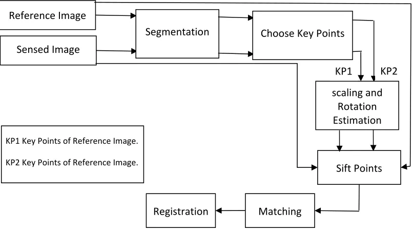
[image:3.612.113.516.260.485.2]At the first the most two operators that affect on image are scaling and rotation. For obtain best match between reference and sensed image a pre-calculation process must be done. These operation is necessary for reduce the dimensionality between these images. The effect of rotation in associated with scaling is applied on sensed image and compared with its reference one. Two algorithm have been built for estimate scaling and rotation. After that a match with registration is applied. A diagram of the operations is show in figure (1 .
Figure 1. steps of methodology.
3.1. Estimate Scale
The estimate scale is computed utilize distance measurement. The measured distances are depending on sift-points. These points need a reference point for the calculation in both images.
At first, preprocessing steps are applied on both images (reference and sensed one). The grey values range of both images were elongate through applying (standardization transform or Z-score) equation. The equation of (Z-score) is [16]:
x
x
.… (5)Where (
) represent the mean and (
) is standard deviation.Histogram is used to find the keypoints. These values are bounded to be with the range minmum and maximum in order to avoid the extrem dynamic range of brightness. This is used because sometimes suffer from brightness distortion effects. The values
Reference Image
Sensed Image
Segmentation Choose Key Points
scaling and Rotation Estimation
Sift Points
Matching Registration
KP1 KP2
KP1 Key Points of Reference Image.
of
[
',
']
Max
Min
are assessed using the following criterion [17]:
min n mi ) ( 1 I I Hist MN
0
.
02
.… (6)
max x ma ) ( 1 I I Hist MN
0
.
02
.… (7)Where
Min
'is the lowest possible value that equal equation (6)'
Max is the brightest possible value that equal
equation (7).
MN is the size of image.
The value (0.02) is a threshold value adopted to define the accepted ratio of brightness levels. This condition used in both images for obtain vaules
between ( ', '
Max Max Min
Min ).
Median filter then is used to remove the small region (island and gaps) which caused unwanted features.
[image:4.612.322.487.262.421.2]To select a specific features a distinguish between them must be used. A seed filling alogroithm was applied to set apart each one from other. A four neighbour of each pixel is depend for the seed filling as in figure (2).
Figure 2. Seed Filling tech [18].
A threshold is set for eliminate features near the edges because it is subject to some kind of distrotions. Another criteria was utilize to filter some lined features. Lined features may represent a slots, river path, and some times crack in land which is subject to various conditions through time. On the other hand, circle or semi-circle features are more consistent which is need to be establishe. A morphological operation is applied in this criteria. To detect features (circle or semi-circle), a threshold is used to check their shapes depend on the area of that features definning as:
max min
length
R
R
.… (8)max
min
width
R
R
…. (9)Where
R
min, andR
maxare:3 2 *
min R
R …. (10)
2
3
*
max
R
R
…. (11)Where R is the radius of each feature.
After that, a single feature is select from the rest that depend on its large area. Some of the enhancement is done on the selected feature by checking their brightness boundary according to the following equation:
std
V
min
*
.... (12)std
V
max
*
.... (13)Where
is the mean gray level value, std is thestandard deviation, and
is a constant (a value of 1.1 is used in this work).A center of the selected feature is compute. it is compute through the following equation [17]:
N k k i x N x 11 .… (14)
For the (y-axis) is:
N k k i y N y 11 …. (15)
Where (N) is the size of column in the (x-axis)
and the size of row in the (y-axis).
Finally, reference point represents center of the largest area of the selected feature. Distance measurement is computed using sift-points, which compute for both images using equation (1) and (2), according to reference point in both images. The estimated scale is measured using the equation [19]:
reference sensed
dis dis
Scale …. (16)
Where dis is the distance and computed as:
k dis dis k i
1 .... (17)
Where k is the no. of sift-point.
The error percentage is evaluated for this part of work using the following equation [20]:
Percentage Error *100%
OV EV OV
.... (18)
Where OV is original value, and EV evaluated
value.
3.2. Estimate Rotation
The rotation estimation was computed for the sensed image which has the scale effect as
compared to the reference image. Also, calculation of reference point is needed in this part in both images. Equations (5) to (15) were used for this work.
The center of the image with reference point is used for estimating the degree of rotation of the sensed image according to the following equation [21]:
)
(
tan
1x
y
.… (19)Percentage error was evaluated for this part by equation (18).
3.3. Estimate Match
From equation (1) and equation (2), a sift-points are compute for the both images. Two images of the same scene can find match between them according to their sift-points. The new proposed algorithm for matching is:
d
diff
…. (22)Where
d
is the difference of the distance between the match point,
is angle difference between the match point, and
is the relative diffraction of angle of points which is in the same position or diffracted some pixel from each other. The relative diffraction angle was evaluated through an equation resulted from a simulation for a pixel locate in small size window. A deflection angle is computed for three window (3*3), (5*5), and (7*7) in computer simulation.A deflection angle equation is:
2 3 4 5 6 6
9 2 10 0.0002 0.0087 0.2253
10
8 dm dm dm dm dm
983 . 23 1489
.
3
dm .… (23)
Where
d
m is the mean distance of the two points.Image registration is used for the verification of the selected points. First, geometrical registration or spatial registration is utilized by applying an affine transformation. It is a two dimensional mapping algorithm. This algorithm is define at minimum with 3-collinear control points (CP). It can transform a parallelogram onto a square. This equation [22] is:
y
a
x
a
a
x
'
0
1
2 …. (24)y
b
x
b
b
y
'
0
1
2 …. (25)Where x and y is position in the first image or
reference one, x’ and y’ is position in second one or sensed image. The (ao, a1, a2) and (bo, b1, b2) is six parameters constant.
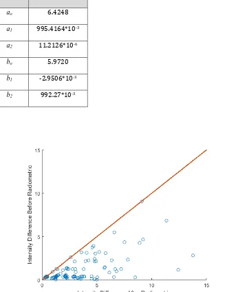
Second, the radiometric similarity is utilize for the best verification. Sometimes, geometric distortion by relief and different orientation of images may affect the match result. For best radiometric similarity a comparison with the shift value of key points have been utilized. It is restricted by small area around key points in both images called search area. Sum of absolute difference (SAD) of radiometric similarity is checked for best correspondence between these points which is [23]:.
(
,
)
(
',
')
2 1
x
y
I
x
y
I
SAD
…. (26)Where I1(x,y) and I2(x’,y’) are the intensity of the reference and sensed image respectively. A window
of (3*3), (5*5), or (7*7) are check as sequences if not found in one of them the following one is tested.
4. RESULT AND DISCUSSIONS
A computer simulation was applied in this work for image of Mars ((data set name:” MARS
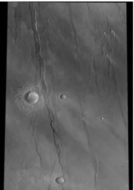
EXPRESS HRSC MAP PROJECTED REFDR V3.0”, product creation time:” 2016-03-02T11:36:00.000Z”). The image of Mars is shown
[image:6.612.357.489.291.479.2]in figure (3).
Figure 3. Mars Express Hrsc Map Projected Refdr V3.0.
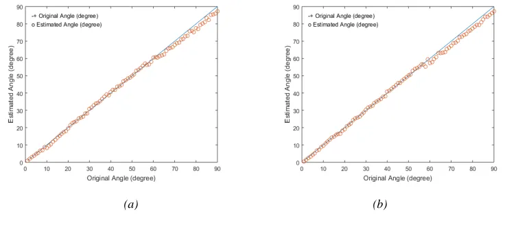
4.2.Scaling Result
[image:7.612.92.516.67.260.2]
(a) (b)
Figure 4. Estimation Of: (A) Scale Value. (B) Its Percentage Error.
The aim of this step is to estimate the scale value between two image of the same scene (the reference and the sensed one). The result is showning in figure (4a) between the real value and the estimated one. The error percentage in figure (4b) reveal its deviation from the real value. The estimation of scale value is reveal a good estimation especially when the scale value larger than one becaue of increase its resolution and size of its feature as compared when its below one. Features of image of planet has low in contrast and number features and have a best estimate when it is large the original one. The erosion of the surface of planet may affect on its number and distinguish its features.
4.1. Rotation Result
The result of using methods for rotation estimation value for image contaminate with rotation and scale effect.
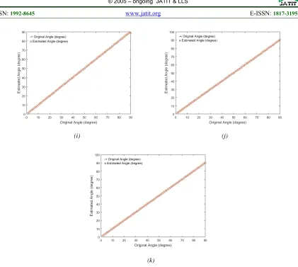
The estimation rotation was applied on an sensed image which has scale values (0.5-1.5) of the reference image. Ecah value of scale, which is (0.1), a rotation estimation is evaluated for values ( 1o90o) as in the following figures.
[image:7.612.127.495.518.682.2]
(c) (d)
(e) (f)
(i) (j)
[image:9.612.100.521.59.436.2](k)
Figure 5. Rotation Estimation Value To Angle (1o90o) With Scale Value: (A) 0.5, (B) 0.6 (C) 0.7, (D) 0.8, (E) 0.9, (F) 1, (G) 1.1, (H) 1.2, (I) 1.3, (J) 1.4, (K) 1.5.
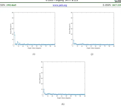
The error percentage for the rotation value for each sitution is showining below:
(c) (d)
(e) (f)
(i) (j)
[image:11.612.92.517.60.436.2](k)
Figure 6. Error Percentage For Rotation Estimation Value For Angle (1o90o) When Scale Value: (A) 0.5, (B) 0.6, (C) 0.7, (D) 0.8, (E) 0.9, (F) 1, (G) 1.1, (H) 1.2, (I) 1.3, (J) 1.4, (K) 1.5.
From the figure (5) reveal that method for estimating rotation value show a good estimation when there is a variation in its scale (0.5-1.5). The
small range of scale value represent the maximum range of variation of altiude of satellite that occure. The variation of altitude may be refer to the path of satelite or to unstabilities of its sensor or the effect of matual influnce of gravity that affect on it. The reboost of this estimateion can show in percent error in figure (6). When the scale value is less than one it reveals a small variation in finding its rotation value this is due to low resolution that affect on its feature. Instead of that, when the resolution value is large than one, show a good estimation of rotation value. For the value of scale (1) the variation in its result because of the compution of scale method which depends on the
bicubic interpolation which affect its intensity values.
4.2. Match Result
Table.(1): parameter values of affine transform
Coefficient value
ao 6.4248
a1 995.4164*10-3
a2 11.2126*10-6
bo 5.9720
b1 -2.9506*10-3
[image:12.612.138.465.125.549.2]b2 992.27*10-3
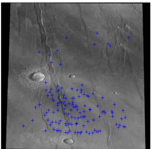
[image:12.612.177.445.329.556.2]Figure 8. Key Points Of The Reference Image (Mars Image).
Find match between two images means find its correspond one by identify match control points. In this work a new proposed method for locate these points was established. The match points are computed by applying equation (22) and (23). The two criteria that are used for match which is distance and angle. These two criteria are related on each other. For example, if any point can have similar angle with unequal distance consider an outlier according to equation (22) and vice versa. The number of key points (sift-points) that are found in the reference image are (3139) point with (3230) point for the sensed one. The difference in their number because the sensed one is the best repaired one from geometric distortion (scale and rotation). The final number of the match between them after the verification are (126) point as shown in figure (8) and (9). For the verification a spatial registration with its radiometric similarity are utilized. Table (1) represent the values of the parameter of equation (24) and (25) which evaluated from sift-points. Sometimes, geometric distortion by relief and different orientation of images may affect the match result. For best radiometric similarity a comparison with the shift value of key points have been utilized with equation (26). The result can show in scatter plot in figure (7). The scatter plot reveal that the diagonal line represents unaffected points. The shifted points to the correct position is on the horizontal axis while the vertical axis represent the inverse of that.
5. CONCLUSIONS
The preprocessing steps for estimating rotation and scaling value made match more accurate. This step is necessary on the quality of selection of accurate points especially with these images. The selection of range of scale values with rotation relate to the range of geometric distortion that represent paths of satellite with its attributes. The new algorithm for estimation of scale valve with range (0.5-1.5) associated with rotation angle
(1o90o) shows good estimation for them. The
auto detection method shows a good match as shown in result. The proposed method for matching which relay on the distance and angle with its
good match points. This procedure may extend to include multispectral images of planets and image of our life.
5. COMPARISONS WITH PREVIOUS
STUDIES:
Many methods have been developed for the automatic image matching for the different line of life. These methods were used a spatial domain and others depend on the frequency domain. The proposed method for this paper is state on the spatial domain with the geometrical relationship with its neighbors. As compared with other methods it uses the relation of distance and angle for image of planet which has features and contrast as compared to others.
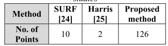
The following table is show the comparison of the proposed method with two methods on the same data set with the similar condition. The first one is SURF (Speed up Robust Features) detector. The difference is in the number of the matched points in both images.
Table (2): Comparing the match points previous studies
Method SURF [24] Harris [25] Proposed method No. of
Points 10 2 126
REFERENCES
[1] T. Lindeberg, "Feature detection with automatic scale selection," International journal of computer vision, vol. 30, pp.
79-116, 1998.
[2] U. Jayaraman, A. K. Gupta, S. Prakash, and P. Gupta, "An enhanced geometric hashing," in Communications (ICC), 2011 IEEE International Conference on, 2011,
pp. 1-5.
[3] F. Tombari and L. Di Stefano, "Improving Geometric Hashing by Means of Feature Descriptors," in VISAPP, 2011, pp.
419-425.
[image:14.612.330.503.389.437.2][5] J. Wu, Z. Cui, V. S. Sheng, P. Zhao, D. Su, and S. Gong, "A Comparative Study of SIFT and its Variants," Measurement Science Review, vol. 13, pp. 122-131,
2013.
[6] K. A. Sallal and A.-M. S. Rahma, "Invariants Feature Points Detection based on Random Sample Estimation,"
International Journal of Computer Applications, vol. 86, 2014.
[7] Y. Yu, K. Huang, and T. Tan, "A Harris-like scale invariant feature detector," in
Asian Conference on Computer Vision,
2009, pp. 586-595.
[8] K. Mikolajczyk and C. Schmid, "An affine invariant interest point detector," in
European conference on computer vision,
2002, pp. 128-142.
[9] D. G. Lowe, "Distinctive image features from scale-invariant keypoints,"
International journal of computer vision,
vol. 60, pp. 91-110, 2004.
[10] K. Mikolajczyk and C. Schmid, "Scale & affine invariant interest point detectors,"
International journal of computer vision,
vol. 60, pp. 63-86, 2004.
[11] D. G. Low, "Object recognition from local scale-invariant features," in Proceedings of the International Conference on Computer Vision, 1999, pp. 1150-1157.
[12] P. Panchal, S. Panchal, and S. Shah, "A comparison of SIFT and SURF,"
International Journal of Innovative Research in Computer and Communication Engineering, vol. 1, pp.
323-327, 2013.
[13] W. Sze, W. Tang, and Y. Hung, "Singular-value-decomposition based scale invariant image matching," in Vision Geometry XIV,
2006, p. 60660I.
[14] E. Delponte, F. Isgrò, F. Odone, and A. Verri, "SVD-matching using SIFT features," Graphical models, vol. 68, pp.
415-431, 2006.
[15] G. L. Scott and H. C. Longuet-Higgins, "An algorithm for associating the features of two images," in Proc. R. Soc. Lond. B,
1991, pp. 21-26.
[16] H. Wu, M. J. Hayes, A. Weiss, and Q. Hu, "An evaluation of the Standardized Precipitation Index, the China-Z Index and the statistical Z-Score," International journal of climatology, vol. 21, pp.
745-758, 2001.
[17] A. A. Goshtasby, Image registration: Principles, tools and methods: Springer
Science & Business Media, 2012.
[18] N. Mat-Isa, M. Mashor, and N. Othman, "Seeded region growing features extraction algorithm; its potential use in improving screening for cervical cancer,"
International Journal of The Computer, the Internet and Management, vol. 13, pp.
61-70, 2005.
[19] S.-H. Chang, F.-H. Cheng, W.-H. Hsu, and G.-Z. Wu, "Fast algorithm for point pattern matching: invariant to translations, rotations and scale changes," Pattern recognition, vol. 30, pp. 311-320, 1997.
[20] S. H. AL-KILIDAR and L. E. GEORGE, "TEXTURE RECOGNITION USING
CO-OCCURRENCE MATRIX
FEATURES AND NEURAL
NETWORK," Journal of Theoretical & Applied Information Technology, vol. 95,
2017.
[21] M. G. Madden, Ó. Brádaigh, and M. Conchúr, "NUI Galway-UL Alliance Engineering, Informatics and Science Research Day 2013-Book of Abstracts," ed: NUI Galway, 2013.
[22] S. Liang, X. Li, and J. Wang, Advanced remote sensing: terrestrial information extraction and applications: Academic
Press, 2012.
[23] R. A. J. Mohammed, F. M. Abed, and L. E. George, "Improved Automatic Registration Adjustment of Multi-source Remote Sensing Datasets," Journal of Engineering, vol. 21, pp. 61-81, 2015.
[24] H. Bay, A. Ess, T. Tuytelaars, and L. Van Gool, "Speeded-up robust features (SURF)," Computer vision and image understanding, vol. 110, pp. 346-359,
2008.
![Figure 2. Seed Filling tech [18].](https://thumb-us.123doks.com/thumbv2/123dok_us/8900360.954654/4.612.322.487.262.421/figure-seed-filling-tech.webp)