Date of publication xxxx 00, 0000, date of current version xxxx 00, 0000. Digital Object Identifier 10.1109/ACCESS.2017.Doi Number
Color Constancy Algorithm for Mixed-illuminant
Scene Images
M. A. Hussain and, A. Sheikh Akbari
School of Computing, Creative Technology and Engineering, Leeds Beckett University, Leeds, UK. Corresponding author: A. Sheikh Akbari (e-mail: [email protected]).
ABSTRACT The intrinsic properties of the ambient illuminant significantly alter the true colors of objects within an image. Most existing color constancy algorithms assume a uniformly lit scene across the image. The performance of these algorithms deteriorates considerably in the presence of mixed illuminants. Hence, a potential solution to this problem is the consideration of a combination of image regional color constancy weighing factors (CCWFs) in determining the CCWF for each pixel. This paper presents a color constancy algorithm for mixed-illuminant scene images. The proposed algorithm splits the input image into multiple segments and uses the normalized average absolute difference (NAAD) of each segment as a measure for determining whether the segment’s pixels contain reliable color constancy information. The Max-RGB principle is then used to calculate the initial weighting factors for each selected segment. The CCWF for each image pixel is then calculated by combining the weighting factors of the selected segments, which are adjusted by the normalized Euclidian distances of the pixel from the centers of the selected segments. Experimental results on images from five benchmark datasets show that the proposed algorithm subjectively outperforms the state-of-the-art techniques, while its objective performance is comparable to those of the state-of-the-art techniques.
INDEX TERMS color constancy, multiple illuminants, segmentation, Max-RGB.
I. INTRODUCTION
Human eyes are analogous to the source illuminant and can see the true colors of objects, whereas digital images are often influenced by the color of the prevailing illuminant, the intrinsic reflectance properties of the objects, and the sensitivity functions of the capturing devices [1-3]. These factors cause the captured images to exhibit color casts, rather than presenting the actual colors of the objects [4-5]. The goal of a color constancy algorithm is to remove the color casts from the image to manifest the actual colors of the objects by maintaining a constant distribution of the light spectrum across the digital image so that the image appears as if it has been taken under a canonical source illuminant [6-7]. Over the years, a considerable number of color constancy algorithms have been reported in the literature [8-45]. These algorithms can be categorized as statistical, gamut-based, physics-based, and illuminant-parameter-based approaches.
Statistical approaches exploit the color information of the image to estimate the scene’s illuminant. The Gray World and White Patch techniques are the two classic algorithms of
this group. The Gray World method assumes that the average values of the three image color components are achromatic and representative of their gray levels [8]. The White Patch method assumes that the maximum values of the image color components are equal; it is also known as the Max-RGB algorithm [9]. Finlayson and Trezzi [10] proposed the Shades of Gray algorithm for reducing the data dependency of the Gray World and White Patch algorithms by using the Minkowski norm (p=6) as a mathematically rigorous tool. Gisenji et al. [11] put forward the Gray Edge hypothesis algorithm. This technique assumes that the absolute values of the image derivative (edge) color components are achromatic. This algorithm was further extended by considering various edge types; the extended algorithm is known as the Weighted Gray Edge method [12].
The gamut-based color constancy algorithm was introduced by Forsyth [13]. This technique assumes that only a limited number of colors can be observed for a given illuminant in the image of a real-world scene. Finlayson [14] used the chromaticity space to compute the gamut, which
2 VOLUME XX, 2017 reduces the influence of many restrictions of Forsyth’s
algorithm [13]. Finlayson and Hordley [15] achieved further improvement of Finlayson’s method [14] by using a 3D approach to generate a more coherent map from the feasible Gamut sets.
Physics-based methods exploit the information of the reflective interaction between the object and the illuminant. These methods assume that all pixels of a surface belong to a plane in the RGB space and the intersections of these surfaces are used to estimate the color of the source illuminant. Several physics-based methods have been reported in the literature [16-19]. Computation of the scene illuminant using specular highlights was proposed in [16]. This method was further extended in [17], where a standard surface-reflection model is used to estimate the source illuminant without using the reference white standard. Gerald et al. [18] used correlation of physical and statistical color information of the surface light to estimate the scene illuminant. Liao et al. [19] proposed a color constancy algorithm based on the photographic technique that is used to determine optimal film exposure and negative film development. In this algorithm, the total tonal value of the image histogram is divided into 11 sections, which range from 0 to 10 as pure black to pure white, respectively. Empirically, they noticed that 18% of the reflectance values are in the middle gray zone (zone 5) on a geometric scale from black to white. Hence, the researchers used 𝑌𝐶𝑏𝐶𝑟 color
space to detect the color cast on the middle gray level and then adjusted the image to match the zones with their respective brightnesses.
The methods that are described above are based upon the notion that the illuminant is uniform across the scene. However, in practice, real-world scenes are usually lit by multiple illuminants, which results in these techniques not being able to handle the color constancy of the images properly. Hence, multiple illuminant color constancy methods have been considered by researchers [20-42]. A considerable number of these techniques propose that light estimation must be performed locally by assuming that a small area of the image is illuminated by a uniform light source and employ different segmentation and fusion strategy for image adjustment [20-25].
Xu et al. proposed a global-based video enhancement in [20]. Their proposed technique analyses the features of different Region of Interests (ROIs). It then applies two fusion strategies, namely: piecewise-based and factor-based fusions, to create a global tone mapping curve for the whole image. They have reported superior perceptual quality to those considered state of the art. Chen et al. proposed an intra-and-inter-constraint-based algorithm for video enhancement. Their proposed algorithm applies AdaBoost-based object detection on the input video frames to obtain Region Of Interests (ROIs). The proposed method uses mean and standard deviation of each ROI to analyze features of different ROIs. After extracting and analyzing the features
from different ROIs, a global piecewise tone mapping curve for the entire frame is created by fusing the features of different ROIs such that different regions inside a frame can be suitably enhanced at the same time [21]. Riess et al. [22] reported a color constancy method for real-world mixed-illuminant scene images, which estimates the local illuminant for distinct mini image regions using a graph-based algorithm. Their algorithm performed comparably against the state-of-the-art methods on single-illuminant images. However, the effectiveness of their algorithm on real-world images was insufficient. Gisenji et al. proposed a multi-illuminant color constancy algorithm in [23]. The proposed method uses a sampling method, such as: grid-based, keypoint-based or segmentation-based sampling method, to sample P patches from the image. It is assumed that the color of the light source is uniform over each patch and the union of all patches covers the entire image. The proposed technique then applies one of the traditional color constancy methods on every patch to estimate their local illuminants. To reduce the illuminant estimation error, patches illuminated by the same light source taken from different parts of the image are combined to form a large patch. After different estimates are grouped together into N groups, the result is back-projected onto the original image, generating pixel-wise illuminant estimation. The proposed algorithm then uses the Von-Kries model to perform color constancy adjustment for every pixel of the image. Addressing the problem of inherent estimation of the local illuminant in [23], a method that considers not only the illuminant colors but also the spatial distribution of the illuminant colors using a conditional random field was proposed in [24]. This technique employs an energy minimization framework of the spatial distribution and a combination of several statistical and physics-based methods into a single multi-illuminant estimation task. The researchers reported significant objective results on multi-illuminant images. A super-pixel-based multi-multi-illuminant color constancy algorithm was reported in [25]. This algorithm applies Veksler et al.’s [26] segmentation algorithm to segment the input image into a set of super-pixels such that all super-pixels in a single super-pixel have the same color value. The underlying assumption is that the illumination is approximately constant on a single super-pixel. It then applies Gray World, 1st order Gray Edge, 2nd order Gray Edge, Bayesian and Gamut mapping 2D &3D color constancy algorithms on each super-pixel independently. The performance of the algorithm for using three different fusion methods, namely: average of all combined estimates, Gradient tree boosting and Random forest regression, on a set of images were evaluated. They reported that their corrected images, using the combined estimate methods, exhibit higher errors compared to using the uniform estimates. They concluded that the combinations of single-illuminant estimators yield promising results to address the recovery of illuminant color under non-uniform
illuminants.
To account for illumination variations in the scene, several learning-based algorithms have been proposed in the literature [27-29]. Baron [27] formulated the color constancy problem as a 2D spatial localization task in a log-chrominance space. He noticed that scaling the image color channels induces a translation in the log-chromaticity histogram, which enables the color constancy problem to be approached using tools such as convolutional neural network (CNN). An illuminant estimation method that uses a convolutional neural network that consists of one convolutional layer, one fully connected neural network layer and three output nodes was proposed by Bianco et al.
[28]. This CNN based method samples multiple non-overlapping patches from the input image and then applies a histogram stretching technique to neutralize the contrast of the image. The algorithm then combines the patch scores, which are obtained by extracting activation values of the last hidden layer to estimate the illuminant. The researchers reported satisfactory performance of the algorithm on a specific raw image dataset. However, they did not report any experimental results on benchmark image datasets. Fourure
et al. [29] proposed an extension of the neural-network-based method by using a mix-pooling approach that determines the availability of accurate features to be learned for the color constancy algorithm without relying on unitary or handcrafted approaches. This algorithm uses a neural network that is based on Minkowski pooling and a fully connected layer to learn a suitable deep model.
Instead of explicitly estimating the scene illuminant, alternative biologically inspired models for color constancy were proposed in [30-32]. Gao et al. [30] imitated the response of the double-opponent cells in separate channels and estimated the illuminant color by the 𝑚𝑎𝑥- or 𝑠𝑢𝑚 -pooling mechanism in long, medium and short wavelength color space. The mechanism of the horizontal cell (HC) modulation, which provide a global color correction, was embedded into the neural-network-based model in [31]. The model that was proposed in [32] is based on the functioning of the human brain, which relies largely on the local contrast to preserve the actual object color.
Other multiple-illuminant algorithms are based on the detection of particular pixels for color correction. Jaehyun et al. [33] reported an approach of detecting a saturation-free, pure white point using a dark-channel prior. Yang et al. [34] proposed an efficient gray pixel detection method, which is used for source illuminant estimation, even for image regions with a very low presence of gray pixels, with an illuminant-invariant measure. Mazin et al. [35] introduced the concept of the Planckian Locus, which refers to the color of a black body whose temperature changes are defined by the chromaticity space. Pixel sets that are closer to the Planckian Locus are considered more reliable by the authors for illuminant estimation. Bianco and Schettini [36] exploits the pixels around face regions for color constancy by using a
scale-space histogram filtering method. In [37], the authors applied hard and soft segmentation approaches to generate a rough 3D geometric model to relate the statistical information of its layers to a suitable color constancy method. Joze and Drew [38] used texture features and weakly color constant RGB values to find the neighboring surface from the training data; the surface is an estimate of the local light source. An alternative approach was proposed in [39], where lattices of different scales of image were used to estimate the illuminant. Finlayson [40] introduced a moment-based algorithm that uses several higher-order moments of the color features on a fixed 3×3 matrix transformation. Cheng et al. [41] proposed a color constancy algorithm that uses a diagonal 3×3 matrix based on the ground-truth illumination of a 24-color patch. This algorithm outperforms the traditional diagonal correction methods. However, the application of this method is limited to images with color patches, so benchmark datasets without color patches are ignored. Cheng et al. [42] proposed an algorithm for estimating two illuminants using the large sub-regions of an image. In this algorithm, a single-illuminant estimation method is used on large image regions to determine several illumination estimation candidates for the scene. The user preference is then used to select the best-performing illuminants manually and subjectively. Many of the aforementioned multi-illuminant color constancy algorithms assume that the scene is illuminated by one or two light sources. Despite their effectiveness with two illuminants, in practice, these algorithms may not be able to tackle scenes that are lit by more than two illuminants. Moreover, the local estimation and combination through various sampling processes of some of these algorithms are too sophisticated and require complex reasoning. We have shown in [43-45] that circumventing large uniform color patches could improve the performance of the statistics-based methods when dealing with single-illuminant images.
Investigating this concept much more meticulously, this paper presents a color constancy algorithm for multiple- illuminant images by combining the initial color constancy weighing factors of the image segments using a Euclidian distance regulating factor for each pixel. The proposed algorithm divides the input image into multiple segments based on their color features, using the K-means++ clustering method. Each segment’s color variability is assessed using the normalized average absolute difference (NAAD) of its color components. Segments with NAAD values that are greater than the empirically determined threshold values are chosen for color constancy adjustment. The Max-RGB method is then applied to the selected segment to calculate its local weighting factors. The weighing factor for each pixel is then calculated by fusing the weighting factors of the selected segments, which are weighted by the normalized Euclidian distances of the pixel from the centers of the selected segments. Experimental results on five benchmark single- and multiple-illuminant image datasets confirm that
4 VOLUME XX, 2017 the proposed method significantly outperforms the
state-of-the-art algorithms. The rest of the paper is organized as follows: Section 2 describes the proposed algorithm, Section 3 presents experimental results, and Section 4 presents the conclusions of the paper.
II. COLOR CONSTANCY ALGORITHM FOR MIXED-ILLUMINANT SCENE IMAGES
The proposed color constancy adjustment algorithm for a multi-illuminant scene image can be divided into the three steps:
1. Image segmentation based on its color features; 2. Color variability assessment and local weighting
factor calculation using the Max-RGB algorithm; 3. Calculation of color constancy weighting factors
for each pixel by combining the weighting factors of the selected segments.
2.1 IMAGE SEGMENTATION
The proposed algorithm splits the input image into multiple segments using the K-means++ method [46], although any other segmentation method can be used. Experiments on various images showed that the proposed algorithm performs well with a minimum of four segments. To facilitate color-difference-based segmentation, it converts the input image into the L*a*b* color space, where the a* and b* components contain the color information of the image. The centroid selection and segmentation steps of the K-means++ algorithm are as follows:
i. Select four initial centroids Ci in the a*b* color space randomly, where i = 1, 2, ...,4.
ii. Calculate the Euclidian distance from each component to Ci.
iii. Assign each component to its closet centroid based on that distance.
iv. Re-calculate the average of the initial segments to obtain a new centroid location.
v. Re-calculate the Euclidian distance from each point to the new centroid and assign each component to its nearest centroid.
vi. If no component is re-assigned, then these are the final segments; else, return to step ii.
2.2 COLOR VARIABILITY ASSESSMENT AND LOCAL WEIGHTING FACTOR CALCULATION USING THE MAX-RGB ALGORITHM
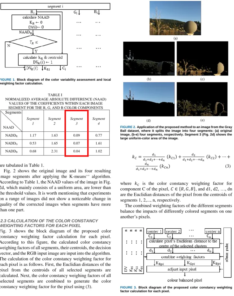
Fig. 1 shows the block diagram of the color variability assessment of the image segments and the local weighting factor calculation using the Max-RGB algorithm. The proposed technique calculates the normalized average absolute difference (NAAD) for the R, G and B components of the input image segments individually using (1).
𝑁𝐴𝐴𝐷𝐶𝑠 = 1
𝑁×𝑠̅𝐶∑ ∑|𝑃𝐶− 𝑆̅𝐶| (1)
where C represents the segment color component, 𝐶 ∈ {𝑅, 𝐺, 𝐵}; 𝑁𝐴𝐴𝐷𝐶𝑆 is the NAAD value of component C of
segment S, 𝑃𝐶 is component C of the pixel and 𝑆̅𝐶 is the
average value of component C of the segment; N is the total number of pixels of the segment; and | | is the absolute value operator.
The Average Absolute Difference (AAD) is a measure to quantify the color uniformity of the segment’s pixels. Since uniform color patches could potentially bias the color constancy adjustment factors towards the color of the big uniform areas, the AAD criterion was normalized to make it independent of the number of pixels within the segment. This permits generalized AAD across images with different sizes and number of segments.
The resulting NAAD values of the segment are then compared with the three empirical threshold values, which are denoted as TR, TG and TB, in the block diagram for the R,
G and B components, respectively. If the NAAD values are greater than the thresholds, it is assumed that the segment has sufficient color variation to contribute to the whole image color constancy adjustment; hence, it will be chosen and a bit in the decision vector (DV) that represents this segment will be set. The centroid of the segment (Ci for segment i in the block diagram) and the Max-RGB-based color constancy weighting factors for this segment, which are denoted as KR, KG and KB, respectively, are calculated. KR, KG and KB are calculated using (2).
𝐾𝐶 =𝑠̅𝑚𝑎𝑥 ∑ 𝑃𝑐𝑚𝑎𝑥
𝑁
⁄ (2)
where 𝐾𝐶 is the weighting factor of component C (𝐶 ∈
{𝑅, 𝐺, 𝐵} ), 𝑠̅𝑚𝑎𝑥 is the average value of the segment’s
column’s maximum values for the R, G and B components,
∑ 𝑃𝑐𝑚𝑎𝑥 is the sum of the maximum values of the
components of segment C, and N is the total number of pixels in the segment.
In this paper, the Max-RGB color constancy method was used to calculate the initial segment’s color constancy adjustment factors. Although any other statistical color constancy method such as Gray World [8], Shades of Gray [10], Gray Edge (1-2) [11], Weighted Gray Edge [12], and Gray Pixel [34], can be used. However, the reason for using the Max-RGB method in this research is that the Max-RGB method is computationally less intense.As a pre-processing step, extensive experiments were performed using the benchmark image dataset to determine the number of segments and the threshold values. The results showed that a threshold value of 0.01 for the TR, TG and TB components and the selection of four segments can efficiently eliminate segments with uniform areas. The influence of different number of segments on the performance of the proposed method is shown in Table 5. To gain insight into the NAAD values of different image segments, the calculated NAAD values for a sample image from the Gray Ball dataset [47]
FIGURE 1.Block diagram of the color variability assessment and local weighting factor calculation.
TABLE I
NORMALIZED AVERAGE ABSOLUTE DIFFERENCE (NAAD) VALUES OF THE COEFFICIENTS WITHIN EACH IMAGE SEGMENT FOR THE R, G, AND B COLOR COMPONENTS
NAAD Segment 1 Segment 2 Segment 3 Segment 4 NADDR 1.17 1.63 0.09 0.77 NADDG 0.53 1.65 0.07 1.61 NADDB 0.68 2.31 0.04 1.02
are tabulated in Table 1.
Fig. 2 shows the original image and its four resulting image segments after applying the K-means++ algorithm. According to Table 1, the NAAD values of the image in Fig. 2d, which mainly consists of a uniform area, are lower than the threshold values. It is worth mentioning that experiments on a range of images did not show a noticeable change in quality of the corrected images when segments have more than one part.
2.3CALCULATION OF THE COLOR CONSTANCY
WEIGHTING FACTORS FOR EACH PIXEL
Fig. 3 shows the block diagram of the proposed color constancy weighting factor calculation for each pixel. According to this figure, the calculated color constancy weighing factors of all segments, their centroids, the decision vector, and the RGB input image are input into the algorithm. The calculation of the color constancy weighting factor for each pixel is as follows. First, the Euclidian distances of the pixel from the centroids of all selected segments are calculated. Next, the color constancy weighing factors of all selected segments are combined to generate the color constancy weighting factor for the pixel using (3).
FIGURE 2. Application of the proposed method to an image from the Gray
Ball dataset, where it splits the image into four segments: (a) original image, (b-e) four segments, respectively. Segment 3 (Fig. 2d) shows the large uniform-color area of the image.
𝑘𝐶= 𝑑1 𝑑1+𝑑2+⋯+𝑑𝑛 (𝑘𝐶1) + 𝑑2 𝑑1+𝑑2+⋯+𝑑𝑛 (𝑘𝐶2) + ⋯ + 𝑑𝑛 𝑑1+𝑑2+⋯+𝑑𝑛 (𝑘𝐶𝑛) (3)
where 𝑘𝐶 is the color constancy weighting factor for
component C of the pixel, 𝐶 ∈ {𝑅, 𝐺, 𝐵}, and d1, d2, …, dn are the Euclidian distances of the pixel from the centroids of segments 1, 2,..., n, respectively.
The combined weighting factors of the different segments balance the impacts of differently colored segments on one another’s pixels.
FIGURE 3. Block diagram of the proposed color constancy weighting factor calculation for each pixel.
6 VOLUME XX, 2017 III. EXPERIMENTAL RESULTS
To generate experimental results and compare the performance of the proposed color constancy adjustment technique with those of state-of-the-art techniques, five benchmark multiple- and single-illuminant image datasets were selected. The proposed and the state-of-the-art algorithms were applied to the images of these datasets. The resulting images were then subjectively and objectively assessed. The results show the merits of the proposed technique over the state-of-the-art algorithms. In sub-section A, the five datasets are introduced. Performance measurement criteria are given in sub-section B and experimental results are presented in sub-section C.
A. IMAGE DATASETS
1) MULTIPLE-LIGHT-SOURCE (MLS) DATASET [23] The dataset contains 58 indoor images that were captured under different illumination conditions and 9 low-resolution outdoor images of various sizes with two distinct illuminants. The ground truths of these outdoor images were computed by placing and manually annotating several gray balls in the scene.
2) MULTIPLE ILLUMINANT AND MULTIPLE OBJECT (MIMO) DATASET [24]
The dataset is comprised of 58 laboratory images that were taken indoors under controlled lighting conditions and 20 real-world images that were taken under uncontrolled lighting conditions.
3) GRAY BALL DATASET [47]
This dataset consists of a total of 11,340 images of size 240×360 from a range of scenarios, which were taken under natural single- or mixed-illuminant lighting conditions, where a gray-ball was placed in front of the video camera. Consequently, there are many images of nearly identical scenes. Two hundred images from this dataset, which cover a good range of scenes and lighting conditions, were chosen to generate experimental results.
4) GEHLER AND SHI DATASET [48]
The Gehler and Shi dataset contains 568 images of people, places and various objects from indoor and outdoor scenes, where a Macbeth color checker chart is placed in a known location of every scene. This dataset covers both single- and multiple-illuminant natural images and among them, one hundred images were used for subjective evaluation.
5) RAISE DATASET [49]
This dataset contains 8156 high-resolution, raw, challenging images from real-world scenes. They were primarily designed for evaluating the performance of image forgery algorithms and for other fields of research that deal with image analysis, processing and understanding. From this dataset, 250 images, which cover both indoor and outdoor scenes that are illuminated by either a single or multiple
illuminants, were chosen to generate experimental results.
B. PERFORMANCE MEASUREMENT CRITERIA
The color constancy performance measurement criteria are divided into two main categories: objective and subjective measures. In objective assessment, color constancy performance is evaluated by comparing the resulting image with its ground truth. Euclidian distance and angular error are the two most commonly used distances measures for measuring the objective quality of the color-balanced images, of which the angular error is widely used in the literature. The angular error of a color-balanced image is determined by calculating the angular distance of that image from its ground truth using (4).
𝑎𝑛𝑔𝑢𝑙𝑎𝑟 𝑒𝑟𝑟𝑜𝑟 = cos−1(𝐼̂
𝐺. 𝐼̂𝐶𝐶 ) (4)
where 𝐼̂𝐺 and 𝐼̂𝐶𝐶 denote the normalized ground-truth and the
normalized color constancy image illuminant vectors, respectively.
In general, the average of the mean and the median of the angular error over many images is used to evaluate the performance of a color constancy algorithm. The summary statistics of the Angular Error indicate that the algorithm with the lower mean or median has better performance. However, there is substantial debate about the correlation between the objective results and human perception. In Section 3.1, the contradictions between subjective and objective results are discussed in detail. This paper uses subjective evaluation as the key measure for assessing the quality of the images, since human perception is the key measure for evaluating the color constancy of the images.
Therefore, some samples of the corrected images by the proposed and state-of-the-art techniques are illustrated in the results section to enable the reader to assess and compare achieved visual qualities across different techniques. In addition, a Mean Opinion Score (MOS) assessment on a selection of images from different datasets was conducted to give a quantitative sense on the achieved subjective qualities. C. RESULTS AND EVALUATION
Experimental results were generated by applying the proposed technique with state-of-the-art and other existing color constancy algorithms, namely Max-RGB (White Patch) [9], Shades of Gray [10], Gray Edge (1-2) [11], Weighted Gray Edge [12], the method of Gisenji et al. [23], MIRF [24], CNN [28], Gray Pixel [34], Exemplar method [38], and the method of Cheng et al. [42], to the images of the five aforementioned image datasets.
The results show that the proposed technique’s images exhibit the highest subjective color constancy and the best objective qualities across almost every summary statistic. In the following, examples of achieved subjective and objective color constancy are given to enable the reader to compare the proposed technique with the state-of - the-art and other
existing techniques.
To demonstrate the achieved subjective color constancy, 4 sample images from the MIMO dataset, two images from the Gehler and Shi Dataset, one sample image from the Gray Ball dataset, and 3 images from the RAISE dataset, which cover a variety of sceneries and include natural- and laboratory-setting objects that are illuminated by one or more illuminants, were chosen and color balanced using the proposed, state-of-the-art and other existing techniques. The resulting images are shown in Fig. 4-8.
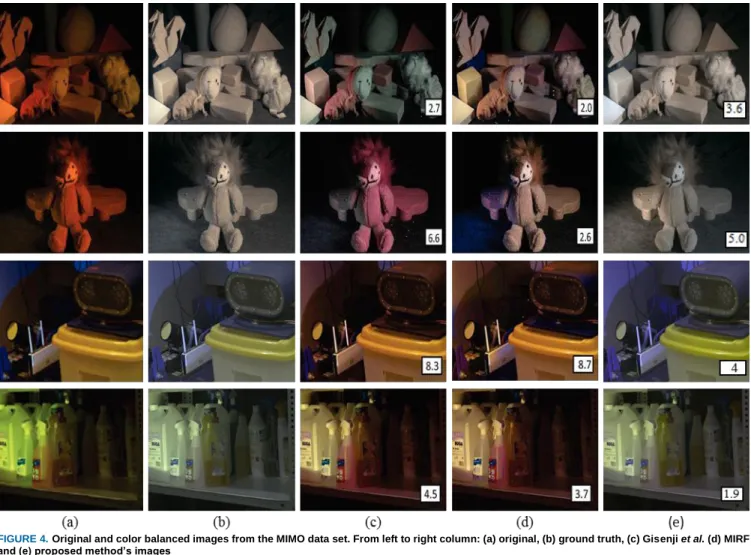
Fig. 4 shows four original sample images from the MIMO dataset and corresponding color-balanced images that were obtained using the proposed technique and two state-of-the-art techniques, namely the method of Gisenji et al. [23] and MIRF [24]. The input images are shown in column ‘a’ of Fig. 4 and are named ‘toys’, ‘lion’, ‘camera’ and ‘detergents’ from top to bottom, respectively. The corresponding ground truths of the input images and the images that were obtained by the method of Gisenji et al., MIRF and the proposed method are shown in columns b to e, respectively. The original images and those that were obtained by MIRF and the method of Gisneji et al. are directly taken from [24]. According to the images that were obtained by Gisenji et al.’s method (column c), a) the source illuminant colors of
the ‘toys’ and the ‘lion’ are not completely removed; b) the ‘lion’ image color is biased to red and c) the ‘toy’ image suffers from severe blue saturation. According to the images that were obtained by the MIRF method (column d), a) MIRF images exhibit higher color constancy than Gisenji et al.’s
images, b) MIRF’s images show some erroneous color correction, e.g., extreme purple color in the bottom-left part of the ‘lion’ image; and c) the colors of the ‘toys’ and the ‘detergents’ images do not look original, as yellow illuminant is still obvious on the objects. According to the proposed method’s images (column e), a) the ‘toys’, ‘lion’ and ‘detergents’ images exhibit the highest color constancy and, although the ‘cameras’ image still shows some bluish color cast, in comparison to the images of Gisenji et al. and MIRF, it still has the highest color constancy. The angular errors of the resulting images are also shown on the images. By comparing the perceptual quality of the images and their angular errors, we observe that a) although the ‘toys’ and ‘lion’ images of the proposed method look very natural and have the highest color constancies compared to the images of Gisenji et al. and MIRF, their angular errors are higher than those of the images of Gisenji et al. and MIRF. This supports the argument that objective measures are not always consistent with the achieved subjective qualities.
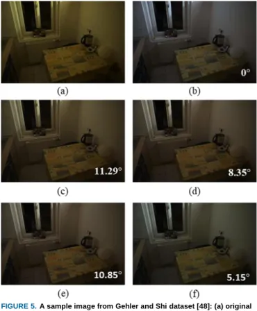
Fig. 5 shows a sample image from the Gehler and Shi dataset, its ground truth and its color-balanced images that were obtained using Gray Edge-1, Weighted Gray Edge (WGE), Convolutional Neural Network (CNN) and the proposed method. The mean angular errors of the color balance images are also calculated and specified in the lower-right corner of each image. From Fig. 5a, the original
image appears to be illuminated by a warm yellow light, where the white background, the table cloth and the white ball on the table all are color casted by the yellow illuminant. Fig. 5b shows the ground-truth image, as it would appear if taken under canonical light. Fig. 5c shows the Gray Edge-1 method’s image. This image exhibits a greatly reduced yellow color cast. However, the color cast of the image on the wall in the background is noticeable. Fig. 5d shows WGE’s image. Although WGE’s image exhibits higher color constancy in comparison to the Gray Edge-1 method’s image, the effect of the illuminant on the wall in the background and on the table cloth is obvious. The CNN (fine-tuned) method’s image (shown in Fig. 5e) shows an infinitesimal improvement in the table cloth illuminant over WGE’s image. However, the illuminant color difference on the background wall between this image and the ground-truth image is evident. The proposed method’s image is shown in Fig. 5f. This image is almost the same as the ground-truth image. By comparing the angular error of the images, we determine that the angular error of the proposed method’s image is the lowest, thereby demonstrating that the proposed method exhibits both the highest subjective and objective color constancy qualities.
Fig. 6 shows another sample image from the Gehler and Shi dataset, its ground truth and the color-balanced images that were obtained using Gray Edge-1, WGE, CNN and the proposed method. The mean angular error of each color balanced images is calculated and specified in the lower-right corner of the image.
Fig. 6a shows the original image, in which the scene is illuminated by both indoor and outdoor lights that come through the door glass. This image suffers from the extreme presence of yellow-to-orange color cast. Fig. 6b is the ground-truth image. Fig. 6c is the GE-1 method’s image. In this image, a yellow color cast on the door’s glass and a white rectangular-shaped object on the right side of the bench are visible. Fig. 6d is the WGE method’s image. This image shows higher color constancy compared to GE-1’s image. However, the yellow color cast on the door glass is noticeable. Fig. 6e shows the CNN (fine-tuned) method’s image, which is biased toward a more orange hue. Moreover, the appearance of the rectangular-shaped object, which is influenced by the extreme orange hue, has affected the color constancy. Fig. 6f shows the proposed method’s image, which is very similar to the ground-truth image and exhibits the highest color constancy among all other methods’ images. In addition, the illuminant through the door’s glass and the rectangular-shaped object on the bench are very similar to those in the ground-truth image. According to the mean angular errors of the images in Fig. 6, the proposed technique’s image has the lowest angular error and, therefore, has the highest objective color constancy among the images of Gray Edge-1, Weighted Gray Edge and CNN.
Fig. 7 shows an original image from the Grey Ball dataset and corresponding color-balanced images that were obtained
8 VOLUME XX, 2017
FIGURE 4. Original and color balanced images from the MIMO data set. From left to right column: (a) original, (b) ground truth, (c) Gisenji et al. (d) MIRF and (e) proposed method’s images
using Gray World, Max-RGB, Shades of Gray, Gray Edge-1, Gray Edge-2, WGE, and the proposed method. In Fig. 7a, which shows the original image, the gray ball in the scene appears to have yellow color cast. The dried tree branches in the image background exhibits orange-yellow saturation and the tree leaves demonstrate a slight yellow hue in visual perception. Fig. 7b shows the Gray World image. This image suffers from blue color casting. More specifically, an extreme presence of blue tint on the gray ball is evident. Fig. 7c shows the Max-RGB image. This image has a much brighter appearance, but still exhibits some yellow color cast on the surface of the gray ball. Fig. 7d shows the Shades of Gray algorithm’s image. This image demonstrates higher color constancy compared to the Gray World and Max- RGB’s images. However, an inadequacy of color constancy persists as the green tree leaves exhibit a yellow color cast in the image. Moreover, the dried tree branches in the background demonstrate a slight orange hue. The 1st-Order Gray Edge image is shown in Fig. 7e. This image has lower yellow color cast on the gray ball. However, the yellow hue on the green tree leaves is still present. Fig. 7f shows the 2nd-Order Gray Edge method’s image. This image does not show any distinguishable color constancy compared to the
original image. By closer inspection, the gray ball reinstated the yellow hue rather than recovering the true color. Fig. 7g shows the Weighted Gray Edge method’s image. This image demonstrates a much higher orange color cast, the tree leaves seems to have more yellow-orange tint and the background dried tree branches have turned more orange in color. Fig. 7h shows the proposed method’s image. This image shows that the proposed algorithm achieves an impressively natural look. The gray ball appears distinctly pure gray and the leaves look authentically green. Overall, the proposed method’s image exhibits the highest color constancy in comparison to the other techniques. To compare the performance of the proposed color constancy algorithm with those of Weighted Gray Edge (WGE) and the technique of Cheng et al., three sample images from the RAISE image dataset, which were reported in [42], were chosen and color balanced using the proposed technique.
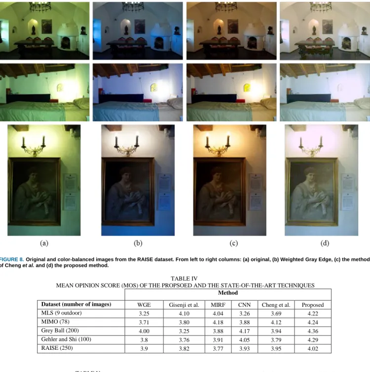
Fig. 8 shows the sample images and the resulting color- balanced images that were obtained using the proposed method and two state-of-the-art techniques, namely Weighted Gray Edge and the method of Cheng et al. (the images of the Weighted Gray Edge and Cheng et al.’s
that the presented images are in standard RGB (sRGB) format (Gehler’s publicly available code was used to convert the format of the images [48]). Column ‘a’ of Fig. 8 shows the input images, which suffer from an extreme presence of green color cast. Column ‘b’ of Fig. 8 shows WGE’s images. These images have turned bluish in nature. The Cheng et al.
method’s images are shown in Fig. 8 column ‘c’. These images demonstrate superior color constancy compared to the WGE images. However, the illuminant colors of the 1st and the 3rd images from the top are yellow-shifted relative to the canonical case. The proposed technique’s images are shown in column ‘d’. These images have the lowest color casting in comparison to the images of WGE and the method of Cheng et al. This implies that the proposed method outperforms these two state-of-the-art methods.
To evaluate the objective performance of the proposed method, the MIMO image dataset and 9 outdoor images of the Multiple Light Source dataset were chosen. The proposed method, state-of-the-art techniques (the method of Gisenji et al. [23], MIRF [24], Gray Pixel [34], Exemplar [38]) and other existing methods (Max-RGB, Gray World, Gray Edge 1-2 ) were used to generate objective results. The average mean and median angular errors of the images that were obtained by Gray world, Max_RGB, Gray Edge-1, Gray Edge-2, the method of Gijsenij et al., MIRF, GP (std) (M = 2), GP (std) (M = 4) and the proposed method for real and laboratory images of the MIMO dataset were calculated and tabulated in Table 2. According to Table 2, the proposed method’s average mean angular error is the lowest for the ‘real-world’ images of the MIMO dataset. However, the median error of the proposed method is slightly higher than that of the method of Gijsenij et al., MIRF, GP (std) (M = 2) and GP (std) (M = 4). From Table 2, the proposed method’s average mean and median angular errors are the lowest for all of the ‘laboratory’ images of the MIMO dataset. This finding confirms that the proposed technique generates almost the highest objective color constancy.
Table 3 shows the median angular errors of the proposed method, Max-RGB, Gray World, Gray Edge 1-2, the method of Gisenji et al. and Exemplar [38] using 9 outdoor images of the Multiple Light Source dataset [23].
A Mean Opinion Score (MOS) assessment on a selection of images from the five above mentioned datasets was conducted. The corrected images of the proposed and the state-of-the-art techniques were subjectively assessed by 10 independent observers. The observers scored the color constancy of each image from 1 to 5, where 1 to 5 represent the lowest to highest color constancy. The average MOS scores for images of different techniques were tabulated in Table 4. From Table 4, it can be seen that the proposed method’s images have the highest MOS compared to other techniques’ images.
The performance of the proposed method for different
FIGURE 5. A sample image from Gehler and Shi dataset [48]: (a) original
image, (b) ground truth, (c) Gray Edge-1 [11], (d) Weighted Gray Edge [12], (e) CNN [28] and (f) proposed method.
TABLE II
AVERAGE MEAN AND MEDIAN ANGULAR ERRORS OF STATE-OF-THE-ART AND THE PROPOSED METHOD FOR REAL AND
LABORATORY IMAGES FROM THE MIMO DATASET
MIMO (real) MIMO (lab)
Method Mean Median Mean Median
Gray world 4.2° 5.2° 3.2° 2.9° Max_RGB 5.6° 6.8° 7.8° 7.6° Gray Edge-1 3.9° 5.3° 3.1° 2.8° Gray Edge-2 4.7° 6.0° 3.2° 2.9° Gijsenij et al. 4.2° 3.8° 4.2° 4.8° MIRF 4.1° 3.3° 2.6° 2.6° GP (std) (M = 2) 5.74° 3.28° 2.53° 3.13° GP (std) (M = 4) 5.59° 3.44° 2.27° 2.94° Proposed (NS=4) 3.82° 3.89° 1.6° 1.5°
numbers of segments (2 to 6 with step of 1) on images of the MIMO and MLS datasets was investigated, and the results were tabulated in Table 5. From this table it can be seen that the proposed method gives the highest performance when the number of segments is set to 4.
10 VOLUME XX, 2017
FIGURE 6. A sample image from the Gehler and Shi dataset [45]: (a) original image, (b) ground truth, (c) Gray Edge-1 [11], (d) Weighted Gray Edge [12], (e) CNN [28] and (f) the proposed method.
3.1. ARGUMENT ON OBJECTIVE ASSESSMENT IN TERMS OF HUMAN PERCEPTION
The use of objective measures, e.g., angular error, to assess the color constancy of an image is debatable, as they are not always consistent with subjective evaluations. There are two
FIGURE 7. Original and color-balanced images: a) original image from
Gray Ball dataset, b) Gray World, c) Max-RGB (White Patch), d) Shades of Gray, e) 1st-Order Gray Edge, f) 2nd-Order Gray Edge, g) Weighted Gray Edge, and h) the proposed method.
TABLE III
MEDIAN ANGULAR ERRORS FOR 9 OUTDOOR IMAGES FROM THE MULTIPLE LIGHT SOURCE DATASET
Method Median error
Max_RGB 7.8°
Gray World 8.9°
Gray Edge-1 6.4°
Gray Edge-2 5.0°
Gisenji et al. 5.1°
Exemplar based (multi_illu) 4.3°
Proposed (NS=4) 4.0
potential shortcomings of using angular error as an assessment measure. First, the underlying distributions of image colors are not adequately summarized by the mean or median value of the angular error. Second, lower mean or median angular errors are not sufficient to determine the best-performing algorithm as the images have non- symmetric color distributions [50]. These shortcomings are identified by the Wilcoxson Sign test [51], which is used in
FIGURE 8. Original and color-balanced images from the RAISE dataset. From left to right columns: (a) original, (b) Weighted Gray Edge, (c) the method of Cheng et al. and (d) the proposed method.
TABLE IV
MEAN OPINION SCORE (MOS) OF THE PROPSOED AND THE STATE-OF-THE-ART TECHNIQUES Method
Dataset (number of images) WGE Gisenji et al. MIRF CNN Cheng et al. Proposed
MLS (9 outdoor) 3.25 4.10 4.04 3.26 3.69 4.22
MIMO (78) 3.71 3.80 4.18 3.88 4.12 4.24
Grey Ball (200) 4.00 3.25 3.88 4.17 3.94 4.36
Gehler and Shi (100) 3.8 3.76 3.91 4.05 3.79 4.29
RAISE (250) 3.9 3.82 3.77 3.93 3.95 4.02
TABLE V
ANGLUAR ERROR OF THE PROPSOED METHOD FOR DIFFERENT NUMBER OF SEGMENTS Angular Error Number of Segments (NS) MIMO (real) MIMO (lab) MLS (outdoor) 2 6.3 6.7 8.4 3 6.1 5.9 7.5 4 3.8 1.5 4.0 5 5.6 2.9 5.9 6 8.1 7.2 6.8
[34, 36, 52], where it is shown empirically that the performance of algorithm A is significantly better than that of algorithm B, while the angular error gives the opposite result. In addition, an investigation by Finlayson and Zakizadeh [53] shows that the angular error is not a reliable method for assessing the color constancy of an image. Different angular errors can result from the same scene if it is viewed under different illuminations, even if they are color balanced with the same color constancy algorithm. However, despite the uncertainty in these correlations between the angular error and human perception, a very similar result to visual perception can be achieved using angular error in some cases [54]. Nonetheless, human eyes are the most
12 VOLUME XX, 2017 reliable judge for measuring the color constancy of images,
which is undoubtedly accepted in the literature. Therefore, the subjective method was mainly used in this paper as a reliable color constancy assessment method.
IV. CONCLUSIONS
This paper presented a color constancy adjustment algorithm for images that are lit by single or multiple light sources. The proposed technique split the input image into multiple segments using the K-means++ algorithm. Each segment’s pixels were assessed in terms of whether they had enough color information to be used for image color constancy using the normalized average absolute difference values of their color components. The centroid and initial color constancy values for each selected segment were calculated using the Max-RGB algorithm. Finally, the color constancy weighting factors for each image pixel were calculated by combining the color constancies of all selected segments, which were weighted by the normalized Euclidian distances of the pixel from the centroids of the selected segments. This process enabled the method to balance the effects of the multiple illuminants on the color of each pixel. The results were generated using the images of five standard image datasets for single and multiple illuminants for both indoor and outdoor images. Experimental results showed that the proposed technique generates the best subjective results. The objective assessment showed that the proposed technique’s performance is highly comparable to other methods. However, in some cases, the objective quality may fall slightly below those of the state-of-the-art techniques.
REFERENCES
[1] G. D. Finlayson, P. A. T. Rey and E. Trezzi, "General lp constrained
approach for colour constancy," 2011 IEEE International Conference on Computer Vision Workshops (ICCV Workshops), Barcelona, 2011, pp. 790-797.
[2] F. J. Chang and S. C. Pei, "Color constancy via chromaticity neutralization: From single to multiple illuminants," 2013 IEEE International Symposium on Circuits and Systems (ISCAS2013), Beijing, 2013, pp. 2808-2811.
[3] S. Bianco, C. Cusano and R. Schettini, "Single and Multiple Illuminant Estimation Using Convolutional Neural Networks," in IEEE Transactions on Image Processing, vol. 26, no. 9, pp. 4347-4362, Sept. 2017.
[4] J. Simão, H. J. A. Schneebeli and R. F. Vassallo, "An Iterative Approach for Color Constancy," 2014 Joint Conference on Robotics: SBR-LARS Robotics Symposium and Robocontrol, Sao Carlos, 2014, pp. 130-135.
[5] Yanlin Qian, K. Chen, J. K. Kämäräinen, J. Nikkanen and J. Matas, "Deep structured-output regression learning for computational color constancy," 2016 23rd International Conference on Pattern Recognition (ICPR), Cancun, 2016, pp. 1899-1904.
[6] A. Gijsenij, T. Gevers, and J. Van de Weijer, "Computational Color Constancy: Survey and Experiments," in Image Processing, IEEE Transactions on, vol.20, no.9, pp.2475-2489, September 2011. [7] N. Banić, and S. Lončarić, "Color Cat: Remembering Colors for
Illumination Estimation," in IEEE Signal Processing Letters, vol. 22, no. 6, pp. 651-655, June 2015.
[8] G. Buchsbaum, “A spatial processor model for object colour perception,” Journal of the Franklin Institute, vol. 310, no. 1, pp. 1– 26, July 1980.
[9] E. Land, “The retinex theory of colour vision,” Scientific American, vol. 237, no. 6, pp. 108–128, December 1977.
[10] G.D. Finlayson, and E. Trezzi, “Shades of grey and colour constancy,”
Proc. IS&T/SID Color Imaging Conf., pp. 37-41, 2004.
[11] J. van de Weijer, T. Gevers, and A. Gijsenij, "Edge based colour constancy," IEEE Trans on Image Processing, pp.2 207-2217, 2007. [12] A. Gijsenij, T. Gevers, and J. Van de Weijer, "Improving Color
Constancy by Photometric Edge Weighting," IEEE Trans. on Pattern Analysis and Machine Intelligence, vol. 34(5):918-929, 2012. [13] D. Forsyth, “A novel algorithm for color constancy,” International
Journal of Computer Vision, vol. 5, no. 1, pp. 5–36, 1990.
[14] G. Finalyson, “Color in perspective,” IEEE Transactions on Pattern Analysis and Machine Intelligence, vol. 18, no. 10, pp. 1034–1038, 1996.
[15] G. Finlayson and S. Hordley, “Improving gamut mapping color constancy,” IEEETransactions on Image Processing, vol. 9, no. 10, pp. 1774–1783, 2000.
[16] H. Lee, “Method for computing the scene-illuminant chromaticity from specular highlights,” Journal of the Optical Society of America A, vol. 3, no. 10, pp. 1694–1699, 1986.
[17] S. Tominaga and B. Wandell, “Standard surface-reflectance model and illuminant estimation,” Journal of the Optical Society of America A, vol. 6, no. 4, pp. 576–584, 1989.
[18] G. Schaefer, S. Hordley, and G. Finlayson, "A combined physical and statistical approach to colour constancy,” IEEE Computer Society Conference on Computer Vision and Pattern Recognition, pp. 148-153 vol. 1, 2005.
[19] Y. Y. Liao, J. S. Lin and S. C. Tai, "Color balance algorithm with Zone system in color image correction," 2011 6th International Conference on Computer Sciences and Convergence Information Technology (ICCIT), Seogwipo, 2011, pp. 167-172.
[20] N. Xu, W. Lin, Y. Zhou, Y. Chen, Z. Chen and H. Li, "A new global-based video enhancement algorithm by fusing features of multiple region-of-interests," 2011 Visual Communications and Image Processing (VCIP), Tainan, 2011, pp. 1-4.
[21] Y. Chen, W. Lin, C. Zhang, Z. Chen, N. Xu and J. Xie, "Intra-and-Inter-Constraint-Based Video Enhancement Based on Piecewise Tone Mapping," in IEEE Transactions on Circuits and Systems for Video Technology, vol. 23, no. 1, pp. 74-82, Jan. 2013.
[22] C. Riess, E. Eibenberger and E. Angelopoulou, "Illuminant color estimation for real-world mixed-illuminant scenes," 2011 IEEE International Conference on Computer Vision Workshops (ICCV Workshops), Barcelona, 2011, pp. 782-789.
[23] A. Gijsenij, R. Lu and T. Gevers, "Color Constancy for Multiple Light Sources," in IEEE Transactions on Image Processing, vol. 21, no. 2, pp. 697-707, Feb.2012.
[24] S. Beigpour, C. Riess, J. van de Weijer, and E. Angelopoulou, "Multi-Illuminant Estimation with Conditional Random Fields," in IEEE Transactions on Image Processing, vol. 23, no. 1, pp. 83-96, Jan. 2014.
[25] M. Bleier et al., "Color constancy and non-uniform illumination: Can existing algorithms work?", IEEE International Conference on Computer Vision Workshops, pp. 774-781, 2011.
[26] P. M. O. Veksler, Y. Boykov. Superpixels and Supervoxels in an Energy Optimization Framework. In European Conference on Computer Vision, Sept. 2010.
[27] J. T. Barron, "Convolutional Color Constancy," 2015 IEEE International Conference on Computer Vision (ICCV), Santiago, 2015, pp. 379-387.
[28] S. Bianco, C. Cusano and R. Schettini, "Color constancy using CNNs,"
2015 IEEE Conference on Computer Vision and Pattern Recognition Workshops (CVPRW), Boston, MA, 2015, pp. 81-89.
[29] D. Fourure, R. Emonet, E. Fromont, D. Muselet, A. Trémeau, and C. Wolf, "Mixed pooling neural networks for color constancy," IEEE International Conference on Image Processing, Phoenix, AZ, pp. 3997-4001, 2016.
[30] S. B. Gao, K. F. Yang, C. Y. Li and Y. J. Li, "Color Constancy Using Double-Opponency," in IEEE Transactions on Pattern Analysis and Machine Intelligence, vol. 37, no. 10, pp. 1973-1985, Oct. 1 2015. [31] X. S. Zhang, S. B. Gao, R. X. Li, X. Y. Du, C. Y. Li and Y. J. Li, "A
Retinal Mechanism Inspired Color Constancy Model," in IEEE Transactions on Image Processing, vol. 25, no. 3, pp. 1219-1232, March 2016.
[32] A. Akbarinia and C. A. Parraga, "Colour Constancy Beyond the Classical Receptive Field," in IEEE Transactions on Pattern Analysis and Machine Intelligence, vol. PP, no. 99, pp. 1-1.
[33] Im, J., Kim, D., Jung, J., Kim, T., Paik, J., "Dark channel prior-based white point estimation for automatic white balance," Consumer Electronics (ICCE), 2014 IEEE International Conference on , vol., no., pp.123,124, 10-13 Jan. 2014.
[34] K. F. Yang, S. B. Gao and Y. J. Li, "Efficient illuminant estimation for color constancy using grey pixels," 2015 IEEE Conference on Computer Vision and Pattern Recognition (CVPR), Boston, MA, 2015, pp. 2254-2263.
[35] B. Mazin, J. Delon and Y. Gousseau, "Estimation of Illuminants From Projections on the Planckian Locus," in IEEE Transactions on Image Processing, vol. 24, no. 6, pp. 1944-1955, June 2015.
[36] S. Bianco and R. Schettini, "Adaptive Color Constancy Using Faces," in IEEE Transactions on Pattern Analysis and Machine Intelligence, vol. 36, no. 8, pp. 1505-1518, Aug. 2014.
[37] N. Elfiky, T. Gevers, A. Gijsenij and J. Gonzàlez, "Color Constancy Using 3D Scene Geometry Derived From a Single Image," in IEEE Transactions on Image Processing, vol. 23, no. 9, pp. 3855-3868, Sept. 2014.
[38] H. R. V. Joze and M. S. Drew, "Exemplar-Based Color Constancy and Multiple Illumination," in IEEE Transactions on Pattern Analysis and Machine Intelligence, vol. 36, no. 5, pp. 860-873, May 2014. [39] L. Mutimbu and A. Robles-Kelly, "Multiple Illuminant Color
Estimation via Statistical Inference on Factor Graphs," in IEEE Transactions on Image Processing, vol. 25, no. 11, pp. 5383-5396, Nov. 2016.
[40] G. D. Finlayson, "Corrected-Moment Illuminant Estimation," 2013 IEEE International Conference on Computer Vision, Sydney, VIC, 2013, pp. 1904-1911.
[41] D. Cheng, B. Price, S. Cohen and M. S. Brown, "Beyond White: Ground Truth Colors for Color Constancy Correction," 2015 IEEE International Conference on Computer Vision (ICCV), Santiago, 2015, pp. 298-306.
[42] D. Cheng, A. Kamel, B. Price, S. Cohen and M. S. Brown, "Two Illuminant Estimation and User Correction Preference," 2016 IEEE Conference on Computer Vision and Pattern Recognition (CVPR), Las Vegas, NV, 2016, pp. 469-477.
[43] M. A. Hussain, A. S. Akbari and B. Mallik, "Colour constancy using sub-blocks of the image," 2016 International Conference on Signals and Electronic Systems (ICSES), Krakow, pp. 113-117, 2016. [44] M. A. Hussain, A. S. Akbari and A. Ghaffari, "Colour Constancy
Using K-Means Clustering Algorithm," 2016 9th International Conference on Developments in eSystems Engineering (DeSE), Liverpool, pp. 283-288, 2016.
[45] M. A. Hussain and A. S. Akbari, "Max-RGB Based Colour Constancy Using the Sub-blocks of the Image," 2016 9th International
Conference on Developments in eSystems Engineering (DeSE), Liverpool, pp. 289-294, 2016.
[46] D. Arthur, S, Vassilvitskii, “K-means++: The Advantages of Careful
Seeding”, Proceedings of the Eighteenth Annual ACM-SIAM Symposium on Discrete Algorithms, pp. 1027–1035, 2007 .
[47] F. Ciurea, and B. Funt, “A Large Image Database for Color Constancy Research”, Proceedings of the Imaging Science and Technology Eleventh Color Imaging Conference, pp. 160-164, 2003.
[48] P. Gehler, C. Rother, A. Blake, T. Sharp, and T. Minka, "Bayesian colour constancy revisited," IEEE Conference on Computer Vision and Pattern Recognition (CVPR), pp. 1-8, June 2008.
[49] D.T. Dang-Nguyen, C. Pasquini, V. Conotter, G. Boato, “RAISE – A Raw Images Dataset for Digital Image Forensics”, ACM Multimedia Systems, Portland, Oregon, March 18-20, 2015 .
[50] S. D. Hordley and G. D. Finlayson, "Re-evaluating colour constancy algorithms," Proceedings of the 17th International Conference on Pattern Recognition, 2004. ICPR 2004., pp. 76-79 Vol.1, 2004. [51] F. Wilcoxon, “Individual Comparisons by Ranking Methods”,
Biometrics Bulletin , Vol. 1, No. 6, pp. 80-83, 1945.
[52] L. Shi, W. Xiong, and B. Funt, “Illumination estimation via thin-plate spline interpolation”, Journal of the Optical Society of America, Vol. 28, Issue 5, pp. 940-948, 2011.
[53] G. D. Finlayson, R. Zakizadeh and A. Gijsenij, "The Reproduction Angular Error for Evaluating the Performance of Illuminant Estimation Algorithms," in IEEE Transactions on Pattern Analysis and Machine Intelligence, vol. 39, no. 7, pp. 1482-1488, July 1 2017. [54] A. Gijsenij, T. Gevers, and M.P. Lucassen, “Perceptual Analysis of Distance Measures for Color Constancy Algorithms,” J. Optical Soc. of Am. A, vol. 26, no. 10, pp. 2243-2256, 2009.
MD AKMOL HUSSAIN is pursuing his PhD at
Leeds Beckett University, UK. He received a B.Eng. degree in Electronics and Communication from University of Wolverhampton in 2011 and a Post-Graduate Certificate (Mainly by Research) from the University of Gloucestershire in 2014. His research interests include computer vision, image processing and image forensics.
DR. AKBAR SHEIKH AKBARI is a Senior
Lecturer in School of Computing, Creative Technologies & Engineering at Leeds Beckett University. He has a BSc (Hons), MSc (distinction) and PhD in Electronic and Electrical Engineering. After completing his PhD at Strathclyde University, he joined Bristol University to work on an EPSRC project in stereo/multi-view video processing. He continued his career in industry, working on real-time embedded video analytics systems. His main research interests include signal processing, hyperspectral image processing, source camera identification, image/video forgery, image hashing, biometric identification techniques, assisted living technologies, compressive sensing, camera tracking using retro-reflective materials, standard and non-standard image/video codecs, e.g., H.264 and HEVC, multi-view image/video processing, color constancy techniques, resolution enhancement methods, edge detection in low-SNR environments and medical image processing.