ISSN: 2522-2465 (Online)
Indexing/Abstracting
Forecasting GDP Growth: Application of
Autoregressive Integrated Moving Average Model Author: Yesuf M. Awel1c
Affiliation: 1PhD, Economist-Consultant; P.O Box
101182, Addis Ababa, Ethiopia.
c Email: [email protected]
Submission: December 5, 2017 Acceptance: November 22, 2018 Article Information:
To cite this document
Awel, Y. M. (2018). Forecasting GDP Growth: Application of Autoregressive Integrated Moving Average Model. Empirical Economic Review, 1(2), 1-16.
The online version of this manuscript is available at
https://journals.umt.edu.pk/sbe/eer/volume1issue2.aspx
DOI: https://doi.org/10.29145/eer/12/010201
Additional Information
For Subscriptions Email: [email protected]
For further information, please visit
http://journals.umt.edu.pk/sbe/eer/Home.aspx Published by Department of Economics University of Management and Technology Lahore, Pakistan
This manuscript has been published under the terms of Creative Commons Attribution-ShareAlike 4.0 International
License (CC-BY SA). EER under this license lets others distribute, remix,
tweak, and build upon the work it publishes, even commercially, as long as
the authors of the original work are credited for the original creation and the
Contributions are distributed under the same license as original.
Forecasting GDP Growth: Application of
Autoregressive Integrated Moving Average Model
Yesuf M. Awel1 Abstract
This paper uses Box-Jenkins approach to model and forecast real GDP growth in Ethiopia. Such an approach could easily provide forecast for key macroeconomic variables in limited data environment. Based on the approach, the paper estimates Autoregressive Integrated Moving Average ARIMA (1,1,1) model and forecasts real GDP growth. Both the in-sample fit and pseudo-out of sample forecasts show that the ARIMA model’s performance are good and better than other forecasts.
Keywords: ARIMA, Box-Jenkins Approach,Ethiopia, Forecasting, Real GDP,
JEL Classifications: C53, E27
1PhD, Economist-Consultant; P.O Box 101182, Addis Ababa, Ethiopia. E-mail: [email protected]
1. Introduction
Economic forecasting is a common practice in economics. This is often done either using univariate time series or multivariate economic models. The univariate time series models are single variable based models that are simple and have less data requirements, while the multivariate (time series or large aggregate economic) models are relatively complex and are based on several economic assumptions. Macroeconometric models are largely guided by economic theory that covers major economic sectors, activities and policies in an economy. They are formulated in a theoretically consistent manner, satisfying economic identities for use in both forecasts and policy analysis. Nevertheless, they are data intensive and time consuming. Several countries in Africa are constrained by timely availability of longer series of data of major economic indicators. Thus, developing large macroeconomic models could be challenging so, in such cases, forecasting could be done using univariate time series models.
There are several empirical studies available that compare the forecast performance of time series models. In the US, Stock and Watson (1998) reported that linear univariate autoregressions and vector auto regressive (VAR) models perform well than nonlinear models in a wide range of US macroeconomic series. Eitrheim, Husebo, and Nymoen (1999) found that first difference VAR model produces more accurate forecasts than large macro model used by the central bank of Norway. Besides, Banerjee, and Marcellino (2006) indicated that univariate models are more robust than multivariate models. Edge, Kiley, and Laforte (2010) also reported that simple time series models such as VAR produce forecasts that outperform forecasts from large macro models.
Importantly, there is a trade-off between precision with which one can estimate parameters and the complexity of a model (Robertson & Tallman, 1999) and often macroeconomic data are available for short sample periods; hence, simple univariate or VAR models could be superior in forecasting than the large macro models. Therefore, in a data scarce environment, univariate time
series models can be used in lieu of large macroeconomic models for short term forecasting purposes.
Though not institutionalized and some are dated, there are a few macro models developed for the Ethiopian economy (See the review in Geda & Zerfu, 2004). However, the use of univariate time series models for forecasting seems to be missing. Moreover, the availability of long series of macroeconomic data is scarce for Ethiopia. The main aim of this study is to show the use of univariate time series model for forecasting in countries with limited data environment. Such approach is easier and could easily provide forecast for key macroeconomic variables such as GDP and inflation. The study uses real GDP data for Ethiopia covering the periods 1980-2014 drawn from World Development Indicators database (World Bank, 2015). GDP is a key aggregate indicator of the economic performance. It reveals the final value of all goods and services produced in an economy over a given period. Policy makers (monetary as well as fiscal) require forecasts to get an insight about the future trend of the economy and to respond timely.
This paper follows the Box and Jenkins (1976) approach to fit a univariate model that can be used to forecast real GDP growth. Since the real GDP series is expected to be non-stationary, the paper takes the first difference of the series and inspects its autocorrelation and partial autocorrelations to identify the values of AR and MA terms. Based on a combination of statistical significance of the estimated coefficients and goodness fit of the model based on Mean Square Error (MSE) and Akike Information Criteria (AIC), the study estimates an ARIMA (1,1,1) model to forecast real GDP growth in Ethiopia. Then, the paper assesses the forecast accuracy of the model using in-sample and pseudo-out of sample forecasts. According to the results the model performs well with in-sample forecast of Root Mean Square Error (RMSE)=0.063 and with pseudo-out of sample forecast (RMSE)=0.011, often the forecast undershoot actual realizations, comparing the model forecast with other forecasters (the IMF’s world economic outlook and the World Bank’s global economic prospects), the univariate model outperforms these forecasters given the low forecast errors. Hence, in data scarce environment, countries could use the available time
series data and fit univariate models to produce short-term forecasts to get a highlight of their economy in the future.
The paper is organized as follows. Section 2 discusses the Box-Jenkins methodology. Section 3 presents the econometric results and discusses the findings. The last section concludes and suggests further research directions.
2. Methodology
This study follows the Box and Jenkins (1976) methodology to develop a univariate time series forecasting model, often referred as Autoregressive Integrated Moving Average (ARIMA). The Box-Jenkins approach is based on Wold representation theorem that states every stationary time series has an infinite moving average (MA) representation. This means the future developments of the series can be expressed as a function of its past developments. The approach involves four stage iterative procedure (identification, estimation, diagnostic checking and forecasting) in developing a preferred model for forecasting.
The general ARIMA (p,d,q) model for a 𝑦𝑡 series integrated
of order 1 (d=1) is given as in equation (1). Where p is the AR term, d is the order of integration and q is the MA term.
∆𝑦𝑡 = 𝛼0+ 𝛼1∆𝑦𝑡−1+ 𝛼2∆𝑦𝑡−2+ ⋯ + 𝛼𝑝∆𝑦𝑡−𝑝+ 𝜃1𝜀𝑡−1+
𝜃2𝜀𝑡−2+ ⋯ + 𝜃𝑞𝜀𝑡−𝑞+ 𝜀𝑡 (1) 2.1. Model Identification
In the Box-Jenkins approach, the first stage is to examine the data and identify whether the series is stationary or not. That is testing for stationarity of the series using unit root tests (such as Augmented Dickey Fuller (ADF) and Phillips-Perron (PP) tests). Then, check for the appropriate AR(p) and MA(q) terms that should be included in the model. The paper uses the ACF and PACF to decide on the appropriate AR and MA terms. ACF is the correlation between 𝑦𝑡
and 𝑦𝑡−𝑞, while the PACF measures the partial correlation between
𝑦𝑡 and 𝑦𝑡−𝑝 accounting for the intermediate lags in between. The ACF that truncates at lag q suggest a MA(q), while the PACF that truncates at lag p suggest an AR(p).
2.2. Model Estimation
The second stage is estimating a class of ARIMA (p, d, q) models using maximum likelihood estimation and obtains the estimates of the coefficients of AR and MA terms. Using a combination of statistical significance of the estimated parameters, the overall model and Akike information Criteria (AIC) and Bayesian Information Criteria (BIC); the paper selects a preferred ARIMA model. AR is a model that expresses a variable in terms of its past values, while MA expresses the variable using its past errors. A series could be modeled using a combination of AR and MA. 2.3. Diagnostic Testing
The third stage is to diagnose the class of ARIMA models for adequacy. The study checks whether residuals of the model are white noise, not serially correlated and normally distributed. Specifically, the study uses the Portmanteau (Q) test for white noise, the ACF and PCF for checking the residuals serial correlation and the Jarqua-Bera normality test for checking the normality of the residuals.
2.4. Forecasting
Using the preferred model, this paper forecasts real GDP growth both in-sample and pseudo out of sample. The pseudo out of sample forecast is used, since the in-sample fit of the model could not well inform on the model’s forecast performance for future values out of the sample (Robertson & Tallman, 1999). Then, the paper assess the forecast accuracy of the model using Mean Absolute Error (MAE) and Root Mean Squared Error (RMSE). In-sample forecasting shows how the model fits the data in a given sample; while the pseudo out of sample forecast shows how the model forecasts for
future values which are out of the sample. Further, the study compares the forecast accuracy of the preferred model with other forecasts done for Ethiopia.
3. Econometric Results and Discussion
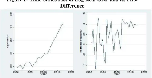
The study has used real GDP data from the WDI covering the years 1981-2014. Figure 1 plots the trend of log real GDP and its first difference (GDP growth). Over most of the sample period, real GDP shows a linear trend of growth perhaps implying the non-constant mean and variance of the series. There were some periods of decline in real GDP (for instance in 1984/85 due to extreme drought that affected the country; and 1991/92 due to aftermath of protracted civil war and beginning of transition). The growth rates oscillate between negative and positive values, though for most of the period are positive. Importantly, in the later periods (since 2004) the country registered impressive growth record averaging 11 percent per annum.
Figure 1: Time Series Plot of Log Real GDP and its First Difference
Source: World Development Indicator (WDI)
As discussed in the methodology section, the Box-Jenkins approach follows the iterative procedure of model identification, estimation, diagnostic checking and forecasting. The following subsections discuss the results of each stage.
3.1. Model Identification
The paper tests the stationarity of the real GDP series using ADF and PP tests. Table 1 shows that the log real GDP series (lrgdp) in levels is non-stationary under both Aaugmented Dickey Fuller (ADF) and Phillips Perron (PP) tests.
The log of GDP is taken to linearize the variable real GDP and improve the nature of the distribution into normality. However, the series becomes stationary in first difference (dlrgdp), since the null hypothesis of unit root is rejected at 1 percent level of significance in both ADF and PP tests as shown in Table 1. The results are consistent both under alternate specification (constant and constant with trend) as well as different lag lengths. Therefore, the paper uses the first difference in log real GDP in the ARIMA model.
Table 1: Stationarity Test of log of Real GDP (lrgdp) and its First Difference
ADF PP
Levels First difference Levels First difference
Lag
length Const.
Const.
& trend Const.
Const.
& trend Const.
Const.
& trend Const.
Const. & trend Lag 0 2.74 (1.00) -0.44 (0.49) -4.10*** (0.00) -5.12*** (0.00) 3.39 (1.00) -0.20 (0.99) -4.06*** (0.00) -5.14*** (0.00) Lag 1 1.99 (0.99) -0.61 (0.97) -3.73*** (0.00) -6.13*** (0.00) 2.64 (0.99) -0.49 (0.98) -4.14*** (0.000) -5.12*** (0.00) *** Statistically significant at 1 percent, values in parenthesis are MacKinnon approximate p-value
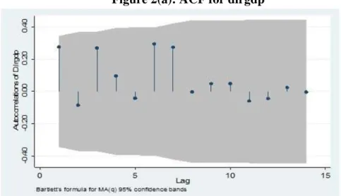
In order to determine the ARMA (p,q) model, the study has used the correlogram of autocorrelation function (ACF) and partial autocorrelation function (PACF) for dlrgdp. The value of p in AR(p) is determined by looking at the PACF that truncates at lag p; while the value of q in MA(q) is determined by considering ACF that truncates at lag q. The Ljung-Box Q-statistics tests the randomness of the series at a particular lag.
Table A1 at the appendix suggests that the value of p and q could be set to 1 at 10 percent level of significance, while Figures 2a-2b show that the values of p and q could be set to zero, respectively. However, the spikes in PACF at the third lag could affect the estimation results.
Figure 2(a): ACF for dlrgdp
Source: Calculated in Stata
Figure 2(b): PACF for dlrgdp
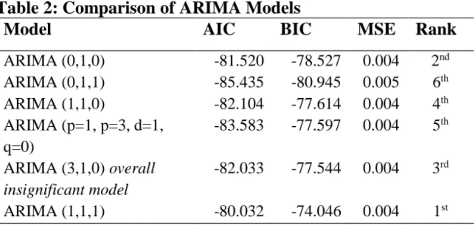
Given the limited number of observations and the yearly data at hand, the ARMA (p, q) could be set in to p=1 and q=1. Hence, the paper compares different combinations of ARIMA (p, 1, q) and selects a preferred model based on the information criteria (Akaike Information Criteria and Bayesian Information Criteria) and MSEs of each model. Table 2 shows that an ARIMA (1,1,1) is the preferred model given the low AIC and MSE.
Table 2: Comparison of ARIMA Models
Model AIC BIC MSE Rank
ARIMA (0,1,0) -81.520 -78.527 0.004 2nd ARIMA (0,1,1) -85.435 -80.945 0.005 6th ARIMA (1,1,0) -82.104 -77.614 0.004 4th ARIMA (p=1, p=3, d=1, q=0) -83.583 -77.597 0.004 5th ARIMA (3,1,0) overall insignificant model -82.033 -77.544 0.004 3rd ARIMA (1,1,1) -80.032 -74.046 0.004 1st 3.2. Model Estimation
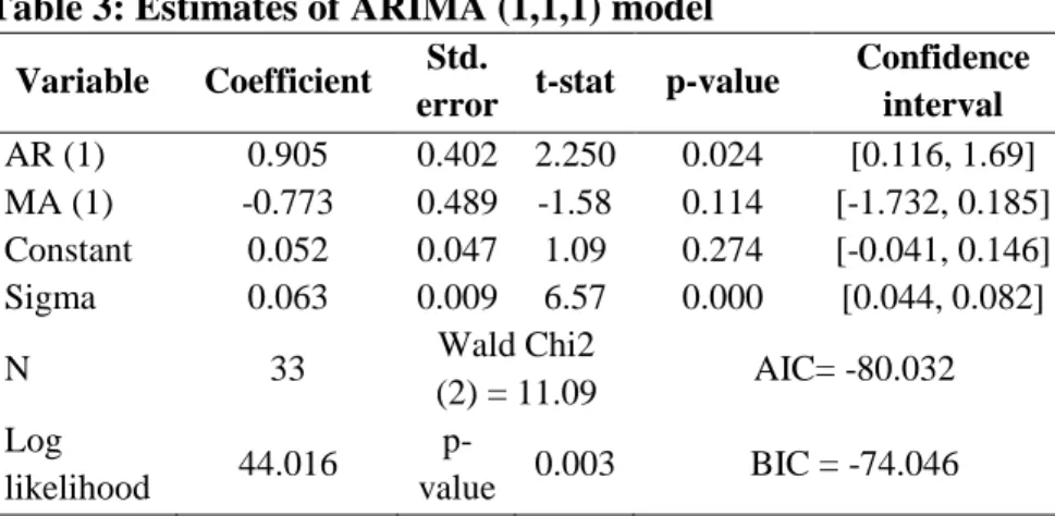
Table 3 presents the estimates of ARIMA (1,1,1) model, the preferred model. The AR (1) coefficient is statistically significant at 5 percent, while the MA (1) term is insignificant. Overall, the model is statistically significant (Wald Chi2 (2) =11.09, p-value = 0.003) with good model fit (MSE = 0.004). Though the series dlrgdp is stationary, the estimated coefficient of AR (1) is large perhaps due to the spike observed in the third lag of Figure 2b.
3.3. Diagnostic Checking
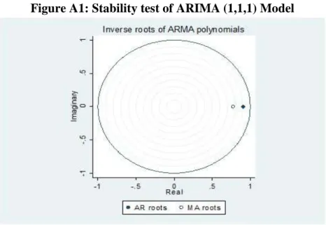
The paper diagnoses the estimated model for statistical significance and acceptability. First, the paper checks the stability of the ARIMA model using the inverse roots for AR and MA characteristics polynomials in Figure A1. The AR and MA roots, respectively are 0.9 and 0.77 that lie inside the unite circle implying stationarity and invertibility. Hence, the ARIMA (1,1,1) model is stable.
Table 3: Estimates of ARIMA (1,1,1) model
Variable Coefficient Std.
error t-stat p-value
Confidence interval AR (1) 0.905 0.402 2.250 0.024 [0.116, 1.69] MA (1) -0.773 0.489 -1.58 0.114 [-1.732, 0.185] Constant 0.052 0.047 1.09 0.274 [-0.041, 0.146] Sigma 0.063 0.009 6.57 0.000 [0.044, 0.082] N 33 Wald Chi2 (2) = 11.09 AIC= -80.032 Log likelihood 44.016 p-value 0.003 BIC = -74.046
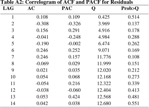
Second, the paper tests for the randomness (white noise), normality and autocorrelation of the residual. The Portmanteau Q-statistics test for white noise could not reject the null hypothesis of white noise residuals (Q-statistic = 12.67, p-value = 0.55). Further, the paper checks the normality of the residuals using the Jarque-Bera test and could not reject the normality of the residuals (Adjusted Chi-squared = 2.47, p-value=0.29). The paper also tests the autocorrelation of the residuals using Ljung-Box Q-statistics and provide the ACF and PACF graphs (see Figure 3a and 3b). The Ljung-Box Q-statistics in Table A2 at the appendix show that the null hypothesis of no autocorrelation of residuals are not rejected. Similarly, both ACF and PACF also show no autocorrelation of residuals. Overall, the residuals are white noise, normal (according to Figure A2) and serially non-autocorrelated. Hence, the diagnostic checks reveal that the ARIMA (1,1,1) model is statistically acceptable.
3.4. Forecasting
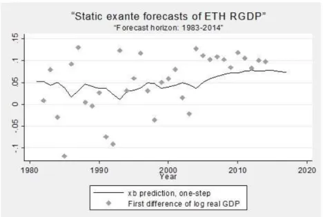
Based on ARIMA (1,1,1) model, the paper forecasts real GDP growth both in-sample and pseudo-out of sample. First, the paper estimates the ARIMA (1,1,1) model using data for 1981-2014 and get static forecast for the whole sample period. Second, the paper forecast out of sample for the period 2015-2017. Figure 4 shows the actual and static forecast for the sample period 1981-2014.
Figure 3(a): ACF of the ARIMA (1,1,1) Residuals
Source: Calculated in Stata
Based on both in-sample and pseudo-out of sample forecast, the study assesses the accuracy of the forecasts. Table 4 shows the MAE and RMSE. The forecast of the model is good with small forecast errors. Importantly, the pseudo-out of sample forecast errors are even smaller suggesting the good performance of the ARIMA (1,1,1) model.
Figure 3(b): PACF of the ARIMA (1,1,1) Residuals
Source: Calculated in Stata
The paper also compares the forecast accuracy of the univariate model with other forecasters, the IMF World Economic
Outlook (1990-2014) and the World Bank Global Economic Prospects (2007-2014). The forecasters’ accuracy is computed by comparing the year ahead forecast published in the reports and the actual realization the following year. The ARIMA (1,1,1) model outperforms both forecasters based on MAE and RMSE.
Figure 4: Actual and Static Forecast of Real GDP Growth
Source: Calculated in Stata
Table 4: Forecast Evaluation of ARIMA (1,1,1) and other Forecasters
Univariate model: ARIMA (1,1,1) WB-GEP IMF-WEO
In-sample forecast Pseudo-out of sample forecast Out of sample forecast Out of sample forecast MAE 0.0510 0.009 0.022 0.050 RMSE 0.0637 0.011 0.030 0.130 4. Conclusion
This paper aims to show the use of univariate time series model for forecasting in countries with limited data environment. Such approach is easier and could easily provide forecast for key
macroeconomic variables such as GDP and inflation. The paper uses real GDP data for Ethiopia covering the periods 1980-2014 drawn from World Development Indicators database (World Bank, 2015). The paper follows the Box and Jenkins (1976) approach to fit a univariate model that can be used to forecast GDP growth. Since the real GDP series is non-stationary, the paper takes the first difference of the series and inspect its autocorrelation and partial autocorrelations to identify the values of AR and MA terms. Based on a combination of statistical significance of the estimated coefficients and goodness fit of the model based on AIC and MSE, the paper estimates an ARIMA (1,1,1) model to forecast real GDP growth in Ethiopia. Then, it assesses the forecast accuracy of the model using in-sample and pseudo-out of sample forecasts. The preferred model performs well with in-sample forecast of RMSE=0.063 and pseudo-out of sample forecast of RMSE=0.011. Comparing the model forecast with other forecasters, the univariate model outperforms these forecasters given the low forecast errors.
Hence, in data scarce environment, countries could use the available time series data and fit univariate models to produce short-term forecasts to get a preview of their economy in the future. For further improving the modelling and forecasting of the GDP growth, the paper suggests further studies to investigate VAR models and compare them with univariate models and other forecasters.
References
Banerjee, A., & Marcellino, M. (2006). Are there any reliable leading indicators for the US inflation and GDP growth? International Journal of Forecasting, 22(1), 137-151. Box, G. E. P., & Jenkins, G. M. (1976). Time series analysis:
Fore-casting and control Holden-Day series in time series analysis. San Francisco, United States of America: Holden-Day.
Edge, R. M., Kiley, M. T., & Laforte, J. P. (2010). A comparison of forecast performance between Federal Reserve staff fore-casts, simple reduced-form models, and a DSGE model. Journal of Applied Econometrics, 25(4), 720-754.
Eitrheim, Ø., Husebø, T. A., & Nymoen, R. (1999). Equilibrium correction vs. differencing in macroeconometric forecasting. Economic Modelling, 16(4), 515-544.
Geda, A., & Zerfu, D. (2004). A review of macro modelling in Ethi-opia: (With lessons from published African models) (MOFED Working Paper No. MOFED-WP-01/2004). Retrieved from: http://alemayehu.com/Publication_MOF-ED/MOFED_AG&DZ_MacroReview_june2004.pdf
Robertson, J. C., & Tallman, W. E. (1999). Vector autoregressions: forecasting and reality. Economic Review-Federal Reserve Bank of Atlanta, 84(1), 4-18.
Stock, J. H., & Watson, M. W. (1998). A comparison of linear and nonlinear univariate models for forecasting macroeconomic time series (NBER Working Paper No. 6607). Retrieved from National Bureau of Economic Research website: http://www.nber.org/papers/w6607.pdf
World Bank. (2015). World development indicators database 2015. Retrieved from World Bank website: https://data.world-bank.org/products/wdi
Annexure - A
Table A1: Correlogram of ACF and PACF for dlrgdp
LAG AC PAC Q Prob>Q
1 0.274 0.279 2.723 0.098 2 -0.084 -0.178 2.991 0.224 3 0.268 0.416 5.774 0.123 4 0.095 -0.138 6.138 0.189 5 -0.042 0.119 6.211 0.286 6 0.294 0.311 9.913 0.128 7 0.274 0.161 13.25 0.066 8 -0.001 0.027 13.250 0.103 9 0.047 0.036 13.360 0.147 10 0.048 0.078 13.4780 0.198 11 -0.059 0.264 13.662 0.252 12 -0.044 -0.052 13.771 0.315 13 0.023 0.469 13.804 0.387 14 -0.003 0.034 13.805 0.464
Table A2: Correlogram of ACF and PACF for Residuals
LAG AC PAC Q Prob>Q
1 0.108 0.109 0.425 0.514 2 -0.308 -0.326 3.969 0.137 3 0.156 0.291 4.916 0.178 4 -0.041 -0.248 4.984 0.288 5 -0.190 -0.002 6.474 0.262 6 0.246 0.252 9.071 0.169 7 0.246 0.157 11.776 0.108 8 -0.069 0.029 11.999 0.151 9 0.021 0.035 12.020 0.212 10 0.054 0.068 12.168 0.273 11 -0.054 0.216 12.322 0.339 12 -0.038 -0.060 12.404 0.413 13 0.053 0.424 12.568 0.481 14 0.042 0.038 12.680 0.551
Annexure – B
Figure A1: Stability test of ARIMA (1,1,1) Model
Source: Calculated in Stata
Figure A2: Q-Q Plot for the Residuals