Building thermal load prediction through shallow machine learning and deep learning

Lawrence Berkeley National Laboratory

Recent Work

Title

Building thermal load prediction through shallow machine learning and deep learning

Permalink

Journal

ISSN

Authors

Publication Date

DOI

eScholarship.org Powered by the California Digital Library

DOI: 10.1016/j.apenergy.2020.114683

Building thermal load prediction through

shallow machine learning and deep

learning

Zhe Wang, Tianzhen Hong, Mary Ann Piette

Building Technology and Urban Systems Division

Lawrence Berkeley National Laboratory

Energy Technologies Area

April 2020

Disclaimer:

This document was prepared as an account of work sponsored by the United States Government. While this

document is believed to contain correct information, neither the United States Government nor any agency

thereof, nor the Regents of the University of California, nor any of their employees, makes any warranty,

express or implied, or assumes any legal responsibility for the accuracy, completeness, or usefulness of any

information, apparatus, product, or process disclosed, or represents that its use would not infringe privately

owned rights. Reference herein to any specific commercial product, process, or service by its trade name,

trademark, manufacturer, or otherwise, does not necessarily constitute or imply its endorsement,

recommendation, or favoring by the United States Government or any agency thereof, or the Regents of the

University of California. The views and opinions of authors expressed herein do not necessarily state or

reflect those of the United States Government or any agency thereof or the Regents of the University of

California.

Building thermal load prediction through shallow machine learning and

deep learning

Zhe Wang, Tianzhen Hong*_{, Mary Ann Piette}

Building Technology and Urban Systems Division Lawrence Berkeley National Laboratory One Cyclotron Road, Berkeley, CA 94720, USA

*_{Corresponding author: [email protected], (+1) 510-486-7082}

ABSTRACT

Building thermal load prediction informs the optimization of cooling plant and thermal energy storage. Physics-based prediction models of building thermal load are constrained by the model and input complexity. In this study, we developed 12 data-driven models (7 shallow learning, 2 deep learning, and 3 heuristic methods) to predict building thermal load and compared shallow machine learning and deep learning. The 12 prediction models were compared with the measured cooling demand. It was found XGBoost (Extreme Gradient Boost) and LSTM (Long Short Term Memory) provided the most accurate load prediction in the shallow and deep learning category, and both outperformed the best baseline model, which uses the previous day’s data for prediction. Then, we discussed how the prediction horizon and input uncertainty would influence the load prediction accuracy. Major conclusions are twofold: first, LSTM performs well in short-term prediction (1h ahead) but not in long short-term prediction (24h ahead), because the sequential information becomes less relevant and accordingly not so useful when the prediction horizon is long. Second, the presence of weather forecast uncertainty deteriorates XGBoost’s accuracy and favors LSTM, because the sequential information makes the model more robust to input uncertainty. Training the model with the uncertain rather than accurate weather data could enhance the model’s robustness. Our findings have two implications for practice. First, LSTM is recommended for short-term load prediction given that weather forecast uncertainty is unavoidable. Second, XGBoost is recommended for long term prediction, and the model should be trained with the presence of input uncertainty.

Keywords: building cooling load; prediction; weather forecast uncertainty; XGBoost; deep learning;

1. Introduction

The building sector is a major energy consumer and carbon emitter in modern society [1]. To reduce building energy usage and its associated carbon emissions, building thermal load prediction could play an important role. It has wide applications in HVAC control optimization [2], thermal energy storage operation [3], energy distribution system planning [4], and smart grid management [5] among others.

1.1 Previous work

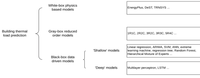
Because of its wide application, much research has been conducted to predict building thermal load, and those studies date back to the 1980s [6]. The approaches to forecasting building thermal load could be generally classified into three categories: white-box physics-based models, gray-box reduced-order models, and black-box data-driven models,1 _{as shown in Figure 1.}

Figure 1. Building thermal load prediction methods

White-box models predict building loads with detailed heat and mass transfer equations. Some mature software tools (such as EnergyPlus, Dest, and TRNSYS) are commercially available to set up white-box models [7]. To develop a detailed physics-based model, many detailed inputs are needed, and it is time-consuming to collect that information. More important, the uncertain and inaccurate inputs lead to a marked gap between the model results and reality [10].

Gray-box models simplify the building thermal dynamics to reduced order Resistance and Capacity (RC) models. Typically, the parameter values (Rs and Cs) are inferred from measured data (a.k.a. parameter identification) by minimizing the prediction errors, rather than from the specification of building physical parameters, as in the white-box model [11]. With new data available, the inferred parameters might change to reflect different building operations (window closing/opening) or material deterioration. In this regard, the gray-box model can be self-adaptive [12]. Models with different orders (how many Rs and Cs to represent

1 _{Strictly speaking, the studies reviewed in this section include cooling load prediction, heating load}

prediction, and building electricity usage prediction. In this review section, we focus more on the methods used, rather than strictly distinguish which variable is being predicted. This is a common practice in previous literature review articles like Li and Wen, 2014 [7], Zhao and Magoulès, 2012 [8], Amasyali and El-Gohary, 2016 [9], as building thermal load and electricity usage are highly correlated. Also, the task to predict building load and electricity usage share similar characteristics and implications.

the thermal zone or building envelope) have been proposed and studied, ranging from 1R1C [13], 2R2C [14], 3R2C [14], 3R3C [15], and 5R4C [15].2 _{Harb et al. compared RC models with different orders, and}

recommended the 4R2C model configuration [16]. A key shortcoming of a gray-box model is it only considers external heat gains, and overlooks internal heat gains. The gray-box models lack ways to identify and reflect the schedule and intensity change of occupant, lighting, and plug loads. As indicated in [17], the internal heat gains account for an increasingly higher proportion in modern buildings with a high-efficiency level of envelope.

Black-box models are purely data-driven; they predict building thermal load using historical data. As increasing amounts of data are monitored and collected, it becomes possible to learn the load patterns from historical data and use these learned patterns to make predictions. Early load forecast models were statistics-based models. For instance, in the 1980s, linear regression [18] (1984) and autoregressive integrated moving-average (ARIMA) [6] (1989) were applied to forecast building load. In subsequent years more complicated methods have been used. Some popular choices include support vector machine (SVM) [19]; artificial neural networks (ANN) [20]; extreme learning machine [21]; regression tree [22]; random forest [23]; and Hierarchical Mixture of Experts [24].

With the rapid development of deep learning in recent years, deep neural networks have been introduced as tools for load prediction. The major distinction between “shallow” and “deep” machine learning models lies in the number of linear or non-linear transformations the input data experiences before reaching an output. Deep models typically transform the inputs multiple times before delivering the outputs, while shallow models usually transform the inputs only one or two times. As a result, deep models can learn more complicated patterns, allowing end-to-end learning without manual feature engineering, and they perform well in tasks such as computer vision and sequential data analytics.

The most straightforward deep model is multilayer perceptron (MLP). MLP adds multiple hidden layers to an ordinary neural network to enhance its capability to learn more complicated patterns. Massana et al. applied MLP to predict the load for non-residential buildings [25]. However, MLP is not specially designed for time series data analytics, as it fails to capture and retain sequential information. Contrarily, a recurrent neural network (RNN), as a special form of the deep neural network, is specially designed to deal with time-series data. RNN is suitable for building load forecasts, as building load is essentially a time time-series. The long short term memory (LSTM) is a special form of RNN, which is designed to handle long sequential data. LSTM has been used successfully to forecast internal heat gains [17] or building energy usage [26]. However, to the best of the authors’ knowledge, LSTM has not been used for building thermal load prediction. Because many different algorithms are used to develop black-box load prediction models, a natural question is: “Is there a particular algorithm that is superior to others?” Li et al. compared SVM and ANN and found SVM performed better [27]. Guo et al. compared multivariable linear regression, SVM, ANN, and extreme learning machine and found extreme learning machine outperformed others [21]. Fan et al. compared seven machine learning algorithms (multiple linear regression, elastic net, random forests, gradient boosting machines, SVM, extreme gradient boosting, and deep neural network) and found extreme gradient boosting combined with deep auto-coding performed best [28]. Wang et al. compared LSTM and ARIMA and found

2 _{The model order might refer to different building components in different studies, and strictly speaking,}

are not comparable. For instance, the 2R2C and 3R2C model in reference [14] refer to internal thermal mass and external envelope, while the R3C3 and R5C4 mode in reference [15] refer to the whole thermal zone.

LSTM performs better than ARIMA in plug load prediction [29]. Rather than selecting the best predictor, ensembling multiple different predictors into one model could provide better generalization performance [23].

In addition to the prediction algorithms, determining what features should be used plays an important role in determining black-box model prediction accuracy. Time-related variables (hour of day, day type) are usually used, as they could reflect occupancy pattern, internal heat gains, and building usage schedule (like temperature set point) [28]. Outdoor weather variables (temperature and relative humidity) are also widely selected as features because weather conditions markedly influence the fresh air thermal load [30] and heat transfer through the building envelope. Some studies [21] used the return chilled water temperature as a predicting variable, as the return chilled water temperature could indicate real-time cooling demand and thermal mass of the current time step. However, the return chilled water temperature can only be used for short-term load prediction (on the scale of hours); it is not suitable for long-term forecasting (on the scale of days).

1.2 Research gap and objectives

As a rapidly developing area, new machine learning algorithms are being developed consistently. Though various literature has compared different algorithms, it is always worthwhile to investigate and reflect which algorithm performs best under the context of building load prediction. Additionally, to the best of the authors’ knowledge, some cutting-edge machine learning techniques (such as Extreme Gradient Boosting [XGBoost] and LSTM) have not been applied to forecast the building thermal load. To address this research gap, we aimed to predict building cooling load with two cutting-edge machine learning techniques—XGBoost and LSTM—which represent shallow machine learning and deep learning, respectively. XGBoost and LSTM were implemented with the XGBoost library [31] and Keras [32] in Python. These two tools are powerful, as most Kaggle competition3 _{winners used either the XGBoost library (for shallow machine learning) or}

Keras (for deep learning) [33]. The first objective of this study was to compare the performance of shallow and deep learning under the context of building load prediction.

The second research gap in past studies is how the input uncertainty would influence the performance and selection of machine learning algorithms. Under the context of building load prediction, weather data is one of the inputs that might be associated with uncertainty. For instance, to predict building load, we need to input weather forecast, which unavoidably has forecast uncertainty. The influence of weather forecast uncertainty is overlooked in previous studies. Given the existence of input uncertainty, for instance weather forecast uncertainty, which machine learning algorithm performs better and how to make the prediction model more robust is the second research question to be answered in this study.

2. Methodology

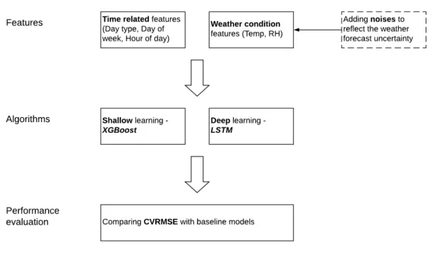
This study’s research roadmap is illustrated in Figure 2. The feature and the algorithm are two pillars of any data-driven models, and these will be discussed in Section 2.1 and Section 2.2. Section 2.3 details how we established the baseline models and introduced the evaluation index for model comparison. Prior to presenting the results, we introduce the case study building and the associated data collection process in Section 2.4.

3 _{See https://www.kaggle.com. This is the most popular and well-recognized competition in the machine}

Figure 2. Research roadmap

2.1 Algorithms

In this study, we compared shallow machine learning and deep learning for building load prediction. Deep learning involves multiple levels of representation and multiple layers of non-linear processing units, which is developing very fast in recent years and has successful applications in areas including computer vision and natural language processing. By contrast, all non-deep learning approaches can be classified as shallow learning. Both deep and shallow learning can deal with time-series data prediction, as in this case cooling load prediction. In deep learning, Recurrent Neural Network is designed to deal with sequential information, which is capable to extract and pass sequential information to the next time step. For shallow learning, sequential information is usually represented by time-related proxy variables such as hour of the day and day of the week.

For shallow machine learning, we compared Linear Regression, Ridge Regression, Lasso Regression, Elastic Net, Support Vector Machine (SVM) Random Forest, and Extreme Gradient Boosting (XGBoost); for deep learning, we compared vanilla Deep Neural Network and Long Short Term Memory (LSTM).

Linear Regression is the simplest machine learning algorithm. Ridge Regression adds regularization for 𝜄𝜄2

norm of the weight vector to the cost function, and Lasso Regression adds regularization for 𝜄𝜄1 norm. Elastic

Net simultaneously adds 𝜄𝜄2 and 𝜄𝜄1 norm regularization terms to the cost function. SVM is a powerful and

versatile machine learning algorithm that is capable of performing classification and regression tasks. Random Forest is an ensemble learning technique which is trained via the bagging method, i.e., building decision trees in a parallel way. In the deep learning category, we selected the vanilla Deep Neural Network, which inputs historical load and weather data for prediction without considering the sequential information. As XGBoost and LSTM are more advanced algorithms, which have not been widely used for building load prediction, we introduced these two algorithms in greater detail in this section: including the major ideas behind these two algorithms and how these ideas are implemented mathematically. The detailed

hyper-parameter tuning process for XGBoost and LSTM is presented in the appendix.

XGBoost

XGBoost is an ensemble learning technique, i.e., a predictor built out of many small predictors. XGBoost dominates recent machine learning and Kaggle competitions for structured or tabular data. As shown in [23], combining multiple predictors in a systematic way could enhance a model’s prediction accuracy and generalization capacity. Unlike random forest, which adds multiple predictors in a parallel way, XGBoost adds models sequentially; new models (𝑓𝑓𝑡𝑡 at iteration t) are built by focusing on the mistakes of the

predictors that come before it (the difference between the true label 𝑦𝑦𝑖𝑖 and the predicted label 𝑦𝑦�𝚤𝚤(𝑡𝑡−1) till

iteration (𝑡𝑡 −1)), aiming at minimizing the loss function 𝑙𝑙(𝑦𝑦𝑖𝑖,�𝑦𝑦�𝚤𝚤(𝑡𝑡−1)+𝑓𝑓𝑡𝑡(Χ𝑖𝑖)�), just as shown in Equation

(1). Through the mechanism of always trying to fix the prediction errors of prior models, XGBoost could improve its prediction accuracy.

ℒ<𝑡𝑡>_{=∑ 𝑙𝑙(𝑦𝑦}

𝑖𝑖,�𝑦𝑦�𝚤𝚤(𝑡𝑡−1)+𝑓𝑓𝑡𝑡(Χ𝑖𝑖)�) 𝑛𝑛

𝑖𝑖=1 +Ω(𝑓𝑓𝑡𝑡) (1)

Where, 𝑖𝑖 denotes the i-th sample to be predicted, 𝑛𝑛 is the total number of samples;

𝑡𝑡 denotes the t-th iteration; 𝑙𝑙(𝑦𝑦𝑖𝑖,𝑦𝑦�𝚤𝚤) is the loss-function between the true label 𝑦𝑦𝑖𝑖 and the

predicted label 𝑦𝑦�𝚤𝚤;

𝑓𝑓𝑡𝑡(Χ𝑖𝑖) is the base learner added at the t-th iteration, Χ𝑖𝑖 denotes the features for the i-th sample;

Ω(𝑓𝑓_𝑡𝑡) is the regularization term to avoid over-fitting; ℒ<𝑡𝑡> _{denotes the objective function at the t-th iteration}

However, the technique of repetitively building new models to focus on the mislabeled samples is likely to raise a concern of overfitting. XGBoost’s approach to solving this problem is to ensemble weak predictors rather than strong ones. A weak predictor is a simple prediction model that performs better than a random guess. A simple decision tree, with limited depths, is a good choice of individual predictors inside an ensemble learner, which is always found to outperform other options (multivariable regression, SVM, or even a decision tree with great depth). Additionally, a regularization term Ω(𝑓𝑓𝑡𝑡) is added to the objective

function ℒ<𝑡𝑡> _{to reject those base learner functions (𝑓𝑓}

𝑡𝑡) that might result in over-fitting.

Another key component of the ensemble learning algorithm is how the base learners (𝑓𝑓1 ~ 𝑓𝑓𝑡𝑡) are selected.

XGBoost applies second-order Taylor Expansion to approximate the value of loss functions, and uses the first order derivative and the second order derivative to help select the base learner 𝑓𝑓𝑡𝑡 [34].

To conclude, XGBoost is a decision tree-based ensemble machine learning algorithm that uses a gradient boosting framework. In this study, XGBoost is implemented using the XGBoost Library [31].

LSTM

LSTM is a special form of RNN, designed for handling long sequential data. Basic RNN architecture (Eq. 2 and Eq. 3) suffers from the problem of a vanishing or exploding gradient when the number of time steps (t) is large; however, this was successfully addressed by LSTM. Additionally, LSTM improves the information flow by introducing three additional gates: an update gate (Eq. 5), a forget gate (Eq. 6), and an output gate (Eq. 7); as well as two more cells: a candidate memory cell (Eq. 4) and a memory cell (Eq. 8) [35].

𝑎𝑎<𝑡𝑡>_{=𝑔𝑔(𝑊𝑊}

𝑎𝑎[𝑎𝑎<𝑡𝑡−1>,𝑥𝑥<𝑡𝑡>] +𝑏𝑏𝑎𝑎) (2)

𝑦𝑦<𝑡𝑡>_{=𝑔𝑔′�𝑊𝑊}

𝑦𝑦𝑎𝑎𝑎𝑎<𝑡𝑡>+𝑏𝑏𝑦𝑦� (3)

Where, 𝑔𝑔(𝑥𝑥) and 𝑔𝑔′(𝑥𝑥) are two activation functions; 𝑎𝑎<𝑡𝑡> _{is the activation value at time step t; 𝑥𝑥}<𝑡𝑡> _is

input at time step t; 𝑦𝑦<𝑡𝑡> _{is the output at time step t; 𝑊𝑊}

𝑎𝑎 and 𝑊𝑊𝑦𝑦𝑎𝑎 are weight matrices; 𝑏𝑏𝑎𝑎 and 𝑏𝑏𝑦𝑦 are

bias vectors; and [𝑎𝑎<𝑡𝑡−1>_,𝑥𝑥<𝑡𝑡>_{] denotes concatenate 𝑎𝑎}<𝑡𝑡−1> _{and 𝑥𝑥}<𝑡𝑡> _vertically.

In basic RNN, the memory passed to the next time step equals to the activation of the present time step (𝑎𝑎<𝑡𝑡−1>_{), as shown in Eq. 2. LSTM separates the memory cell from the output cell, and purposely adds a}

forget gate to calculate the update rate to determine how much memory needs to be passed to the next time step, adding flexibility to determine what and how much information should be passed to the next time step.

𝑐𝑐̃<𝑡𝑡>_{=𝑡𝑡𝑎𝑎𝑛𝑛ℎ(𝑊𝑊} 𝑐𝑐[𝑎𝑎<𝑡𝑡−1>,𝑥𝑥<𝑡𝑡>] +𝑏𝑏𝑐𝑐) (4) Γ𝑢𝑢=𝜎𝜎(𝑊𝑊𝑢𝑢[𝑎𝑎<𝑡𝑡−1>,𝑥𝑥<𝑡𝑡>] +𝑏𝑏𝑢𝑢) (5) Γ𝑓𝑓=𝜎𝜎�𝑊𝑊𝑓𝑓[𝑎𝑎<𝑡𝑡−1>,𝑥𝑥<𝑡𝑡>] +𝑏𝑏𝑓𝑓� (6) Γ𝑜𝑜=𝜎𝜎(𝑊𝑊𝑜𝑜[𝑎𝑎<𝑡𝑡−1>,𝑥𝑥<𝑡𝑡>] +𝑏𝑏𝑜𝑜) (7) 𝑐𝑐<𝑡𝑡>_=Γ 𝑢𝑢∗ 𝑐𝑐̃<𝑡𝑡>+Γ𝑓𝑓∗ 𝑐𝑐<𝑡𝑡−1> (8) 𝑎𝑎<𝑡𝑡>_=Γ 𝑜𝑜∗ 𝑡𝑡𝑎𝑎𝑛𝑛ℎ(𝑐𝑐<𝑡𝑡>) (9) 𝑦𝑦<𝑡𝑡>_{=𝑔𝑔′�𝑊𝑊} 𝑦𝑦𝑎𝑎𝑎𝑎<𝑡𝑡>+𝑏𝑏𝑦𝑦� (10)

Where, 𝑡𝑡𝑎𝑎𝑛𝑛ℎ(𝑥𝑥) is hyperbolic tangent function, as defined in Eq. 11; 𝜎𝜎(𝑥𝑥) is sigmoid function, as defined in Eq. 12; 𝑐𝑐̃<𝑡𝑡> _{is the memory candidate at time step t; 𝑐𝑐}<𝑡𝑡> _{is the memory value at time step t; Γ}

𝑢𝑢 is the

update gate; Γ𝑓𝑓 is the forget gate; Γo is the output gate; 𝑊𝑊𝑐𝑐 , 𝑊𝑊𝑢𝑢 , 𝑊𝑊𝑓𝑓 , and 𝑊𝑊𝑜𝑜 are weight matrices to

calculate the memory candidate, update gate, forget gate, output gate, respectively; 𝑏𝑏𝑐𝑐, 𝑏𝑏𝑢𝑢, 𝑏𝑏𝑓𝑓, and 𝑏𝑏𝑜𝑜 are

bias vectors to calculate the memory candidate, update gate, forget gate, output gate, respectively.

𝑡𝑡𝑎𝑎𝑛𝑛ℎ(𝑥𝑥) =𝑒𝑒_𝑒𝑒2𝑥𝑥2𝑥𝑥−1₊₁ (11)

𝜎𝜎(𝑥𝑥) =_𝑒𝑒𝑒𝑒𝑥𝑥₊₁𝑥𝑥 (12)

2.2 Features

Cooling load of a building is caused by internal heat gains and external heat gains [17]. Internal heat gains include the heat emission from occupants, miscellaneous electric loads, lighting, etc., which are influenced by the building operation schedule. Like in university campus buildings, internal heat gains are largely determined by the university calendar, such as class hours and school holidays. In this study, we selected time-related features – the hour of day, the day of week, and holiday – to predict internal heat gains. External heat gains include the cooling load to handle the ventilation air, and the heat transfer through external walls, roofs, windows, infiltration, etc., which are influenced by the outdoor weather condition. In this study, we selected outdoor air temperature and relative humidity to predict external heat gains.

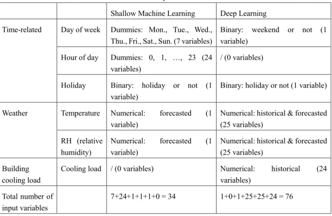
Table 1 presents and compares the input features for shallow and deep learning. Different algorithms have different inputs because they take different approaches to encode the time-related information. For shallow machine learning, time-related information is represented by the dummy variables of day of week and hour

of day. Contrarily, deep learning (e.g., LSTM) inputs historical data directly to reflect the sequential information. As shown in Table 1, LSTM consumes more input variables, and accordingly requires a longer training time.

Table 1. Input features

Shallow Machine Learning Deep Learning Time-related Day of week Dummies: Mon., Tue., Wed.,

Thu., Fri., Sat., Sun. (7 variables)

Binary: weekend or not (1 variable)

Hour of day Dummies: 0, 1, …, 23 (24 variables)

/ (0 variables)

Holiday Binary: holiday or not (1 variable)

Binary: holiday or not (1 variable)

Weather Temperature Numerical: forecasted (1 variable)

Numerical: historical & forecasted (25 variables)

RH (relative humidity)

Numerical: forecasted (1 variable)

Numerical: historical & forecasted (25 variables)

Building cooling load

Cooling load / (0 variables) Numerical: historical (24 variables)

Total number of input variables

7+24+1+1+1+0 = 34 1+0+1+25+25+24 = 76

As shown in Table 1, the weather forecast is needed to make a load prediction. Weather forecasts could not be exactly accurate for two reasons. First, the weather forecast itself is associated with prediction error and uncertainty. Second, the local climate of the target building and weather stations may be different. In most cases, the weather forecast is acquired by using the public API of online weather forecasting services such as Weather Underground (https://www.wunderground.com/) or Dark Sky (https://darksky.net), which predict the weather in the weather station location. It is unlikely that the target building is exactly at the same location as the weather station, which leads to another uncertainty.

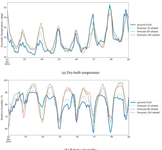
Figure 3 compares the forecast and real weather of a typical week. The weather forecast is from the API of Dark Sky, and the real weather data are measured by a local weather station placed in the target building. A difference can be observed in both the dry-bulb temperature and relative humidity forecast.

(a) Dry-bulb temperature

(b) Relative humidity

Figure 3. Comparison between the weather forecast and ground truth of a typical week

Figure 4 plots the key statistics and distribution of temperature and humidity forecast error of one-year data, comparing the weather forecast from Dark Sky to the ground truth measured by the local weather station. Though we presented both the mean and standard deviation of the forecast error, we only care about the standard deviation. Systematic bias of the prediction could be easily offset by adding or deducting a constant value, which could be easily learned by machine learning algorithms. However, the standard deviation of prediction error is associated with a random noise, which is unpredictable and poses additional uncertainty to the machine learning model. As shown in Figure 4, the forecast uncertainty, illustrated by the standard deviation of prediction error, increases with the prediction horizon. It could be observed that the mean error of temperature forecast is very small (less than 0.4o_{C) and would not increase with the prediction time}

horizon. However, the prediction is highly variant, and the prediction uncertainty would increase with a longer prediction time horizon.

(a) mean of temperature forecast error (b) standard deviation of temperature forecast error

(c) mean of relative humidity forecast error (d) standard deviation of relative humidity forecast error

(e) distribution of temperature forecast error (f) distribution of relative humidity forecast error

Figure 4. Key statistics and distribution of temperature and humidity forecast error

As observed in Figure 4(e) and 4(f), though the prediction error is skewed to the left for the temperature forecast and skewed to the right for the humidity forecast, the overall pattern is similar to the Gaussian distribution. We used three commonly used statistical test approaches to verify the null hypothesis that the prediction error follows Gaussian distribution: the Shapiro–Wilk test [36], D'Agostino's K-squared test [37], and the Anderson–Darling test [38]. The three tests were conducted with Python’s scipy.stats [39] Library. The p-values of both the temperature and humidity forecast under all three tests are very close to 0 (less than 10-10_{), indicating that we could not reject the null hypothesis that the prediction error follows the Gaussian}

distribution. Therefore, we proposed the weather forecast uncertainty model as shown in Eq. 13 and the coefficients shown in Table 2. As shown in Figure 4e and 4f, the forecast errors generated by Eq. 13 fit well

to the actual weather forecast errors.

𝑓𝑓𝑓𝑓𝑓𝑓𝑓𝑓𝑐𝑐𝑎𝑎𝑓𝑓𝑡𝑡_𝑓𝑓𝑓𝑓𝑓𝑓𝑓𝑓𝑓𝑓(𝑥𝑥) =_{√2𝜋𝜋𝜎𝜎}1 ₂𝑓𝑓−(𝑥𝑥−𝜇𝜇2𝜎𝜎2)2 (13)

Table 2. Key statistics for the weather forecast error model

Temperature prediction Relative humidity prediction

μ 0.6 4%

σ 1.5 12%

We did not distinguish different prediction horizons and utilized one set of (μ,σ) values because the forecast uncertainty does not vary significantly with the prediction horizon, as shown in Figure 4. To simulate the weather forecast uncertainty, we randomly sampled a value from Eq. 13 with coefficients from Table 2 and added this sampled noise to the ground truth of outdoor air temperature and humidity.

2.3 Baseline models

This section discusses our use of three conventional load forecast approaches as baseline models to evaluate how machine learning techniques could improve load prediction accuracy. The baseline models are selected based on the common practice in building operations.

Models 1 and 2: Persistence Daily and Weekly Algorithms

The persistence algorithm, which is also called the “naïve” forecast, utilizes the load of the previous time step (t) as the prediction for the next time step (t+1). To optimize the cooling plant and thermal storage tank through model predictive control (MPC), the load prediction horizon should be at least 24 hours ahead, so that the charging and discharging schedule of thermal storage can be optimized. Therefore, the first baseline model used the load of the previous day (given the same day type, working or non-working) as the prediction. This was named the persistence_daily model.

Considering the weekly periodicity of a building load, a natural idea is to utilize the load value of the previous week as the prediction for the next. To distinguish the second load prediction baseline model from the

persistence_daily model, it was named the persistence_weekly model.

Model 3: Rolling Window Algorithm

The rolling window forecast involves calculating a statistic, most likely the mean or the mode, of a fixed contiguous block of prior observations and using it as a forecast. In this study, the third baseline model we proposed used the mean of the load of the same hour and day of the week of the previous four weeks as the prediction. By averaging a couple of same-hour-same-day loads of previous weeks, random variations could be smoothed out, to enhance prediction robustness.

Comparison metrics

Another important step before comparing different forecasting models is to select a comparison index. In this study, we selected the coefficient of variation of the root mean square error (CVRMSE), defined in Eq. 13, which normalized the root mean square error by the mean value. CVRMSE is selected for two reasons. First, CVRMSE is a dimensionless indicator, which could facilitate cross-study comparisons because it filters out the scale effect. Second, CVRMSE is recommend by ASHRAE guideline 14 [40].

𝐶𝐶𝐶𝐶𝐶𝐶𝐶𝐶𝐶𝐶𝐶𝐶=�∑𝑖𝑖(𝑦𝑦� −𝑦𝑦𝚤𝚤 𝑖𝑖)2/𝑁𝑁

Where 𝑦𝑦�𝚤𝚤 and 𝑦𝑦𝑖𝑖 are the predicted and ground-truth values at time step i, and N is the number of total time

steps.

It is worthwhile to point out that some other evaluation indices are used in the existing literature, such as mean root mean square error (MRMSE) in Eq. 14 (used in studies [41], [27]) and mean absolute percentage error (MAPE) in Eq. 15 (used in studies [22], [25]). Those error evaluation indices are all presented in the form of percentages, and have similar definitions. However, they are not comparable. Given the same prediction, the error values reported in the form of MRMSE or MAPE would be less than the error value reported by CVRMSE. 𝐶𝐶𝐶𝐶𝐶𝐶𝐶𝐶𝐶𝐶=�∑(𝑦𝑦� −𝑦𝑦𝚤𝚤 𝑖𝑖 𝑦𝑦𝑖𝑖 ) 2 𝑖𝑖 /𝑁𝑁 (14) 𝐶𝐶𝑀𝑀𝑀𝑀𝐶𝐶=�∑ �𝑦𝑦� −𝑦𝑦𝚤𝚤 𝑖𝑖 𝑦𝑦𝑖𝑖 � 𝑖𝑖 /𝑁𝑁 (15)

2.4 Building used for the case study

In this study, we selected a university campus building located in California as our testbed. This building is mixed-used and provides laboratories, laboratory support spaces, teaching laboratories, and offices. This building has a floor area of about 175,000 square feet (16,000 square meters) and was awarded LEED-NC Gold. For privacy reasons, no more detailed information is provided.

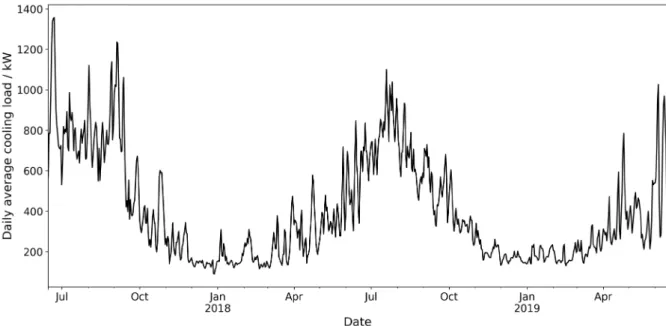
In the testbed building, we collected the chilled water supply temperature, chilled water return temperature, and the chiller water supply flowrate, to calculate the building cooling load. Additionally, we collected the outdoor dry-bulb temperature and relative humidity from the weather station located on the building roof. Figure 5 plots the two-year cooling load, which is used in this study, from June 15, 2017 to June 15, 2019.

3. Results

3.1 Performance of baseline models

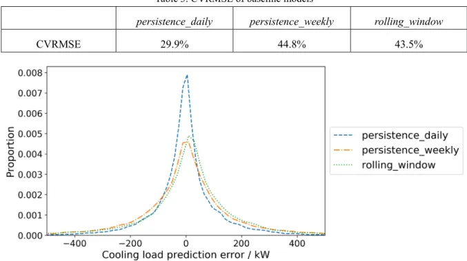
We compared the three baseline models and selected the one that performed the best for later comparison with the two machine learning models. As shown in Table 3 and Figure 6, the most naïve approach—using the load of the previous day as the forecast of the coming day—outperforms the other two baseline models. Therefore, the persistence_daily approach was selected as the baseline model of this study.

Table 3. CVRMSE of baseline models

persistence_daily persistence_weekly rolling_window

CVRMSE 29.9% 44.8% 43.5%

Figure 6. Distribution of prediction error of baseline models

Considering the daily periodical behavior of the occupant, lighting, and plug-load schedules, the value of the previous day is a good estimation for the internal heat gains of the coming day. As internal heat gains account for more than half of the building load in modern buildings [17], this naïve approach delivers a satisfactory prediction. However, another piece of information missed in the baseline model is the local weather, which is highly associated with the fresh air and external load through the envelope. Therefore, we used the forecasted weather as input features through machine learning techniques to enhance prediction accuracy. This process is described in the following sections.

3.2 Algorithm comparison

In this section, we compared different shallow machine learning and deep learning algorithms under the assumption that we have perfect knowledge about the weather data, i.e., the weather forecast is 100% accurate. In addition to the two algorithms introduced in Section 2.1, we compared seven more machine learning algorithms. In the shallow machine learning category, we compared Linear Regression, Ridge Regression, Lasso Regression, Elastic Net, Support Vector Machine (SVM) and Random Forest. Linear Regression is the simplest machine learning algorithm. Ridge Regression adds regularization for 𝜄𝜄2 norm

of the weight vector to the cost function, and Lasso Regression adds regularization for 𝜄𝜄1 norm. Elastic Net

versatile machine learning algorithm that is capable of performing classification and regression tasks. Random Forest is an ensemble learning technique which is trained via the bagging method, i.e., building decision trees in a parallel way. In the deep learning category, we compared vanilla Deep Neural Network, which inputs historical load and weather data for prediction without considering the sequential information. We first split the two-year hourly data into a training set and a testing set, with a ratio of 80 to 20. Then, we used the grid search tool provided by scikit-learn [42] , GridSearchCV, for hyper-parameter tuning. To avoid information leak, we put the 20% testing data aside, using the training dataset alone for the hyper-parameter tuning. After we found the best hyper-parameters with the grid search cross validation technique, we trained our model with the whole training dataset, and finally validated it on the test dataset. The hyper-parameter tuning process and the selected hyper-parameters are presented in the Appendix. The comparison result is shown in Table 4.

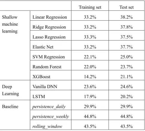
Table 4. CVRMSE of different models for 1h ahead load prediction

Training set Test set Shallow machine learning Linear Regression 33.2% 38.2% Ridge Regression 33.2% 37.8% Lasso Regression 33.3% 37.5% Elastic Net 33.2% 37.7% SVM Regression 22.1% 25.0% Random Forest 22.0% 23.7% XGBoost 14.2% 21.1% Deep Learning Vanilla DNN 23.6% 24.6% LSTM 17.9% 20.2% Baseline persistence_daily 29.9% 29.9% persistence_weekly 44.8% 44.8% rolling_window 43.5% 43.5%

As observed from Table 4, linear regressions with regularization terms (Ridge, Lasso and Elastic Net) have lower prediction errors in the test dataset. Adding regularization terms (either on 𝜄𝜄2 and 𝜄𝜄1) indeed enhances

the model’s capability to generalize to unseen datasets. Compared with baseline models, algorithms of linear regression family perform better than persistence_weekly and window, but worse than persistence_daily. Two more advanced shallow machine learning algorithms, SVM and Random Forest, improve the prediction accuracy compared with linear regression family algorithms and the best baseline. In the shallow machine learning algorithms, XGBoost performs the best, especially in the training set, which could be ascribed to the way how XGBoost was developed, i.e., new predictors are built to correct the mistakes of existing ones. However, similar to other sophisticated machine learning techniques, XGBoost is confronted with the overfitting problem. Its prediction accuracy on the test dataset is not as good as on the training dataset. In the deep learning category, LSTM outperforms vanilla DNN on both the training and the test datasets, by

taking better use of sequential information. Compared with complicated machine learning algorithms, baseline heuristic prediction models perform not too bad, considering its simplicity and the limited amount of data it requires.

Because XGBoost and LSTM are the best load prediction algorithm for shallow and deep learning respectively, we selected XGBoost and LSTM as the representative of each category for later analysis.

3.3 Prediction horizon

In this section, we selected XGBoost and LSTM as representative algorithms to discuss how the prediction horizon would influence the performance of shallow and deep learning. To facilitate prediction-based control, 24 hours ahead prediction is always needed. For instance, to optimize the operation of thermal energy storage, it is necessary to predict the cooling load of the next day.

For deep learning, as historical data (weather and building load) are needed as inputs, 1h ahead prediction is different from 24h ahead prediction. In 1h ahead prediction, we use historical trajectory 𝑞𝑞𝑡𝑡−23,𝑞𝑞𝑡𝑡−22,⋯,𝑞𝑞𝑡𝑡

and weather forecast 𝑇𝑇𝑡𝑡+1,𝐶𝐶𝑅𝑅𝑡𝑡+1 to predict cooling load 𝑞𝑞𝑡𝑡+1; in 24h ahead prediction, we use historical

trajectory 𝑞𝑞𝑡𝑡−23,𝑞𝑞𝑡𝑡−22,⋯,𝑞𝑞𝑡𝑡 and 𝑇𝑇𝑡𝑡+24,𝐶𝐶𝑅𝑅𝑡𝑡+24 to predict cooling load 𝑞𝑞𝑡𝑡+24 . Contrarily, for shallow

machine learning, historical data are not needed. We use weather forecast to predict load: 𝑇𝑇𝑡𝑡+1,𝐶𝐶𝑅𝑅𝑡𝑡+1 for

𝑞𝑞𝑡𝑡+1, and 𝑇𝑇𝑡𝑡+24,𝐶𝐶𝑅𝑅𝑡𝑡+24 for 𝑞𝑞𝑡𝑡+24. In this section, we assume we have perfect knowledge of the weather.

Therefore, for shallow machine learning, 1h ahead prediction is the same as 24h ahead prediction. In Figure 7, we differentiate 1h ahead prediction from 24h ahead prediction only for LSTM, but not for XGBoost.

(b) Load forecast by LSTM - 1h ahead

(d) Forecast on a typical week from the test dataset

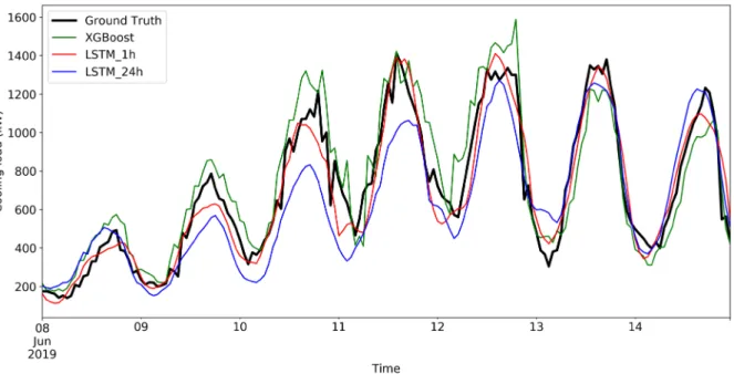
Figure 7. load forecasting results by LSTM and XGBoost for the whole time horizon and a typical week

Table 5. CVRMSE of different models

Training set Test set XGBoost 14.2% 21.1% LSTM_1h 17.9% 20.2% LSTM_24h 23.4% 31.9% Best Baseline 29.9% 29.9%

As shown in Figure 7(a) - 7(c), both the XGBoost and LSTM could track the general trend of the building load. If we zoom in on one-week data (figure 7(d)), it can be observed that LSTM delivers a smoother load curve. For 1h ahead prediction, XGBoost and LSTM both outperform the best baseline model by a large margin. However, for 24h ahead prediction, LSTM delivers a less accurate prediction compared with XGBoost and even the simple heuristic baseline model.

LSTM (and other sequential deep learning models such as RNN) uses the so-called ‘iterative approach’ to make 24h ahead prediction, i.e. using the historical data at time step 𝑡𝑡 −23,𝑡𝑡 −22,⋯,𝑡𝑡 to predict the time step 𝑡𝑡+ 1 ; and then using historical data 𝑡𝑡 −22,⋯,𝑡𝑡 and the predicted value at 𝑡𝑡+ 1 to make a prediction at the time step 𝑡𝑡+ 2; and iterate this process until the time step 𝑡𝑡+ 24 [28]. As we are using predicted information to make further predictions, the prediction error accumulated and propagated when the prediction horizon increases. As a result, LSTM performs better than XGBoost in short term (1h ahead) prediction, but worse in long term (24h ahead) prediction, as shown in Figure 7(d) and Table 5. This performance degradation could also be interpreted in another way. For 𝑡𝑡+ 1 prediction, the sequential information at time step 𝑡𝑡 −23,𝑡𝑡 −22,⋯,𝑡𝑡 is very relevant and therefore helpful. Contrarily, for 𝑡𝑡+ 24

therefore less helpful. As a result, 24ℎ ahead load prediction has a larger prediction error.

Generally speaking, deep learning does not perform as well as shallow machine learning, especially for long term prediction. A possible explanation is the sequential information that deep learning could leverage might be sufficiently captured by the time-related features (hour of day, and day type) and already reflected in XGBoost. The advantage of LSTM comes from its capability to capture sequential information, while the advantage of XGBoost comes from ensemble learning. In this case, the sequential information is no longer valuable as it could be captured by the time-related features. The advantage of deep learning might be less significant than the advantage of ensemble learning that XGBoost could leverage.

3.4 Effect of weather forecast uncertainty

The prediction results presented in the previous section utilized actual weather data for load prediction, which is a common practice in previous studies. However, actual weather data are not available when predicting building load for HVAC or thermal storage control. In this case, forecasted weather data, rather than actual weather data, are used for load prediction. The uncertainty of a weather forecast is seldom considered in previous studies. A natural question is how the weather forecast uncertainty would influence building load prediction accuracy, and which approach is more robust to weather forecast uncertainty. To answer those questions, we added a random noise (following the normal distribution of Eq. 13 and the parameters listed in Table 2) to the actual weather data to simulate the weather forecast uncertainty, and used the forecast weather data for load prediction.

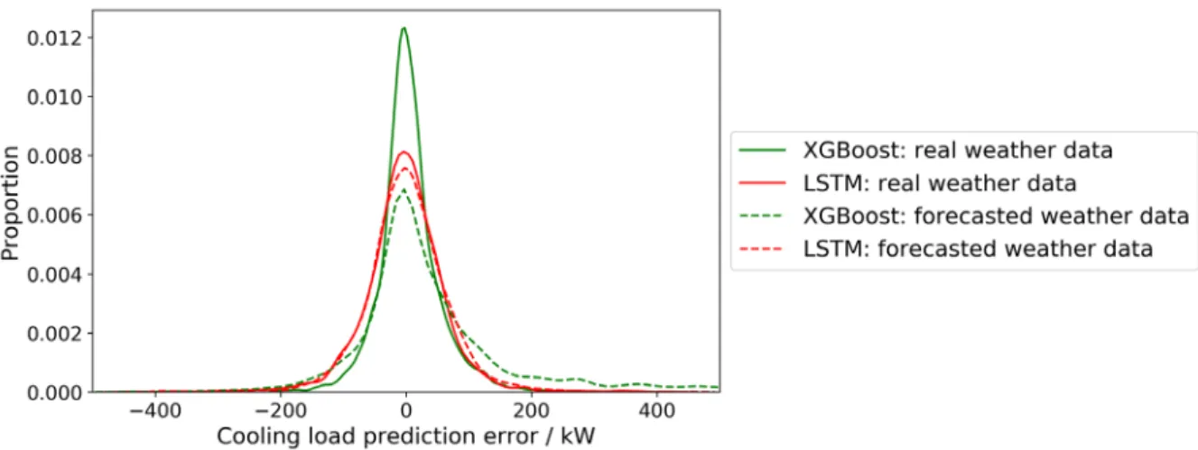
As shown in Figure 8(a), XGBoost is more sensitive to weather forecast uncertainty than LSTM. The presence of weather forecast uncertainty (1.5o_{C for temperature and 12% for relative humidity) markedly}

deteriorates XGBoost’s performance, making it less accurate than LSTM. Contrarily, LSTM is more robust to weather forecast uncertainty. The presence of weather forecast uncertainty only increases its CVRMSE by 1%. As a special form of recurrent neural network, the sequential information presented in LSTM helps to stabilize its prediction, making it less sensitive to weather forecast uncertainty. However, this sequential information is missing in shallow models such as XGBoost.

The next research question to answer is: given the existence of weather forecast uncertainty, should we train our model with the predicted weather or the real weather? As shown in Figure 4b, the model trained with the predicted weather outperforms the model trained with the real weather. Exposing the model to uncertain weather data at the training stage could make the model aware of the data uncertainty and gradually figure out a way to deal with this uncertainty during the training process. As shown in Table 6, training on the forecast weather data could reduce CVRMSE by 4.4%. Training the XGBoost model with predicted weather data makes the model less sensitive to weather forecast uncertainty.

(a) load prediction error with and without weather forecast uncertainty: model trained with real weather data and tested on forecasted weather data

(b) train XGBoost with forecast weather data Figure 8. Load forecasting with forecast weather data

Table 6. CVRMSE of prediction models

Weather forecast uncertainty not considered

(%)

Weather forecast uncertainty considered Train on real, test on

forecasted weather (%)

Train on forecast, test on forecasted weather (%) XGBoost 21.1 27.7 23.3 LSTM 20.2 21.2 21.0 Best Baseline 29.9 29.9 29.9 4. Discussion 4.1 Algorithm comparison

In this paper, we compared 12 approaches for load prediction: three heuristic methods, seven shallow machine learning algorithms, and two deep learning algorithms. XGBoost delivers the most accurate prediction in the shallow machine learning category, and LSTM performs the best in the deep learning

category. Support Vector Machine, Random Forest, and vanilla Deep Neural Network provide similar prediction accuracy. The above five algorithms outperform the best baseline model developed from heuristic approaches.

It is worthy to point out that the simple baseline algorithm actually performs pretty well, especially when the weather forecast uncertainty exists. The model simplicity and data efficiency of the heuristic baseline model make it easy to be implemented and maintained. Such a load prediction method might be adequate for projects with small scales and a limited budget.

4.2 Contribution and limitation

This study targeted building level cooling load prediction, which could be used widely to improve building efficiency, reduce operational cost, and enhance building-grid interaction. The major contributions of this study are twofold. First, we compared 12 algorithms from three load prediction approaches: heuristic method, shallow and deep learning, which has not been done systematically in previous studies. Second, we explored how the prediction horizon and input uncertainty influence load prediction accuracy and algorithm selection, which has been overlooked in existing literature. We documented the hyper-parameter tuning process and the selected hyper-parameters in the appendix to make the result reproducible and to save future researchers’ time.

A limitation of this study is that we did not include solar radiation in model inputs. Though solar radiation is correlated to and partially reflected by ambient temperature, adding solar radiation might enhance load prediction accuracy, especially for those buildings with a large window-to-wall ratio. In this study, solar radiation was not considered due to the absence of data. A comprehensive study on the selection of weather-related features, including but not limited to dry-bulb temperature, relative humidity (or dew point temperature, wet-bulb temperature), solar radiation intensity, and wind velocity, is needed for future studies. Additionally, in this study we used the Gaussian random noise to model the weather forecast error, which might not reflect the real behavior of weather forecast errors. Because even though the weather forecast errors follow Gaussian distribution, as shown in Figure 4(e) and Figure 4(f), the independent, identically distributed (i.i.d.) assumption of random noise might not hold. To find a better mathematical representation of weather forecast errors is worth more investigation.

Future studies will further test and refine the machine learning models to predict cooling loads of more buildings across different climate zones.

5. Conclusions

Building load prediction has wide applications in the fields of HVAC control, thermal storage operation, smart grid management, and others. There are three approaches for building load prediction: white-box physics-based models, gray-box reduced-order models, and black-box data-driven models. However, a white-box model requires a huge amount of input parameters, which could degrade with time and might be challenging to measure. A gray-box model overlooks the variation of internal heat gains. In this study, we applied a black-box model to predict building load. Twelve load prediction models have been developed and compared with the data collected from a campus building located in California.

It was found that Extreme Gradient Boosting (XGBoost) and Long Short Term Memory (LSTM) are the most accurate shallow and deep learning model, respectively. The CVRMSE of load prediction on the test dataset is 21.1% for XGBoost and 20.2% for LSTM. Both XGBoost and LSTM outperform the best baseline

model, which has a CVRMSE of 29.9%. Compared with results in the existing literature, XGBoost is also among the best for building load prediction.

We then discussed how the prediction horizon and input uncertainty influenced the load prediction accuracy and algorithm selection. LSTM performs better for short-term prediction and is more robust to input uncertainty. The sequential information retained by LSTM could help to insulate its prediction from an inaccurate weather forecast. XGBoost performs better for long-term prediction, because sequential information captured by LSTM might be less relevant, and accordingly less helpful for long time horizon prediction.

Our findings have three implications for practice. For projects with limited budgets and resources, the heuristic load prediction method is recommended due to its simplicity and data efficiency. For short term prediction, LSTM is recommended as it is more robust to input uncertainty. For long term prediction, XGBoost is recommended; it is suggested to train the XGBoost model with the predicted but not the real weather data, as exposing the model to input uncertainty at the training stage could enhance the model’s robustness.

Acknowledgments

This research was supported by the Assistant Secretary for Energy Efficiency and Renewable Energy, Office of Building Technologies of the United States Department of Energy, under Contract No. DE-AC02-05CH11231.

Appendix. Input features and hyper-parameter tuning for XGBoost and LSTM

One shortcoming of XGBoost is that there are so many hyper-parameters that need to be tuned, and a carefully tuned model could outperform the model with default settings by a large margin. We used the Grid Search Cross Validation technique to tune the XGBoost. Table A1 illustrates the searched and the selected hyper-parameters for XGBoost.

Table A1. Grid search hyper-parameter tuning for XGBoost

Hyper-parameters Description Searched Selected

objective Objective or loss function reg:squarederror n_estimators Number of estimators [100, 150, 200, 250] 200

gamma Minimum loss reduction required to make a further partition on a leaf node of the tree

[0.02, 0.05, 0.1, 0.15, 0.2, 0.25, 0.3]

0.02

learning_rate Step size shrinkage used in update to prevent overfitting

[0.02, 0.04, 0.06, 0.08, 0.1]

0.04

max_depth Maximum depth of a tree [5, 6, 7, 8, 9, 10] 8 min_child_weight Minimum sum of instance weight

(hessian) needed in a child

[2, 3, 4, 5, 6] 3

subsample Subsample ratio of the training instances [0.4, 0.5, 0.6, 0.7, 0.8, 0.9, 1.0]

0.5

colsamle_bytree Subsample ratio of columns when constructing each tree

[0.6, 0.7, 0.8, 0.9, 1.0]

1.0

lambda L2 regularization term on weights [0.1, 0.2, 0.5, 0.8, 1.1]

0.1

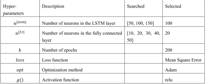
For LSTM, the number of tunable hyper-parameters is less than XGBoost. The searched and selected parameters are presented in Table A2.

Table A2. Grid search hyper-parameter tuning for LSTM

Hyper-parameters

Description Searched Selected

𝑛𝑛[𝑙𝑙𝑙𝑙𝑡𝑡𝑙𝑙] _{Number of neurons in the LSTM layer [50, 100, 150] 100}

𝑛𝑛[𝑓𝑓𝑐𝑐] _{Number of neurons in the fully connected}

layer

[10, 20, 30, 40, 50]

20

𝑘𝑘 Number of epochs 200

𝑙𝑙𝑓𝑓𝑓𝑓𝑓𝑓 Loss function Mean Square Error

𝑓𝑓𝑜𝑜𝑡𝑡 Optimization method Adam

For Ridge Regression, the searched and selected parameters are presented in Table A3.

Table A3. Grid search hyper-parameter tuning for Ridge Regression

Hyper-parameters

Description Searched Selected

α Regularization coefficient for 𝜄𝜄2 norm of

the weight vector

[1, 2, 5, 10, 20, 50, 100, 200]

50

For Lasso Regression, the searched and selected parameters are presented in Table A4.

Table A4. Grid search hyper-parameter tuning for Lasso Regression

Hyper-parameters

Description Searched Selected

β Regularization coefficient for 𝜄𝜄1 norm of

the weight vector

[0.1, 0.2, 0.5, 1, 2, 5, 10, 20]

2

For Elastic Net, the searched and selected parameters are presented in Table A5.

Table A5. Grid search hyper-parameter tuning for Elastic Net

Hyper-parameters

Description Searched Selected

α Regularization coefficient for 𝜄𝜄2 norm of

the weight vector

[1, 3, 10, 30, 100] 1

β Regularization coefficient for 𝜄𝜄1 norm of

the weight vector

[0.1, 0.3, 1, 3, 10] 1

For SVM Regression, the searched and selected parameters are presented in Table A6.

Table A6. Grid search hyper-parameter tuning for SVM Regression

Hyper-parameters

Description Searched Selected

kernel The kernel type used in the algorithm [‘linear’, ‘poly’, ‘rbf’, ‘sigmoid’]

‘rbf’

C Regularization parameter [0.1, 1, 10, 100, 1000]

100

epsilon Specifies the epsilon-tube within which no penalty is associated in the training loss function with points predicted within a distance epsilon from the actual value

For Random Forest, the searched and selected parameters are presented in Table A7.

Table A7. Grid search hyper-parameter tuning for Random Forest

Hyper-parameters Description Searched Selected n_estimators Number of decision trees in the RF [10,30,100,300] 100 max_depth The maximum depth of the tree [3, 4, 5, 6] 5 min_samples_split The minimum number of samples required

to split an internal node

[2, 3, 4, 5] 4

max_features The number of features to consider when looking for the best split

[‘auto’, ‘sqrt’] ‘auto’

For vanilla Deep Neural Network, the searched and selected parameters are presented in Table A8.

Table A7. Grid search hyper-parameter tuning for Deep Neural Network Layer

Hyper-parameters

Description Selected

1 𝑛𝑛[𝑓𝑓𝑐𝑐] _{Number of neurons 300}

𝑔𝑔() Activation function relu

2 _𝑛𝑛[𝑓𝑓𝑐𝑐] _{Number of neurons 100}

𝑔𝑔() Activation function relu

3 _𝑛𝑛[𝑓𝑓𝑐𝑐] _{Number of neurons 50}

𝑔𝑔() Activation function relu

/ 𝑘𝑘 Number of epochs 50

𝑙𝑙𝑓𝑓𝑓𝑓𝑓𝑓 Loss function Mean Square Error

𝑓𝑓𝑜𝑜𝑡𝑡 Optimization method Adam

References

[1] D. Ürge-Vorsatz, L. F. Cabeza, S. Serrano, C. Barreneche, and K. Petrichenko, “Heating and cooling energy trends and drivers in buildings,” Renew. Sustain. Energy Rev., vol. 41, pp. 85–98, Jan. 2015, doi: 10.1016/j.rser.2014.08.039.

[2] A. Kusiak and M. Li, “Cooling output optimization of an air handling unit,” Appl. Energy, vol. 87, no. 3, pp. 901–909, Mar. 2010, doi: 10.1016/j.apenergy.2009.06.010.

[3] N. Luo, T. Hong, H. Li, R. Jia, and W. Weng, “Data analytics and optimization of an ice-based energy storage system for commercial buildings,” Appl. Energy, vol. 204, pp. 459–475, Oct. 2017, doi: 10.1016/j.apenergy.2017.07.048.

buildings for the purpose of planning for mixed energy distribution systems,” Energy Build., vol. 40, no. 7, pp. 1124–1134, Jan. 2008, doi: 10.1016/j.enbuild.2007.10.014.

[5] X. Xue, S. Wang, Y. Sun, and F. Xiao, “An interactive building power demand management strategy for facilitating smart grid optimization,” Appl. Energy, vol. 116, pp. 297–310, Mar. 2014, doi: 10.1016/j.apenergy.2013.11.064.

[6] D. H. Spethmann, “Optimal control for cool storage,” ASHRAE Trans., vol. 95, pp. 710–721, 1989. [7] X. Li and J. Wen, “Review of building energy modeling for control and operation,” Renew. Sustain. Energy Rev., vol. 37, pp. 517–537, Sep. 2014, doi: 10.1016/j.rser.2014.05.056.

[8] H. Zhao and F. Magoulès, “A review on the prediction of building energy consumption,” Renew. Sustain. Energy Rev., vol. 16, no. 6, pp. 3586–3592, Aug. 2012, doi: 10.1016/j.rser.2012.02.049.

[9] K. Amasyali and N. M. El-Gohary, “A review of data-driven building energy consumption prediction studies,” Renew. Sustain. Energy Rev., vol. 81, pp. 1192–1205, Jan. 2018, doi: 10.1016/j.rser.2017.04.095. [10] S. Imam, D. A. Coley, and I. Walker, “The building performance gap: Are modellers literate?,” Build. Serv. Eng. Res. Technol., vol. 38, no. 3, pp. 351–375, May 2017, doi: 10.1177/0143624416684641.

[11] J. E. Braun and N. Chaturvedi, “An Inverse Gray-Box Model for Transient Building Load Prediction,”

HVACR Res., vol. 8, no. 1, pp. 73–99, Jan. 2002, doi: 10.1080/10789669.2002.10391290.

[12] S. F. Fux, A. Ashouri, M. J. Benz, and L. Guzzella, “EKF based self-adaptive thermal model for a passive house,” Energy Build., vol. 68, pp. 811–817, Jan. 2014, doi: 10.1016/j.enbuild.2012.06.016. [13] Z. Wang, B. Lin, and Y. Zhu, “Modeling and measurement study on an intermittent heating system of a residence in Cambridgeshire,” Build. Environ., vol. 92, pp. 380–386, Oct. 2015, doi: 10.1016/j.buildenv.2015.05.014.

[14] S. Wang and X. Xu, “Simplified building model for transient thermal performance estimation using GA-based parameter identification,” Int. J. Therm. Sci., vol. 45, no. 4, pp. 419–432, Apr. 2006, doi: 10.1016/j.ijthermalsci.2005.06.009.

[15] D. H. Blum, K. Arendt, L. Rivalin, M. A. Piette, M. Wetter, and C. T. Veje, “Practical factors of envelope model setup and their effects on the performance of model predictive control for building heating, ventilating, and air conditioning systems,” Appl. Energy, vol. 236, pp. 410–425, Feb. 2019, doi: 10.1016/j.apenergy.2018.11.093.

[16] H. Harb, N. Boyanov, L. Hernandez, R. Streblow, and D. Müller, “Development and validation of grey-box models for forecasting the thermal response of occupied buildings,” Energy Build., vol. 117, pp. 199– 207, Apr. 2016, doi: 10.1016/j.enbuild.2016.02.021.

[17] Z. Wang, T. Hong, and M. A. Piette, “Data fusion in predicting internal heat gains for office buildings through a deep learning approach,” Appl. Energy, vol. 240, pp. 386–398, Apr. 2019, doi: 10.1016/j.apenergy.2019.02.066.

[18] J. R. Forrester, “Formulation of a load prediction algorithm for a large commercial building,” ASHRAE Trans., vol. 90, pp. 536–551, 1984.

[19] H. X. Zhao and F. Magoulès, “Parallel Support Vector Machines Applied to the Prediction of Multiple Buildings Energy Consumption,” J. Algorithms Comput. Technol., vol. 4, no. 2, pp. 231–249, Jun. 2010, doi: 10.1260/1748-3018.4.2.231.

[20] Y. Wei et al., “Prediction of occupancy level and energy consumption in office building using blind system identification and neural networks,” Appl. Energy, vol. 240, pp. 276–294, Apr. 2019, doi: 10.1016/j.apenergy.2019.02.056.

[21] Y. Guo et al., “Machine learning-based thermal response time ahead energy demand prediction for building heating systems,” Appl. Energy, vol. 221, pp. 16–27, Jul. 2018, doi:

10.1016/j.apenergy.2018.03.125.

[22] J.-S. Chou and D.-K. Bui, “Modeling heating and cooling loads by artificial intelligence for energy-efficient building design,” Energy Build., vol. 82, pp. 437–446, Oct. 2014, doi: 10.1016/j.enbuild.2014.07.036.

[23] C. Fan, F. Xiao, and S. Wang, “Development of prediction models for next-day building energy consumption and peak power demand using data mining techniques,” Appl. Energy, vol. 127, pp. 1–10, Aug. 2014, doi: 10.1016/j.apenergy.2014.04.016.

[24] R. E. Edwards, J. New, and L. E. Parker, “Predicting future hourly residential electrical consumption: A machine learning case study,” Energy Build., vol. 49, pp. 591–603, Jun. 2012, doi: 10.1016/j.enbuild.2012.03.010.

[25] J. Massana, C. Pous, L. Burgas, J. Melendez, and J. Colomer, “Short-term load forecasting in a non-residential building contrasting models and attributes,” Energy Build., vol. 92, pp. 322–330, Apr. 2015, doi: 10.1016/j.enbuild.2015.02.007.

[26] W. Wang, T. Hong, X. Xu, J. Chen, Z. Liu, and N. Xu, “Forecasting district-scale energy dynamics through integrating building network and long short-term memory learning algorithm,” Appl. Energy, vol. 248, pp. 217–230, Aug. 2019, doi: 10.1016/j.apenergy.2019.04.085.

[27] Q. Li, Q. Meng, J. Cai, H. Yoshino, and A. Mochida, “Applying support vector machine to predict hourly cooling load in the building,” Appl. Energy, vol. 86, no. 10, pp. 2249–2256, Oct. 2009, doi: 10.1016/j.apenergy.2008.11.035.

[28] C. Fan, F. Xiao, and Y. Zhao, “A short-term building cooling load prediction method using deep learning algorithms,” Appl. Energy, vol. 195, pp. 222–233, Jun. 2017, doi: 10.1016/j.apenergy.2017.03.064.

[29] Z. Wang, T. Hong, and M. A. Piette, “Predicting plug loads with occupant count data through a deep learning approach,” Energy, vol. 181, pp. 29–42, Aug. 2019, doi: 10.1016/j.energy.2019.05.138.

[30] Z. Liu, W. Li, Y. Chen, Y. Luo, and L. Zhang, “Review of energy conservation technologies for fresh air supply in zero energy buildings,” Appl. Therm. Eng., vol. 148, pp. 544–556, Feb. 2019, doi: 10.1016/j.applthermaleng.2018.11.085.

[31] Scalable, Portable and Distributed Gradient Boosting (GBDT, GBRT or GBM) Library, for Python, R, Java, Scala, C++ and more. Runs on single machine, Hadoop, Spark, Flink and DataFlow: dmlc/xgboost. Distributed (Deep) Machine Learning Community, 2019.

[32] “Home - Keras Documentation.” [Online]. Available: https://keras.io/. [Accessed: 20-Jun-2019]. [33] F. Chollet, “Deep Learning with Python,” in Deep Learning with Python, Second edition., Manning Publications Company, 2017, p. 337.

[34] T. Chen and C. Guestrin, “XGBoost: A Scalable Tree Boosting System,” in Proceedings of the 22Nd ACM SIGKDD International Conference on Knowledge Discovery and Data Mining, New York, NY, USA, 2016, pp. 785–794, doi: 10.1145/2939672.2939785.

[35] S. Hochreiter and J. Schmidhuber, “Long Short-Term Memory,” Neural Comput., vol. 9, no. 8, pp. 1735–1780, Nov. 1997, doi: 10.1162/neco.1997.9.8.1735.

[36] S. S. Shapiro and M. B. Wilk, “An Analysis of Variance Test for Normality (Complete Samples),”

Biometrika, vol. 52, no. 3/4, pp. 591–611, 1965, doi: 10.2307/2333709.

[37] R. B. D’Agostino, “Transformation to Normality of the Null Distribution of g1,” Biometrika, vol. 57, no. 3, pp. 679–681, 1970, doi: 10.2307/2334794.

[38] T. W. Anderson and D. A. Darling, “Asymptotic Theory of Certain ‘Goodness of Fit’ Criteria Based on Stochastic Processes,” Ann. Math. Stat., vol. 23, no. 2, pp. 193–212, Jun. 1952, doi: 10.1214/aoms/1177729437.

[39] “Statistical functions (scipy.stats) — SciPy v1.3.0 Reference Guide.” [Online]. Available: https://docs.scipy.org/doc/scipy/reference/stats.html. [Accessed: 28-Jun-2019].

[40] A.S.H.R.A.E., “Guideline 14-2014, Measurement of Energy and Demand Savings.” American Society of Heating, Ventilating, and Air Conditioning Engineers, Atlanta, Georgia, 2014.

[41] Z. Hou, Z. Lian, Y. Yao, and X. Yuan, “Cooling-load prediction by the combination of rough set theory and an artificial neural-network based on data-fusion technique,” Appl. Energy, vol. 83, no. 9, pp. 1033– 1046, Sep. 2006, doi: 10.1016/j.apenergy.2005.08.006.

[42] F. Pedregosa et al., “Scikit-learn: Machine Learning in Python,” J. Mach. Learn. Res., vol. 12, no. Oct, pp. 2825–2830, 2011.