Modern Statistical Inference for Classical Statistical Problems

(1)

UC Berkeley

UC Berkeley Electronic Theses and Dissertations

Title

Permalink

https://escholarship.org/uc/item/65s0c58k

Author

Lei, Lihua

Publication Date

2019 Peer reviewed|Thesis/dissertation

eScholarship.org Powered by the California Digital Library

(2)

Modern Statistical Inference for Classical Statistical Problems by

Lihua Lei

A dissertation submitted in partial satisfaction of the requirements for the degree of

Doctor of Philosophy in Statistics in the Graduate Division of the

University of California, Berkeley

Committee in charge: Professor Peter J. Bickel, Co-chair Professor Michael I. Jordan, Co-chair Professor Venkatachalam Anantharam

Assistant Professor William Fithian Summer 2019

(3)

Modern Statistical Inference for Classical Statistical Problems

(4)

1 Abstract

Modern Statistical Inference for Classical Statistical Problems by

Lihua Lei

Doctor of Philosophy in Statistics University of California, Berkeley Professor Peter J. Bickel, Co-chair Professor Michael I. Jordan, Co-chair

This dissertation addresses three classical statistics inference problems with novel ideas and techniques driven by modern statistics. My purpose is to highlight the fact that even the most fundamental problems in statistics are not fully understood and the unexplored parts may be handled by advances in modern statistics. Pouring new wine into old bottles may generate new perspectives and methodologies for more complicated problems. On the other hand, re-investigating classical problems help us understand the historical development of statistics and pick up the scattered pearls forgotten over the course of history.

Chapter 2 discusses my work supervised by Professor Noureddine El Karoui and Pro-fessor Peter J. Bickel on regression M-estimates in moderate dimensions. In this work, we investigate the asymptotic distributions of coordinates of regression M-estimates in the mod-erate p/n regime, where the number of covariates p grows proportionally with the sample

sizen. Under appropriate regularity conditions, we establish the coordinate-wise asymptotic

normality of regression M-estimates assuming a fixed-design matrix. Our proof is based on the second-order Poincaré inequality (Chatterjee 2009) and leave-one-out analysis (El Karoui et al. 2011). Some relevant examples are indicated to show that our regularity conditions are satisfied by a broad class of design matrices. We also show a counterexample, namely the ANOVA-type design, to emphasize that the technical assumptions are not just artifacts of the proof. Finally, the numerical experiments confirm and complement our theoretical results.

Chapter 3 discusses my joint work with Professor Peter J. Bickel on exact inference for linear models. We propose the cyclic permutation test (CPT) for testing general linear hypotheses for linear models. This test is non-randomized and valid in finite samples with exact type-I error ↵ for arbitrary fixed design matrix and arbitrary exchangeable errors, whenever 1/↵ is an integer and n/p 1/↵ 1. The test applies the marginal rank test on 1/↵ linear statistics of the outcome vectors where the coeﬃcient vectors are determined by solving a linear system such that the joint distribution of the linear statistics is invariant to a non-standard cyclic permutation group under the null hypothesis. The power can be

(5)

2 further enhanced by solving a secondary non-linear travelling salesman problem, for which the genetic algorithm can find a reasonably good solution. We show that CPT has comparable power with existing tests through extensive simulation studies. When testing for a single contrast of coeﬃcients, an exact confidence interval can be obtained by inverting the test. Furthermore, we provide a selective yet extensive literature review of the century-long eﬀorts on this problem, highlighting the novelty of our test.

Chapter 4 discusses my joint work with Professor Peng Ding on regression adjustment for Neyman-Rubin models. Extending R. A. Fisher and D. A. Freedman’s results on the analysis of covariance, Lin (2013) proposed an ordinary least squares adjusted estimator of the average treatment eﬀect in completely randomized experiments. We further study its statistical properties under the potential outcomes model in the asymptotic regimes allowing for a diverging number of covariates. We show that whenp >> n1/2_{, the estimator may have}

a non-negligible bias and propose a bias-corrected estimator that is asymptotically normal in the regimep=o(n2/3_/_(log_n₎1/3_{). Similar to Lin (2013), our results hold for non-random}

potential outcomes and covariates without any model specification. Our analysis requires novel analytic tools for sampling without replacement, which complement and potentially enrich the theory in other areas such as survey sampling, matrix sketching, and transductive learning.

(6)

i

List of Figures

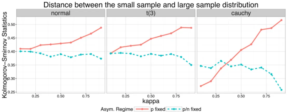
2.1 Axpproximation accuracy of p-fixed asymptotics and p/n-fixed asymptotics:

each column represents an error distribution; the x-axis represents the ra-tio  of the dimension and the sample size and the y-axis represents the Kolmogorov-Smirnov statistic; the red solid line corresponds to p-fixed

ap-proximation and the blue dashed line corresponds top/n-fixed approximation. . 14

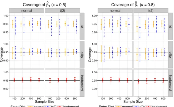
2.2 Empirical 95% coverage of ˆ₁ _with _ _{= 0}_.₅ _{(left) and} _ _{= 0}_.₈ _{(right) using} Huber1.345 loss. The x-axis corresponds to the sample size, ranging from100

to 800; the y-axis corresponds to the empirical 95% coverage. Each column represents an error distribution and each row represents a type of design. The orange solid bar corresponds to the case F = Normal; the blue dotted bar corresponds to the case F = t2; the red dashed bar represents the Hadamard

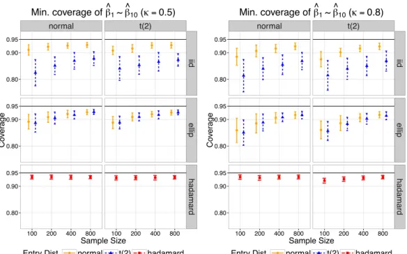
design. . . 34 2.3 Mininum empirical 95% coverage of ˆ₁ _⇠ ˆ₁₀ _with _ _{= 0}_.₅ _{(left) and} _ ₌

0.8 (right) using Huber1.345 loss. The x-axis corresponds to the sample size,

ranging from 100 to 800; the y-axis corresponds to the minimum empirical 95% coverage. Each column represents an error distribution and each row represents a type of design. The orange solid bar corresponds to the case

F = Normal; the blue dotted bar corresponds to the case F = t2; the red

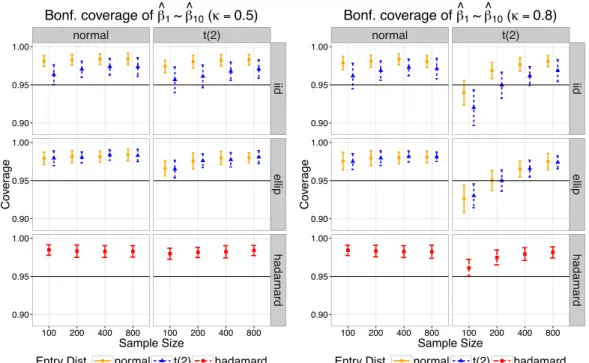
dashed bar represents the Hadamard design. . . 35 2.4 Empirical 95% coverage of ˆ₁ _⇠ ˆ₁₀ _{after Bonferroni correction with}_ _{= 0}_.₅

(left) and= 0.8(right) using Huber1.345loss. The x-axis corresponds to the

sample size, ranging from 100to800; the y-axis corresponds to the empirical uniform 95% coverage after Bonferroni correction. Each column represents an error distribution and each row represents a type of design. The orange solid bar corresponds to the caseF =Normal; the blue dotted bar corresponds to

the case F = t2; the red dashed bar represents the Hadamard design. . . 36

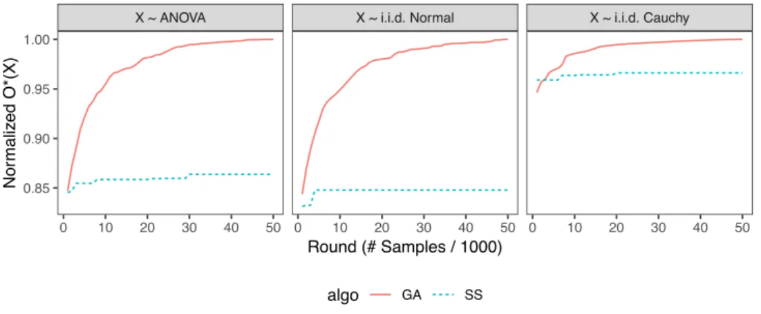
3.1 Histograms ofO⇤₍_⇧_X₎_{for a realization of a random matrix with i.i.d.}

(9)

iv 3.2 Histograms of O⇤₍_⇧_X₎ _{for three matrices as realizations of random one-way}

ANOVA matrices with exactly one entry in each row at a unifromly random position, random matrices with i.i.d. standard normal entries and random

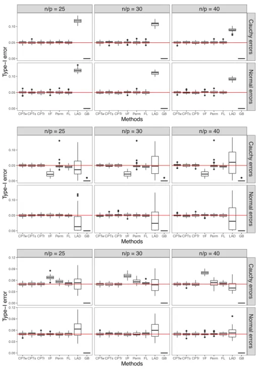
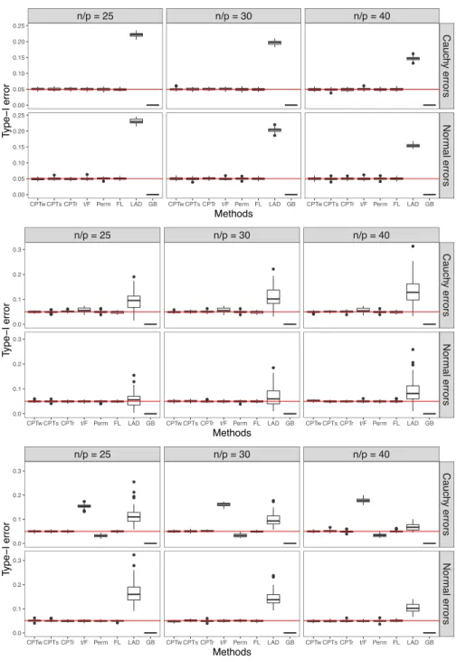
matrices with i.i.d. standard Cauchy entries, respectively. . . 50 3.3 Monte-Carlo type-I error for testing a single coordinate with three types of

X’s: (top) realizations of random matrices with i.i.d. standard normal entries;

(middle) realizations of random matrices with i.i.d. standard Cauchy entries;

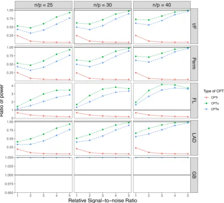
(bottom) realizations of random one-way ANOVA design matrices. . . 52 3.4 Median power ratio between each variant of CPT and each competing test for

testing a single coordinate with realizations of Gaussian matrices and Gaussian errors. The black solid line marks the equal power. The missing values in the

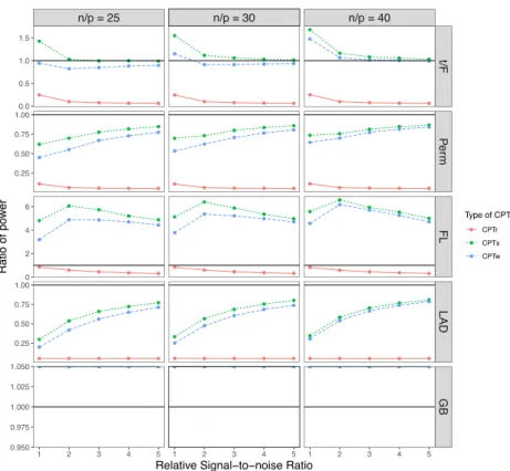
last row correspond to infinite ratios. . . 53 3.5 Median power ratio between each variant of CPT and each competing test for

testing a single coordinate with realizations of Cauchy matrices and Cauchy errors. The black solid line marks the equal power. The missing values in the

last row correspond to infinite ratios. . . 54 3.6 Monte-Carlo type-I error for testing five coordinates with three types of X’s:

(top) realizations of random matrices with i.i.d. standard normal entries; (middle) realizations of random matrices with i.i.d. standard Cauchy entries;

(bottom) realizations of random one-way ANOVA design matrices. . . 55 4.1 Simulation with ⇡1 = 0.2. X is a realization of a random matrix with i.i.d.

t(2) entries, and e(t) is a realization of a random vector with i.i.d. entries

from a distribution corresponding to each column. . . 81 4.2 Simulation. X is a realization of a random matrix with i.i.d. t(2)entries, and

e(t) is a realization of a random vector with i.i.d. entries from a distribution

corresponding to each column. . . 82 4.3 Simulation. X is a realization of a random matrix with i.i.d. t(2)entries and

e(t) is defined in (4.27): (Left)⇡1 = 0.2; (Right) ⇡1= 0.5. . . 84

4.4 Simulation. Empirical 95% coverage of t-statistics derived from the debiased

estimator with and without trimming the covariate matrix: (Left) ⇡1 = 0.2;

(Right)⇡1 = 0.5. X is a realization of a random matrix with i.i.d. t(2)entries

and e(t)is defined in (4.27). . . 85 A.1 Empirical 95% coverage of ˆ₁_with__{= 0}_.₅ _{(left) and}__{= 0}_.₈ _{(right) using}_L₁

loss. The x-axis corresponds to the sample size, ranging from 100to800; the y-axis corresponds to the empirical 95% coverage. Each column represents an error distribution and each row represents a type of design. The orange solid bar corresponds to the caseF =Normal; the blue dotted bar corresponds to

(10)

v A.2 Mininum empirical 95% coverage of ˆ₁ _⇠ ˆ₁₀ _with_ _{= 0}_.₅ _{(left) and} __{= 0}_.₈

(right) usingL1 loss. The x-axis corresponds to the sample size, ranging from

100 to800; the y-axis corresponds to the minimum empirical 95% coverage. Each column represents an error distribution and each row represents a type of design. The orange solid bar corresponds to the caseF =Normal; the blue dotted bar corresponds to the caseF = t2; the red dashed bar represents the

Hadamard design. . . 170 A.3 Empirical 95% coverage of ˆ₁ _⇠ ˆ₁₀ _{after Bonferroni correction with}_ _{= 0}_.₅

(left) and= 0.8(right) usingL1 loss. The x-axis corresponds to the sample

size, ranging from100to800; the y-axis corresponds to the empirical uniform 95% coverage after Bonferroni correction. Each column represents an error distribution and each row represents a type of design. The orange solid bar corresponds to the caseF =Normal; the blue dotted bar corresponds to the

case F = t2; the red dashed bar represents the Hadamard design. . . 171

B.1 Median power ratio between each variant of CPT and each competing test for testing a single coordinate with realizations of Gaussian matrices and Cauchy errors. The black solid line marks the equal power. The missing values in the

last row correspond to infinite ratios. . . 174 B.2 Median power ratio between each variant of CPT and each competing test for

testing a single coordinate with realizations of Cauchy matrices and Gaussian errors. The black solid line marks the equal power. The missing values in the

last row correspond to infinite ratios. . . 175 B.3 Median power ratio between each variant of CPT and each competing test

for testing a single coordinate with realizations of random one-way ANOVA matrices and Gaussian errors. The black solid line marks the equal power.

The missing values in the last row correspond to infinite ratios. . . 176 B.4 Median power ratio between each variant of CPT and each competing test

for testing a single coordinate with realizations of random one-way ANOVA matrices and Cauchy errors. The black solid line marks the equal power. The

missing values in the last row correspond to infinite ratios. . . 177 B.5 Median power ratio between each variant of CPT and each competing test for

testing five coordinates with realizations of Gaussian matrices and Gaussian errors. The black solid line marks the equal power. The missing values in the

for testing five coordinates with realizations of Gaussian matrices and Cauchy errors. The black solid line marks the equal power. The missing values in the

(11)

vi B.7 Median power ratio between each variant of CPT and each competing test

for testing five coordinates with realizations of Cauchy matrices and Gaussian errors. The black solid line marks the equal power. The missing values in the

for testing five coordinates with realizations of Cauchy matrices and Cauchy errors. The black solid line marks the equal power. The missing values in the

last row correspond to infinite ratios. . . 181 B.9 Median power ratio between each variant of CPT and each competing test for

testing five coordinates with realizations of random one-way ANOVA matrices and Gaussian errors. The black solid line marks the equal power. The missing

values in the last row correspond to infinite ratios. . . 182 B.10 Median power ratio between each variant of CPT and each competing test for

testing five coordinates with realizations of random one-way ANOVA matrices and Cauchy errors. The black solid line marks the equal power. The missing

values in the last row correspond to infinite ratios. . . 183 S1 Simulation. X is a realization of a random matrix with i.i.d. N(0,1) entries

ande(t)is a realization of a random vector with i.i.d. entries: (Left)⇡1= 0.2;

(Right) ⇡1= 0.5. Each column corresponds to a distribution ofe(t). . . 210

S2 Simulation. X is a realization of a random matrix with i.i.d. N(0,1) entries

and e(t)is defined in (4.27): (Left) ⇡1= 0.2; (Right) ⇡1= 0.5. . . 211

S3 Simulation. X is a realization of a random matrix with i.i.d. t(1)entries and

e(t) is a realization of a random vector with i.i.d. entries: (Left) ⇡1 = 0.2;

(Right) ⇡1= 0.5. Each column corresponds to a distribution ofe(t). . . 212

S4 Simulation. X is a realization of a random matrix with i.i.d. t(1)entries and

e(t) is defined in (4.27): (Left)⇡1 = 0.2; (Right) ⇡1= 0.5. . . 213

S5 Simulation on Lalonde dataset. e(t) is a realization of a random vector with

i.i.d. entries. Each column corresponds to a distribution of e(t). . . 214

S6 Simulation on Lalonde dataset. e(t) is defined in (4.27). . . 215 S7 Simulation on STAR dataset. e(t) is a realization of a random vector with

i.i.d. entries. Each column corresponds to a distribution of e(t). . . 216

(12)

vii

Acknowledgments

First and foremost, I would like to thank my terrific advisors at UC Berkeley, Professor Peter Bickel and Professor Michael Jordan, Professor Noureddine El Karoui, Professor William Fithian and Professor Peng Ding. Without their tremendous eﬀorts and patience, I would not have been able to work as an academic statistician and contact with a multitude of areas. My first formal project was supervised by Noureddine and Peter, who impressed me with their sagacity, knowledgeability and sharpness. I learned so many deep insights from the discussion between Noureddine and Peter in our regular weekly meetings for three years. During the period when I doubted if the problem could be solved, Noureddine came up with the remarkable ideas and techniques which turn out to be the key to the project. Although the final paper is 90-pages long, Noureddine checked the proof line by line and revised the paper in great details, even in the midst of his sabbatical. Had I not been advised by him, I would not have even touched a corner of the iceberg. I deeply appreciate his tremendous eﬀorts and patience as a remarkable advisor for over three years. Later on I was so fortunate to keep working with Peter on other projects beyond pure theory driven by real-world problems. Peter is the most ingenious statistician I have ever interacted with. He has numerous ideas which appear to be abstract and vague at the beginning, but always turn out to work and lead to mind-blowing methodologies. I cannot forget the exciting moments when I managed to understand the essence of Peter’s proposals, followed by a big "wow".

Being advised by Mike has been yet another stroke of great fortune. Mike is a "walking encyclopedia" with a vast knowledge across numerous disciplines, without which I could not have seen interesting results in diﬀerent areas. He has always been kind and supportive to me as well as my crazy research ideas. The acronym SCSG, coined by Mike for one of our algorithm, is perfect to describe his figure in my mind – Savvy, Creative, Supportive and Gentle. Mike also provided an extraordinary research environment, marked by his remarkable weekly group meeting. As a curiosity-driven researcher, it is of great benefit for me to read materials on diverse topics, ranging from causal inference to stochastic diﬀerential equations to mechanism designs, together with his wonderful students.

My collaboration with Will started from his fabulous course on selective inference. Being one of the five enrolled student, my questions filled in almost every one of his lecture. I was thankful that he did not kick me out of the classroom for being overly challenging and was totally impressed by the clarity of the answers and the deep insights behind. The course was so interesting and inspiring that my course project was later turned into my first conference publication. In the following collaborations, Will was never falling short of creative ideas or accurate intuition. His geometry-driven thinking patterns complements my algebra-driven perspective and greatly improves my research skills.

Peng was my role model in college and I cannot express how excited I were when he chose to join our department as an assistant professor. I must attribute all my research interests on causal inference to Peng, who taught me this long-standing topic seriously and thoroughly. Our collaborations were always smooth and eﬃcient due to his kindness and patience. Beyond his intelligence, I was greatly impressed by his wide knowledge of statistical

(13)

viii history as a junior faculty, which significantly impacted my vision and philosophy of being a statistician.

My thanks also go to other professors, in particular Professor Venkat Anantharam, who was extremely kind to be on both my qualifying exam and dissertation committees and provided helpful comments; Professor Cari Kaufman, who provided guidance and led me into the Bayesian world in my first semester at Berkeley; Professor Avi Feller, who is one of the core organizer of the weekly causal reading group which drastically influenced my research and motivated a line of joint works; Professor Jasjeet Sekhon, who provided crucial comments in our joint work; Professor Bin Yu, who taught the excellent 215A course that exemplified the charm of applied statistics an reshaped my principle of being a good statis-tian; Professor Martin Wainwright, who taught the wonderful 210B course which laid the solid theoretical foundation for my research; Professor Christopher Paciorek, who provided enormous support for softwares and computation in my research; Professor Elizaveta Levina from University of Michigan, who invited me to join the force of her project and provided instructive and insightful guidance; Professor Guido Imbens from Stanford University, who gave a thought-provoking talk at Berkeley and motivated a joint project. The thanks are also extended to Professor David Tse, Professor Stefan Wager, Professor Emmanuel Can-dès, Professor Cho-Jui Hsieh, Professor Elizaveth Levina, Professor Xuming He, Professor Yingying Fan, Professor Fredrik Sävje, Professor Kai Zhang, Professor Chaitra Nagaraja and Professor Linda Zhao for inviting me to give academic talks, which are encouraging as a junior researcher. In addition, I would like to thank my past and current collaborators Cheng Ju, Yuting Ye, Jianbo Chen, Alexander D’Amour, Aaditya Ramdas, Chiao-Yu Yang, Nhat Ho, Yuchen Wu, Tianxi Li, Sharmodeep Bhattacharyya, Purnamrita Sarkar, Melih Elibol, Samuel Horvath, Hongyuan Cao, Zitong Yang, Xingmei Lou and Xiaodong Li.

Next I would to express gratitude to our department and Ph.D. program, which I am very proud of. I am grateful to all staﬀ, especially La Shana, who is always there helping me with numerous subtle issues patiently. I am also very thankful to my excellent fellow students from whom I learn a lot from our academic discussions, in particular Eli Ben-Michael, Joseph Borja, Yuansi Chen, Billy Fang, Han Feng, Ryan Giordano, Johnny Hong, Steve Howard, Kenneth Hung, Chi Jin, Sören Künzel, Hongwei Li, Lisa Li, Xiao Li, Tianyi Lin, Sujayam Saha, Jake Soloﬀ, Sara Stoudt, Wenpin Tang, Yu Wang, Yuting Wei, Jason Wu, Siqi Wu, Zhiyi You, Da Xu, Renyuan Xu, Chelsea Zhang and Yumeng Zhang. Further I am indebted to my academic friends outside Berkeley, including but not limited to Yu Bai, Fang Cai, Xi Chen, Chao Gao, Xinzhou Guo, Zhichao Jiang, Asad Lodhia, Eugene Katsevich, Jason Lee, Song Mei, Nicole Pashley, Zhimei Ren, Feng Ruan, Weijie Su, Qingyun Sun, Pragya Sur, Jingshen Wang, Jingshu Wang, Sheng Xu, Yiqiao Zhong and Qingyuan Zhao.

Finally, I owe the most to my family. My wife Xiaoman Luo always has the magic to bring me peace and confidence when I was stressful, anxious and helpless. Her sense of humor is the major source of happiness outside my academic life. Meeting and marrying her is my greatest achievement over the past five years that is more important than any publication or academic achievement. My parents are always supportive in spite of 6500 miles between us. I could not have made any achievement without their unconditional love and support.

(14)

1

Chapter 1 Introduction

Inference from data lies at the heart of modern scientific research. Etymologically, the word "inference" means to "carry forward" and can be dated back to late 16th century from medieval Latin. Despite the solid philosophical and logical foundation, inference is never an easy task in practice due to uncertainty inherent in data. Statistics, pinoneered in 17th century and rapidly developed since early 20th century, is a discipline to generate frameworks and methodologies to understand and handle uncertainty in inference and decision making. Perhaps for this reason, statistical inference grows as a major approach of inference which is widely adopted in scientific areas.

Recent years have seen a remarkable burst of advances in data collection technology, which have created a dizzying array of exciting application areas for statistical inference. Nowadays phrases like "data science" and "big data" become the new fashion sweeping the social media. As a college student majored in statistics, I was deeply attracted by various fancy concepts and methodologies in modern statistics, marked by the development in 1990s such as sparse regression methods, statistical learning methods, social networks, etc.. But at the same time, my curiosity of classical statistics accrues as I delved further into the area. "What happened in statistics before 1990s?" – This is a question always haunting my minds. After all, the development over the past century laid the foundation for the success of modern statistics in the era of big data. Although I occasionally learned some classical topics from the textbooks, it is not even close to a complete story.

My journey to the old territory of statistics began upon reading Ronald A. Fisher’s 1922 article "On the Mathematical Foundation of Theoretical Statistics". In this pioneering work, he summarized the purpose of statistical methods as "the reduction of data" and more specifically, he wrote:

A quantity of data, which usually by its mere bulk is incapable of entering the mind, is to be replaced by relatively few quantities which shall adequately rep-resent the whole, or which, in other words, shall contain as much as possible, ideally the whole, of the relevant information contained in the original data.

(15)

CHAPTER 1. INTRODUCTION 2 an estimand and an estimator, thereby emphasizing the importance to identify the "source of randomness" in statistical inference. Furthermore, he categorized statistical problems into three

types:-(1) Problems of Specification. These arise in the choice of the mathematical form of the population.

(2) Problems of Estimation. These involve the choice of methods of calculating from a sample statistical derivates, or as we shall call them statistics, which are designed to estimate the values of the parameters of the hypothetical population. (3) Problems of Distribution. These include discussions of the distribution of statistics derived from samples, or in general any functions of quantities whose distribution is known.

Over the last century, "problems of specification" led to a plethora of statistical models (e.g. linear models, randomization models, time series models, etc.) and identification strategies; "problems of estimation" motivated the decision theoretic framework and criteria (e.g. unbiasedness, minimaxity, admissibility, etc.); "problems of distribution" generated the framework of hypothesis testing and the notion of confidence intervals, as well as the solid asymptotic distributional theory.

This remarkable categorization is still valid and quite comprehensive in modern statistics, which is equipped by advanced techniques and refined methodologies but mostly aims at handling the above three tasks. It is therefore valuable for researchers to look back on history, itself being the future of earlier history, to understand how ideas, languages, techniques and methodologies evolved, as opposed to what they appeared in textbooks written from hindsight. For instance, had I been a statistician in 1970, I would be more likely than a statistician today to be familiar with Edgeworth expansion, due to the approximation theory for t-test and F-test in absence of normality (e.g. Bartlett 1935; Wallace 1958). As a result, it would be more likely for me to understand, or even to discover, the mind-blowing connection between Edgeworth expansion and higher-order accuracy of bootstrap, developed in late 1980s (e.g. Hall 1989, 1992). Similarly, had I been familiar with the early development of design-based inference (e.g. Neyman 1923; Welch 1937; Cornfield 1944) and survey sampling (e.g. Neyman 1934; Cochran 1977), it would be easier for me to understand the modern design-based causal inference under the potential outcomes framework (e.g. Freedman 2008b,a; Lin 2013; Bloniarz et al. 2016; Abadie et al. 2017). Those who are familiar with classical statistics are more likely able to find and polish the "scattered pearls" that were under-studied or forgotten over the course of history to bring back their brilliance. On the other hand, the models and the methodologies in classical statistics may not be fully understood in spite of the long history. For instance, the linear model is over 100 years old but it still inspires new research questions in modern statistics. One remarkable example is the breakdown of classical maximum likelihood theory for linear models in moderate di-mensions, where the number of predictors grows linearly with sample size. (Bean et al. 2013) showed that the optimal M-estimator in this regime is no longer the maximum likelihood es-timator but is associated with a complicated loss function determined by a nonlinear system

(16)

CHAPTER 1. INTRODUCTION 3 that involves the design properties, the sample size per parameter as well as the error distri-bution (El Karoui et al. 2011). The astonishing finding quickly attracted further attention (e.g. El Karoui 2013, 2015; Donoho and Montanari 2015; Donoho and Montanari 2016; Sur et al. 2017; Sur and Candès 2019). Although some earlier works (e.g. Huber 1973a; Bickel and Freedman 1983a) found evidence of non-standard properties of moderate dimensional regime, the aforementioned line of work was fueled by the advances in random matrix theory and statistical physics. These works are not purely theoretical pursuit. Instead, they suggest that the standard softwares may report misleading numbers in many applications even for well-studied linear models. This is a huge warning for practitioners and will inspire further eﬀorts in the future to robustify the built-in algorithms. This inspiring example suggests the tremendous value of investigating classical statistical problems from new perspectives and equipped with advanced techniques.

In my dissertation, I will investigate three classical statistical problems but develop novel ideas and techniques to solve them, which I refer to as "modern". Of course, this is an exaggeration since three examples are far too restrictive to show the glamour of modern statistical inference. Nonetheless, they are epitomes of the elegance and the surprise when modern statistical knowledge meets classical statistical problems. In particular, all works in the dissertation deal with "problems of distribution", in which I found the classical statistics leave numerous unsolved questions while modern techniques and methodologies have great potential to come into play. I sketch the three works in each of the following subsections respectively.

1.1 Regression

M

-Estimates in Moderate Dimensions

Given a linear model y = X ⇤₊_✏_{with outcome vector} _y ₂ _Rn_{, design matrix} _X

2 Rn⇥p_,

coeﬃcient vector ⇤ ₂_Rp _{and stochastic errors}_✏

2Rn_{, an regression M-estimator is defined}

as ˆ(⇢) = arg min 2Rp n X i=1 ⇢(yi xTi ).

M-estimators were proposed by Peter J. Huber in 1960s (Huber 1964) and have been widely studied in literature (e.g. Relles 1968; Yohai 1972; Huber 1973a; Yohai and Maronna 1979a; Portnoy 1984, 1985; Mammen 1989, 1993). In a nutshell, when the sample size per parameter

n/p tends to infinity, under some regularity conditions, ˆ(⇢) is consistent in L2 metric and

is asymptotically normal in the sense that for any fixed sequence of vectors an2Rp,

aT n( ˆ(⇢) ⇤) p aT n⌃nan =₎N(0,1), where⌃= Cov( ˆ(⇢)). (1.1)

However, the story completely changes in the moderate dimensional regime, wherep/n_!

 ₂ (0,1). In moderate dimensions, the sample size per parameter is bounded away from

(17)

CHAPTER 1. INTRODUCTION 4 least-squares estimators, Huber (1973a) proved that (1.1) is impossible for every sequence of an’s in moderate dimensions. For general M-estimators with particular random designs,

El Karoui et al. (2011) showed the inconsistency of ˆ(⇢)inL2 metric and characterized the

limiting L2 risk as the solution of a delicate nonlinear system involving , the distribution

of Xand the distribution of errors. On the other hand, Bean et al. (2013) proved (1.1) with

Gaussian design matrices for any fixed sequence of an’s in moderate dimensions. This is

not contradicted to Huber (1973a) as the latter assumes a fixed design and thus the claim (1.1) only involves the randomness from ✏, while Bean et al. (2013)’s result also considers the randomness of design matrices which brings more regularity.

These works inspired a line of studies that extended the results to general settings (El Karoui 2013, 2015; Donoho and Montanari 2015; Donoho and Montanari 2016; Sur et al. 2017; Sur and Candès 2019). However, most of them focused on special random designs, such as Gaussian matrices or random matrices with elliptically distributed rows. Furthermore, their central research question is to determine the limiting risk of ˆ(⇢). Although some attempts have been made to the "problem of distribution", the results are based on Gaussian designs (Bean et al. 2013; Donoho and Montanari 2016; Sur et al. 2017; Sur and Candès 2019), with a few exceptions on more general random designs (El Karoui 2015, 2018), and some of them are about the "bulk distribution" of all coeﬃcients which is less interpretable to practitioners. No distributional result was established previously for general M-estimators with fixed designs in moderate dimensions.

In this chapter, we ask a classical question: what is the asymptotic distribution of a given coordinate of ˆ(⇢) in moderate dimensions assuming a fixed design. This question is surprisingly hard to answer than it appears to be, mainly due to the fundamental diﬃculty lying in the moderate dimensional regime. Unlike the low dimensional regime , in which the estimator has asymptotically linearity and thus the Linderberg-Feller-type central limit the-orem can be applied to prove the asymptotic normality, the Taylor-expansion-type argument does not carry over to in moderate dimensional regime because there is only bounded num-ber of samples on average for each parameter. Instead, we apply the second-order Poincaré inequality (Chatterjee 2009) that can be regarded as a generalization of classical central limit theorem to nonlinear transformation of independent random variables. In addition, we replace the Taylor-expansion-type argument by a more involved leave-one-out argument that generalizes El Karoui (2013)’s techniques to fixed-designs. In summary, we prove the following result.

Theorem 1.1.1 (Informal Version). Under appropriate conditions on the design matrixX,

the distribution of ✏ and the loss function⇢, as p/n!2(0,1), while n! 1,

max 1jpdTV 0 @_L 0 @ ˆj(⇢) j⇤ q Var( ˆj(⇢)) 1 A, N(0,1) 1 A=o(1)

(18)

CHAPTER 1. INTRODUCTION 5 We also show a counterexample, namely the one-way analysis of variance problem with non-normal errors, to emphasize that our technical assumptions are not an artifact of the proof but essential to some extent, thereby revealing the non-standard property of the mod-erate dimensional regime.

This chapter is adapted from my joint work with Professor Noureddine El Karoui and Professor Peter J. Bickel. The paper was published on Probability Theory and Related Fields on December, 2018 (Lei et al. 2018). The idea was originated from Noureddine El Karoui and Peter Bickel as an extension of their earlier works (El Karoui et al. 2011; El Karoui 2013; Bean et al. 2013; El Karoui 2015, 2018). Noureddine El Karoui and Peter Bickel provided joint advising on this work, with joint meetings of the three of us weekly over the course of two years or so.

1.2 Exact Inference for Linear Models

Chapter 2 highlights the diﬃculty in deriving asymptotics even for a single coordinate with a bounded number of samples per parameter. However, the moderate dimensional regime is quite common in practice asn/p50in many applications. This may suggest the frangibility of classical asymptotic theory which back up the numbers reported (e.g. p-values, confidence intervals) by standard softwares. It is thus natural to ask if there exists a robust inferential procedure in moderate dimensional regime.

In this chapter, we consider the problem of testing a linear hypothesis, under the linear models studied in Chapter 2, in the form H0:RT ⇤ = 0, where R 2Rp⇥r is a matrix with

full collumn rank. In particular, if R= (1,0, . . . ,0)T_{, then it is equivalent to testing for the}

first coordinate. Suppose we can find a valid test, then a confidence interval can be obtained for ⇤

1 by inverting the test, thereby yielding a valid inferential procedure, at least for a single

coordinate.

Testing linear hypotheses for linear models is a century-long problem started in 1920s and various qualitatively diﬀerent strategies have been proposed to tackle this problem, including normal theory based methods (e.g. Fisher 1922; Fisher 1924; Snedecor 1934), permutation-based methods (e.g. Pitman 1937b,a; Pitman 1938), rank-based methods (e.g. Friedman 1937; Theil 1950a), tests based on regression R-estimates (e.g. Hájek 1962), M-estimates (e.g. Huber 1973a), L-M-estimates (e.g. Bickel 1973), resampling-based methods (e.g. Freedman 1981) and other methods (e.g. Brown and Mood 1951; Daniels 1954; Hartigan 1970; Meinshausen 2015). However, as opposed to the location problems and analysis of variance problems, none of those tests are provably robust to the moderate dimensional regime under reasonably general assumptions.

In this chapter, we propose the cyclic permutation test (CPT), which is an exact non-randomized test for a given confidence level ↵, forarbitrary fixed design matrices and

arbi-trary exchangeable errors, provided that1/↵ is an integer andn/p 1/↵ 1. For instance,

CPT only requires n/p 19 when ↵ = 0.05 and thus works in moderate dimensions. No-tably, exact tests for general linear hypotheses are rare over the past century and they

(19)

CHAPTER 1. INTRODUCTION 6 are all restricted to linear models with stringent assumptions. By contrast, CPT is exact in finite samples and almost assumption-free except for the exchangeability of errors. We show that CPT has comparable power with existing tests, which may not have guarantee of validity, through extensive numerical experiments. The existence of such a non-standard, assumption-free but powerful test suggests that "problem of distribution" may be tackled by new techniques.

This chapter is adapted from my joint work with Professor Peter J. Bickel. The preprint was posted on ArXiv on July, 2019 (Lei and Bickel 2019).

1.3 Regression Adjustment for Neyman-Rubin Models

In 1923, Jerzy Neyman proposed a model for analyzing agonormic trials in his master thesis (Neyman 1923), which is later known as randomization model (Scheﬀé 1959), and quickly became one of the main pillar in analysis of experimental data (e.g. Kempthorne 1952) and survey sampling (e.g. Cochran 1977). Notably, Donald B. Rubin introduced this model into causal inference, established the framework of potential outcomes and generalized it to observational studies in his seminal work (Rubin 1974). For this reason, the randomization model is also called Neyman-Rubin model in causal inference literature.

Neyman-Rubin model is fundamentally diﬀerent from linear models. The linear model with fixed designs, marked by analysis of variance, assumes that the treatment assignment is fixed and the outcome is a random variable centered at a linear function of treatment variables. By contrast, the Neyman-Rubin model assumes that the treatment assignment is random with a known distribution and the outcome is a fixed number given the treatment values. To be concrete, given a binary treatment T with observed outcomesYobs_{, the linear}

model assumes Yobs

i =↵+ Ti+✏i where ✏i is a random variable while the Neyman-Rubin

model assumesYobs

i =Yi(1)T+Yi(0)(1 T)whereYi(1)andYi(0), called potential outcomes,

are two numbers that are either fixed or independent of the treatmentTi. Clearly, the source

of randomness is different based on two models. Inference based on linear models was usually classified as model-based inference, because it uses the functional relation between the outcome and the treatment, while inference based on Neyman-Rubin models was usually classified asdesign-based inference; see Särndal et al. (e.g. 1978) and Abadie et al. (2017). On the other hand, the inferential targets are usually different for two models. For linear models, the effect of the treatment can be easily defined as , the coefficient of the treatment variable; for Neyman-Rubin models, the effect of the treatment is usually defined as the average of individual effects, i.e. 1/nPn_i₌₁(Yi(1) Yi(0)). The former can be regarded as a special

case of the latter if we treat Yi(1) = ↵+ +✏i and Yi(0) = ↵+✏i. Inference based on

Neyman-Rubin model is more general, though at the cost of the knowledge of the treatment assignment mechanism. Nonetheless, for experimental data, it comes as a free lunch as the assignment mechanism is known by design. Therefore the Neyman-Rubin model is a robust alternative to the linear model in cases where the researcher has more knowledge of the treatment assignment mechanism than that of the functional relation between observed

(20)

CHAPTER 1. INTRODUCTION 7 outcomes and the treatment.

In many applications, baseline covariates are usually collected together with the treatment assignment (e.g. demographic information of experimental subjects). A natural approach is to run a linear regression of the observed outcome on the treatment assignment and the co-variates and estimate the effect of the treatment by the corresponding regression coefficient. The fundamental difference between two models does not prevent us from evaluating this procedure, which is clearly valid for a linear model, under the Neyman-Rubin model. How-ever, Freedman (2008b) criticized this approach, showing that it may be less efficient than the naive difference-in-means estimator which completely ignores covariates. He pointed out that the failure is driven by the different sources of randomness between linear models and Neyman-Rubin models. Interestingly, Lin (2013) proposed a simple remedy by adding the interaction terms between the treatment and the covariates into the regression and showed that this estimator is never less efficient than the difference-in-means estimator in the asymp-totic regime where the number of covariates p stays fixed while the sample sizen tends to

infinity.

Based on my experience in linear models as mentioned in the last two subsections, the asymptotics based on fixed-p regime may not be reliable. For a real problem with n= 1000 and p= 50, is the asymptotic result a plausible approximation? Bloniarz et al. (2016) took

the first in a high-dimensional setting where p >> n. However they considered a diﬀerent

estimator and assumed an approximately sparse relation between the potential outcomes and the covariates. Instead, we consider Lin (2013) in a more classical setting where no assumption is imposed on the potential outcomes except some regularity conditions involving the finite sample moments. Specifically, for completely randomized experiments, we show that Lin (2013)’s estimator is consistent when logp_!0 and asymptotically normal when p _! 0 under mild moment conditions, where  is the maximum leverage score of the covariate matrix. In the favorable case where leverage scores are all close together, his estimator is consistent whenp=o(n/logn) and is asymptotically normal whenp=o(n1/2_).

Beyond this regime, we find that the estimator may have a non-negligible bias. For this reason, we propose a bias-corrected estimator that is consistent when logp _! 0 and is asymptotically normal, with the same variance in the fixed-p regime, when 2_p_log_p

! 0. In the favorable case, the latter condition reduces to p = o(n2/3_/_(log_n₎1/3_{). Our analyses}

require novel concentration inequalities for sampling without replacement, driven by modern probability theory.

This chapter is adapted from my joint work with Professor Peng Ding. The preprint was posted on ArXiv on June, 2018 (Lei and Ding 2018).

(21)

8

Chapter 2 Regression

M

-Estimates in Moderate

Dimensions

2.1 Introduction

High-dimensional statistics has a long history (Huber 1973a; Wachter 1976, 1978) with considerable renewed interest over the last two decades. In many applications, the researcher collects data which can be represented as a matrix, called a design matrix and denoted by

X ₂ Rn⇥p_{, as well as a response vector} _y

2 Rn _{and aims to study the connection between}

X and y. The linear model is among the most popular models as a starting point of data

analysis in various fields. A linear model assumes that

y =X ⇤+✏, (2.1)

where ⇤ ₂ _Rp _{is the coeﬃcient vector which measures the marginal contribution of each}

predictor and ✏is a random vector which captures the unobserved errors.

The aim of this chapter is to provide valid inferential results for features of ⇤_{. For}

example, a researcher might be interested in testing whether a given predictor has a negligible eﬀect on the response, or equivalently whether ⇤

j = 0for somej. Similarly, linear contrasts

of ⇤ _{such as} ⇤

1 2⇤ might be of interest in the case of the group comparison problem in

which the first two predictors represent the same feature but are collected from two diﬀerent groups. An M-estimator, defined as ˆ(⇢) = arg min 2Rp 1 n n X i=1 ⇢(yi xTi ) (2.2)

where ⇢ denotes a loss function, is among the most popular estimators used in practice (Relles 1968; Huber 1973a). In particular, if ⇢(x) = 1

2x

2_, _ˆ(⇢) _{is the famous Least Square}

Estimator (LSE). We intend to explore the distribution of ˆ(⇢), based on which we can achieve the inferential goals mentioned above.

(22)

CHAPTER 2. REGRESSION M-ESTIMATES IN MODERATE DIMENSIONS 9

The most well-studied approach is the asymptotic analysis, which assumes that the scale of the problem grows to infinity and use the limiting result as an approximation. In regression problems, the scale parameter of a problem is the sample sizenand the number of predictors p. The classical approach is to fixp and let n grow to infinity. It has been shown (Relles

1968; Yohai 1972; Huber 1972; Huber 1973a) that ˆ(⇢)is consistent in terms ofL2norm and

asymptotically normal in this regime. The asymptotic variance can be then approximated by the bootstrap (Bickel and Freedman 1981). Later on, the studies are extended to the regime in which both n and p grow to infinity butp/n converges to0 (Yohai and Maronna 1979b; Portnoy 1984, 1985, 1986, 1987; Mammen 1989). The consistency, in terms of theL2

norm, the asymptotic normality and the validity of the bootstrap still hold in this regime. Based on these results, we can construct a 95% confidence interval for 0j simply as ˆj(⇢)±

1.96

q d

Var( ˆj(⇢)) where Var( ˆd j(⇢)) is calculated by bootstrap. Similarly we can calculate

p-values for the hypothesis testing procedure.

We ask whether the inferential results developed under the low-dimensional assumptions and the software built on top of them can be relied on for moderate and high-dimensional analysis? Concretely, if in a study n = 50 and p = 40, can the software built upon the

assumption that p/n _' 0 be relied on when p/n = .8? Results in random matrix theory

(Marčenko and Pastur 1967) already oﬀer an answer in the negative side for many PCA-related questions in multivariate statistics. The case of regression is more subtle: For instance for least-squares, standard degrees of freedom adjustments eﬀectively take care of many dimensionality-related problems. But this nice property does not extend to more general regression M-estimates.

Once these questions are raised, it becomes very natural to analyze the behavior and performance of statistical methods in the regime where p/n is fixed. Indeed, it will help us

to keep track of the inherent statistical diﬃculty of the problem when assessing the variability of our estimates. In other words, we assume in this chapter that p/n _!  > 0 while let

n grows to infinity. Due to identifiability issues, it is impossible to make inference on ⇤

if p > n without further structural or distributional assumptions. We discuss this point in

details in Section 2.2.3. Thus we consider the regime where p/n _!  ₂ (0,1). We call it

the moderate p/n regime. This regime is also the natural regime in random matrix theory

(Marčenko and Pastur 1967; Wachter 1978; Johnstone 2001; Bai and Silverstein 2010). It has been shown that the asymptotic results derived in this regime sometimes provide an extremely accurate approximation to finite sample distributions of estimators at least in certain cases (Johnstone 2001) where nand pare both small.

2.1.1 Qualitatively Di

ﬀ

erent Behavior of Moderate

p/n

Regime

First, ˆ(⇢) is no longer consistent in terms of L2 norm and the risk Ekˆ(⇢) ⇤k2 tends

to a non-vanishing quantity determined by , the loss function ⇢ and the error distribution through a complicated system of non-linear equations (El Karoui et al. 2011; El Karoui 2013, 2015; Bean et al. 2012). This L2-inconsistency prohibits the use of standard

(23)

perturbation-CHAPTER 2. REGRESSION M-ESTIMATES IN MODERATE DIMENSIONS 10

analytic techniques to assess the behavior of the estimator. It also leads to qualitatively dif-ferent behaviors for the residuals in moderate dimensions; in contrast to the low-dimensional case, they cannot be relied on to give accurate information about the distribution of the errors. However, this seemingly negative result does not exclude the possibility of inference since ˆ(⇢) is still consistent in terms of L2+⌫ norms for any ⌫ > 0 and in particular in L1

norm. Thus, we can at least hope to perform inference on each coordinate.

Second, classical optimality results do not hold in this regime. In the regime p/n _!0,

the maximum likelihood estimator is shown to be optimal (Huber 1964; Huber 1972; Bickel and Doksum 2015). In other words, if the error distribution is known then the M-estimator associated with the loss ⇢(·) = logf✏(·) is asymptotically eﬃcient, provided the design is of appropriate type, where f✏(·) is the density of entries of ✏. However, in the moderatep/n

regime, it has been shown that the optimal loss is no longer the log-likehood but an other function with a complicated but explicit form (Bean et al. 2013), at least for certain designs. The suboptimality of maximum likelihood estimators suggests that classical techniques fail to provide valid intuition in the moderate p/n regime.

Third, the joint asymptotic normality of ˆ(⇢), as a p-dimensional random vector, may

be violated for a fixed design matrix X. This has been proved for least-squares by Huber

(1973a) in his pioneering work. For general M-estimators, this negative result is a simple consequence of the results of El Karoui et al. (2011): They exhibit an ANOVA design (see below) where even marginal fluctuations are not Gaussian. By contrast, for random design, they show that ˆ(⇢) is jointly asymptotically normal when the design matrix is elliptical with general covariance by using the non-asymptotic stochastic representation for ˆ(⇢) as well as elementary properties of vectors uniformly distributed on the uniform sphere in Rp_;

See section 2.2.3 of El Karoui et al. (2011) or the supplementary material of Bean et al. (2013) for details. This does not contradict Huber (1973a)’s negative result in that it takes the randomness from bothX and✏into account while Huber (1973a)’s result only takes the randomness from✏into account. Later, El Karoui (2015) shows that each coordinate of ˆ(⇢) is asymptotically normal for a broader class of random designs. This is also an elementary consequence of the analysis in El Karoui (2013). However, to the best of our knowledge, beyond the ANOVA situation mentioned above, there are no distributional results for fixed design matrices. This is the topic of this chapter.

Last but not least, bootstrap inference fails in this moderate-dimensional regime. This has been shown by Bickel and Freedman (1983b) for least-squares and residual bootstrap in their influential work. Recently, El Karoui and Purdom (2015) studied the results to general M-estimators and showed that all commonly used bootstrapping schemes, including pairs-bootstrap, residual bootstrap and jackknife, fail to provide a consistent variance estimator and hence valid inferential statements. These latter results even apply to the marginal distributions of the coordinates of ˆ(⇢). Moreover, there is no simple, design independent, modification to achieve consistency (El Karoui and Purdom 2015).

(24)

2.1.2 Our Contributions

In summary, the behavior of the estimators we consider in this chapter is completely diﬀerent in the moderatep/nregime from its counterpart in the low-dimensional regime. As discussed

in the next section, moving one step further in the moderate p/n regime is interesting

from both the practical and theoretical perspectives. Our main contribution is to establish coordinate-wise asymptotic normality of ˆ(⇢) for certain fixed design matrices X in this

regime under technical assumptions. The following theorem informally states our main result.

Theorem 2.1.1 (Informal Version of Theorem 2.3.1 in Section 2.3). Under appropriate

conditions on the design matrix X, the distribution of ✏ and the loss function ⇢, as p/n!

₂(0,1), whilen_{! 1}, max 1jpdTV 0 @_L 0 @ˆj(⇢) Eˆj(⇢) q Var( ˆj(⇢)) 1 A, N(0,1) 1 A=o(1)

where dTV(·,·) is the total variation distance and L(·) denotes the law.

It is worth mentioning that the above result can be extended to finite dimensional linear contrasts of ˆ_{. For instance, one might be interested in making inference on} ⇤

1 2⇤ in the

problems involving the group comparison. The above result can be extended to give the asymptotic normality of ˆ₁ ˆ₂_.

Besides the main result, we have several other contributions. First, we use a new approach to establish asymptotic normality. Our main technique is based on the second-order Poincaré inequality (SOPI), developed by Chatterjee (2009) to derive, among many other results, the fluctuation behavior of linear spectral statistics of random matrices. In contrast to classical approaches such as the Lindeberg-Feller central limit theorem, the second-order Poincaré inequality is capable of dealing with nonlinear and potentially implicit functions of independent random variables. Moreover, we use diﬀerent expansions for ˆ(⇢) and residuals based on double leave-one-out ideas introduced in El Karoui et al. (2011), in contrast to the classical perturbation-analytic expansions. See aforementioned paper and follow-ups. An informal interpretation of the results of Chatterjee (2009) is that if the Hessian of the nonlinear function of random variables under consideration is suﬃciently small, this function acts almost linearly and hence a standard central limit theorem holds.

Second, to the best of our knowledge this is the first inferential result for fixed (non ANOVA-like) design in the moderate p/nregime. Fixed designs arise naturally from an

ex-perimental design or a conditional inference perspective. That is, inference is ideally carried out without assuming randomness in predictors; see Section 2.2.2 for more details. We clarify the regularity conditions for coordinate-wise asymptotic normality of ˆ(⇢) explicitly, which are checkable for LSE and also checkable for general M-estimators if the error distribution is known. We also prove that these conditions are satisfied with by a broad class of designs.

(25)

The ANOVA-like design described in Section 2.3.3 exhibits a situation where the distri-bution of ˆ_j_(⇢) _{is not going to be asymptotically normal. As such the results of Theorem} 2.3.1 below are somewhat surprising.

For complete inference, we need both the asymptotic normality and the asymptotic bias and variance. Under suitable symmetry conditions on the loss function and the error dis-tribution, it can be shown that ˆ(⇢) is unbiased (see Section 2.3.2 for details) and thus it is left to derive the asymptotic variance. As discussed at the end of Section 2.1.1, classical approaches, e.g. bootstrap, fail in this regime. For least-squares, classical results continue to hold and we discuss it in section 2.5 for the sake of completeness. However, for M-estimators, there is no closed-form result. We briefly touch upon the variance estimation in Section 2.3.4. The derivation for general situations is beyond the scope of this chapter and left to the future research.

2.1.3 Outline

The rest of the chapter is organized as follows: In Section 2.2, we clarify details which are mentioned in the current section. In Section 2.3, we state the main result (Theorem 2.3.1) formally and explain the technical assumptions. Then we show several examples of random designs which satisfy the assumptions with high probability. In Section 4, we introduce our main technical tool, second-order Poincaré inequality (Chatterjee 2009), and apply it on M-estimators as the first step to prove Theorem 2.3.1. Since the rest of the proof of Theorem 2.3.1 is complicated and lengthy, we illustrate the main ideas in Appendix A.1. The rigorous proof is left to Appendix A.2. In Section 2.5, we provide reminders about the theory of least-squares estimation for the sake of completeness, by taking advantage of its explicit form. In Section 2.6, we display the numerical results. The proof of other results are stated in Appendix A.3 and more numerical experiments are presented in Appendix A.4.

2.2 More Details on Background

2.2.1 Moderate

p/n

Regime: a more informative type of

asymptotics?

In Section 2.1, we mentioned that the ratiop/nmeasures the diﬃculty of statistical inference.

The moderate p/n regime provides an approximation of finite sample properties with the

diﬃculties fixed at the same level as the original problem. Intuitively, this regime should capture more variation in finite sample problems and provide a more accurate approximation. We will illustrate this via simulation.

Consider a study involving 50 participants and40variables; we can either use the asymp-totics in whichpis fixed to be40,ngrows to infinity orp/nis fixed to be0.8, andngrows to

infinity to perform approximate inference. Current software rely on low-dimensional asymp-totics for inferential tasks, but there is no evidence that they yield more accurate inferential

(26)

statements than the ones we would have obtained using moderate dimensional asymptotics. In fact, numerical evidence (Johnstone 2001; El Karoui et al. 2013; Bean et al. 2013) show that the reverse is true.

We exhibit a further numerical simulation showing that. Consider a case that n= 50, ✏ has i.i.d. entries and X is one realization of a matrix generated with i.i.d. gaussian (mean

0, variance 1) entries. For  2 {0.1,0.2, . . . ,0.9} and diﬀerent error distributions, we use the Kolmogorov-Smirnov (KS) statistics to quantify the distance between the finite sample distribution and two types of asymptotic approximation of the distribution of ˆ₁_(⇢).

Specifically, we use the Huber loss function ⇢Huber,k with default parameter k = 1.345

(Huber 1981), i.e. ⇢Huber,k(x) = ⇢ 1 2x 2 |x_|_k k(|x| 1 2k) |x|> k

Specifically, we generate three design matrices X(0)_, _X(1) _and _X(2)_: _X(0) _{for small sample}

case with a sample sizen= 50and a dimensionp=n;X(1)_{for low-dimensional asymptotics}

(p fixed) with a sample size n = 1000 and a dimension p = 50; and X(2) _for

moderate-dimensional asymptotics (p/n fixed) with a sample size n= 1000and a dimension p =n.

Each of them is generated as one realization of an i.i.d. standard gaussian design and then treated as fixed acrossK = 100repetitions. For each design matrix, vectors✏of appropriate length are generated with i.i.d. entries. The entry has either a standard normal distribution, or at3-distribution, or a standard Cauchy distribution, i.e. t1. Then we use✏as the response,

or equivalently assume ⇤ _{= 0, and obtain the M-estimators} ˆ(0)_,ˆ(1)_,ˆ(2)_{. Repeating this}

procedure for K = 100 times results in K replications in three cases. Then we extract

the first coordinate of each estimator, denoted by {ˆ(0)k,1}Kk=1,{ˆ (1)

k,1}Kk=1,{ˆ (2)

k,1}Kk=1. Then the

two-sample Kolmogorov-Smirnov statistics can be obtained by KS1= r n 2 maxx | ˆ Fn(0)(x) Fˆn(1)(x)|, KS2= r n 2 maxx | ˆ Fn(0)(x) Fˆn(2)(x)|, where _Fˆ(r)

n is the empirical distribution of {ˆ_k,(r₁)}K_k₌₁. We can then compare the accuracy

of two asymptotic regimes by comparing KS1 and KS2. The smaller the value of KSi, the

better the approximation.

Figure 2.1 displays the results for these error distributions. We see that for gaussian errors and even t3 errors, the p/n-fixed/moderate-dimensional approximation is uniformly

more accurate than the widely used p-fixed/low-dimensional approximation. For Cauchy

errors, the low-dimensional approximation performs better than the moderate-dimensional one when p/nis small but worsens when the ratio is large especially when p/nis close to 1.

Moreover, when p/n grows, the two approximations have qualitatively diﬀerent behaviors:

thep-fixed approximation becomes less and less accurate while thep/n-fixed approximation

does not suﬀer much deterioration whenp/ngrows. The qualitative and quantitative

diﬀer-ences of these two approximations reveal the practical importance of exploring the p/n-fixed

(27)

CHAPTER 2. REGRESSION M-ESTIMATES IN MODERATE DIMENSIONS 14 normal t(3) cauchy ● ● ● ● ● ● ● ● ● ● ● ● ● ● ● ● ● ● ● ● ● ● ● ● ● ● ● ● ● ● ● ● ● ● _● ● ● ● ● ● ● ● ● ● ● ● ● ● ● ● ● ● ● ● 0.25 0.30 0.35 0.40 0.45 0.50 0.25 0.50 0.75 0.25 0.50 0.75 0.25 0.50 0.75 kappa K olmogoro v − Smir no v Statistics

Asym. Regime ● _{p fixed} ● _{p/n fixed}

Distance between the small sample and large sample distribution

Figure 2.1: Axpproximation accuracy ofp-fixed asymptotics andp/n-fixed asymptotics: each

column represents an error distribution; the x-axis represents the ratio  of the dimension and the sample size and the y-axis represents the Kolmogorov-Smirnov statistic; the red solid line corresponds to p-fixed approximation and the blue dashed line corresponds top/n-fixed

approximation.

2.2.2 Random vs fixed design?

As discussed in Section 2.1.1, assuming a fixed design or a random design could lead to qualitatively diﬀerent inferential results.

In the random design setting,Xis considered as being generated from a super population.

For example, the rows of X can be regarded as an i.i.d. sample from a distribution known,

or partially known, to the researcher. In situations where one uses techniques such as cross-validation (Stone 1974), pairs bootstrap in regression (Efron and Efron 1982) or sample splitting (Wasserman and Roeder 2009), the researcher eﬀectively assumes exchangeability of the data (xT

i, yi)ni=1. Naturally, this is only compatible with an assumption of random

design. Given the extremely widespread use of these techniques in contemporary machine learning and statistics, one could argue that the random design setting is the one under which most of modern statistics is carried out, especially for prediction problems. Furthermore, working under a random design assumption forces the researcher to take into account two sources of randomness as opposed to only one in the fixed design case. Hence working under a random design assumption should yield conservative confidence intervals for ⇤

j.

In other words, in settings where the researcher collects data without control over the values of the predictors, the random design assumption is arguably the more natural one of the two.

However, it has now been understood for almost a decade that common random design assumptions in high-dimension (e.g. xi = ⌃1/2zi where zi,j’s are i.i.d with mean 0 and

variance 1 and a few moments and ⌃ “well behaved") suﬀer from considerable geometric limitations, which have substantial impacts on the performance of the estimators considered

(28)

in this chapter (El Karoui et al. 2011). As such, confidence statements derived from that kind of analysis can be relied on only after performing a few graphical tests on the data (see El Karoui (2010)). These geometric limitations are simple consequences of the concentration of measure phenomenon (Ledoux 2001).

On the other hand, in the fixed design setting, X is considered a fixed matrix. In this

case, the inference only takes the randomness of ✏ into consideration. This perspective is popular in several situations. The first one is the experimental design. The goal is to study the eﬀect of a set of factors, which can be controlled by the experimenter, on the response. In contrast to the observational study, the experimenter can design the experimental condition ahead of time based on the inference target. For instance, a one-way ANOVA design encodes the covariates into binary variables (see Section 2.3.3 for details) and it is fixed prior to the experiment. Other examples include two-way ANOVA designs, factorial designs, Latin-square designs, etc. (Scheﬀe 1999).

Another situation which is concerned with fixed design is the survey sampling where the inference is carried out conditioning on the data (Cochran 1977). Generally, in order to avoid unrealistic assumptions, making inference conditioning on the design matrix X

is necessary. Suppose the linear model (2.1) is true and identifiable (see Section 2.2.3 for details), then all information of ⇤ _{is contained in the conditional distribution} _L₍_y_|_X₎ _and

hence the information in the marginal distribution L(X) is redundant. The conditional inference framework is more robust to the data generating procedure due to the irrelevance of L(X).

Also, results based on fixed design assumptions may be preferable from a theoretical point of view in the sense that they could potentially be used to establish corresponding results for certain classes of random designs. Specifically, given a marginal distribution L(X), one

only has to prove that X satisfies the assumptions for fixed design with high probability.

In conclusion, fixed and random design assumptions play complementary roles in moder-ate dimensional settings. We focus on the least understood of the two, the fixed design case, in this chapter.

2.2.3 Modeling and Identification of Parameters

The problem of identifiability is especially important in the fixed design case. Define ⇤_(⇢)

in the population as ⇤_{(⇢) = arg min} 2Rp 1 n n X i=1 E⇢(yi xTi ). (2.3)

One may ask whether ⇤_{(⇢) =} ⇤ _{regardless of} _⇢ _{in the fixed design case. We provide}

an aﬃrmative answer in the following proposition by assuming that ✏i has a symmetric

(29)

Proposition 2.2.1. Suppose X has a full column rank and ✏i d

= ✏i for all i. Further

assume ⇢ is an even convex function such that for any i= 1,2, . . . and↵ ₆= 0,

1

2(E⇢(✏i ↵) +E⇢(✏i+↵))>E⇢(✏i). (2.4)

Then ⇤_{(⇢) =} ⇤ _{regardless of the choice of} _⇢_.

The proof is left to Appendix A.3. It is worth mentioning that Proposition 2.2.1 only requires the marginals of ✏ to be symmetric but does not impose any constraint on the dependence structure of ✏. Further, if ⇢ is strongly convex, then for all↵ 6= 0,

1

2(⇢(x ↵) +⇢(x+↵))>⇢(x).

As a consequence, the condition (2.4) is satisfied provided that ✏i is non-zero with positive

probability.

If ✏ is asymmetric, we may still be able to identify ⇤ if ✏i are i.i.d. random variables.

In contrast to the last case, we should incorporate an intercept term as a shift towards the centroid of ⇢. More precisely, we define↵⇤_(⇢) _and ⇤_(⇢) _as

(↵⇤(⇢), ⇤(⇢)) = arg min ↵2R, 2Rp 1 n n X i=1 E⇢(yi ↵ xTi ).

Proposition 2.2.2. Suppose(1, X) is of full column rank and✏i are i.i.d. such thatE⇢(✏1

↵) as a function of ↵ has a unique minimizer ↵(⇢). Then ⇤_(⇢) _{is uniquely defined with}

⇤_{(⇢) =} ⇤ _and _↵⇤_{(⇢) =}_↵(⇢)_.

The proof is left to Appendix A.3. For example, let ⇢(z) = _|z_|. Then the minimizer of

E⇢(✏1 a) is a median of ✏1, and is unique if✏1 has a positive density. It is worth pointing

out that incorporating an intercept term is essential for identifying ⇤_{. For instance, in the}

least-square case, ⇤_(⇢) _{no longer equals to} ⇤ _if _E_✏

i 6= 0. Proposition 2.2.2 entails that

the intercept term guarantees ⇤_{(⇢) =} ⇤_{, although the intercept term itself depends on the}

choice of ⇢unless more conditions are imposed.

If ✏i’s are neither symmetric nor i.i.d., then ⇤ cannot be identified by the previous

criteria because ⇤_(⇢)_{depends on}_{⇢. Nonetheless, from a modeling perspective, it is popular}

and reasonable to assume that ✏i’s are symmetric or i.i.d. in many situations. Therefore,

Proposition 2.2.1 and Proposition 2.2.2 justify the use of estimators in those cases and M-estimators derived from diﬀerent loss functions can be compared because they are estimating the same parameter.