Application of Machine Learning Techniques to Delay Tolerant Network Routing

APPLICATION OF MACHINE LEARNING TECHNIQUES TO

DELAY TOLERANT NETWORK ROUTING

by

RACHEL DUDUKOVICH

Submitted in partial fulfillment of the requirements

For the degree of Doctor of Philosophy

Thesis Adviser: Dr. Christos Papachristou

Electrical Engineering and Computer Science CASE WESTERN RESERVE UNIVERSITY

Network Routing

Case Western Reserve University

Case School of Graduate Studies

We hereby approve the thesis1of

RACHEL DUDUKOVICH

for the degree of

Doctor of Philosophy

December 5, 2018

Dr. Christos Papachristou

Committee Chair, Adviser Date

Department of Electrical, Computer, and Systems Engineering

Dr. Pan Li

Committee Member Date

Department of Electrical, Computer, and Systems Engineering

Dr. Ming-Chun Huang

Committee Member Date

Department of Electrical, Computer, and Systems Engineering

Dr. An Wang

Committee Member Date

Department of Computer Science

1_{We certify that written approval has been obtained for any proprietary material contained} therein.

Department of Computer Science

Dr. Daniel Saab

Committee Member Date

Department of Electrical, Computer, and Systems Engineering

Dr. Francis Merat

Committee Member Date

Department of Electrical, Computer, and Systems Engineering

Dr. Daniel Raible

Committee Member Date

NASA GRC

Alan Hylton

Committee Member Date

NASA GRC

List of Tables vi

List of Figures vii

List of Acronyms xi

Acknowledgements xiv

Abstract xv

Chapter 1. Introduction 1

Objective and Description 1

Motivation 3

Contributions 5

Outline 6

Chapter 2. Background 8

NASA SCaN Networks 8

Delay Tolerant Networking 10

Machine Learning 26

Chapter 3. Related Work 38

DTN Routing Algorithms 38

Machine Learning Based DTN Routing Algorithms 50

Chapter 4. Approach 52

Architecture 52

Q-Routing 56

Classification Based Routing 61

Chapter 5. Implementation 70

DTN Implementations 71

Machine Learning Routing Implementation 74

IBR-DTN Modifications 76

Learning Procedures 83

Machine Learning Libraries 93

Chapter 6. Simulation and Emulation 95

Simulation Environment 96

Emulation Environment 100

Scenarios 107

Tool Chain and Automation 112

Chapter 7. Performance Measurements 118

Metrics 119

Survey of DTN Routing Performance 126

Q-Routing Simulation Results 131

Multi-label Classification Approach 140

Clustering Results 151 Chapter 8. Conclusions 158 Summary 158 Conclusion 159 Future Work 160 References 162 v

2.1 Approximate Round Trip Times of Network Assets [1] 10

3.1 Summary of DTN Routing Algorithms 40

3.2 RAPID Routing Metrics 44

4.1 Algorithm Summary 56

7.1 Confusion Matrix 123

7.2 DTNBone Availability Schedule 127

7.3 Results for 50 1 KB Bundles 128

7.4 Network Configuration for Simulation 1 132

7.5 Network Configuration for Simulation 2 134

7.6 Nodes Selected for Failure 135

7.7 Network Configuration for Simulation 5 138

7.8 Cluster Metrics for Number of Clusters 152

2.1 Example Mission Operations Center to Deep Space Rover

Protocol Stack[2] 12

2.2 DTN Top Level Flow Chart 15

2.3 Bundle Protocol Primary Block 17

2.4 Bundle Protocol Payload Block 17

2.5 Bundle Protocol Transmission Procedure 18

2.6 Bundle Protocol Reception Procedure 22

2.7 Discovery Beacon Format 24

2.8 Reinforcement Learning Example 27

2.9 Decision Tree Illustration 32

2.10 K-Nearest Neighbors Illustration 34

3.1 CGR Contact Review Procedure 48

3.2 CGR Forwarding Decision 49

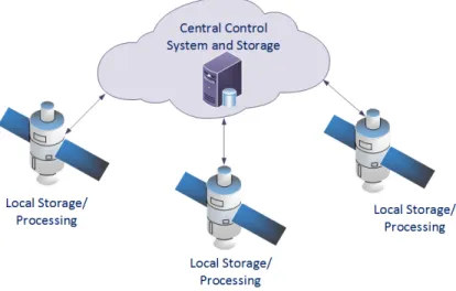
4.1 Centralized Learning Architecture 53

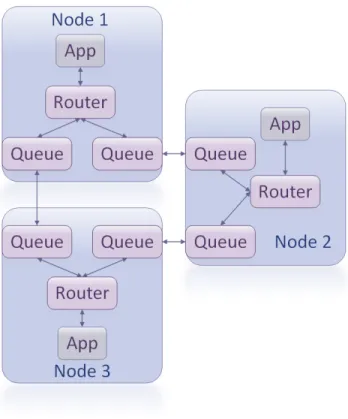
4.2 Distributed Learning Architecture 54

4.3 Q-Routing Simulation Modules 59

4.4 Example Node and Q-Table 60

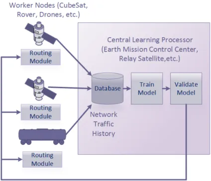
4.5 High Level Learning Architecture 65

4.6 Example Classifier Attribute Vector and Prediction 65

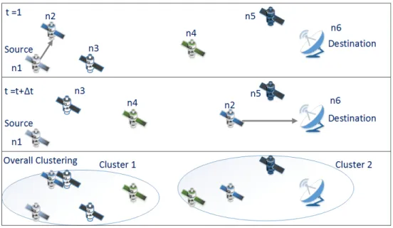
4.7 Example of Clustering Over Time with K=2 67

4.8 Clustering Block Diagram 68

5.3 IBR-DTN Base Router 78

5.4 IBR-DTN Neighborhood Routing Extension 80

5.5 Classification Routing Extension 82

6.1 OMNeT++ Simulation Environment 97

6.2 The ONE Simulation Environment 99

6.3 CORE Screen Shot 102

6.4 CORE/EMANE Architecture 106

6.5 STK Analysis for ISS Scenario 108

6.6 STK Access Times for ISS Scenario 109

6.7 ISS Scenario in CORE 110

6.8 ISS Scenario in sdt3d 110

6.9 Emulation Tool Chain 113

7.1 Network Topology of the NASA DTNBone 127

7.2 Average Delay for 2 Hop Path 129

7.3 Average Delay 10 Node Mesh 133

7.4 Average Delay for 20 Node Mesh 135

7.5 Average Delay Versus Number of Nodes Failing 136

7.6 Average Delay with Forgetting Policy 137

7.7 Average End-to-End Delay Based on Propagation Delay 139 7.8 Average End-to-End Delay Versus Data Rate 139

7.11 Jaccard Similarity Score (Random Walk) 143

7.12 Jaccard Similarity Score (ZebraNet) 143

7.13 Hamming Loss (Random Walk) 144

7.14 Hamming Loss (ZebraNet) 144

7.15 Zero-One Loss (Random Walk) 145

7.16 Zero-One Loss (ZebraNet) 145

7.17 Epidemic versus Classification Filter TCP CL Bytes Transmitted 146 7.18 Epidemic versus Classification Filter TCP CL Bytes Received 147 7.19 Epidemic versus Classification Filter Bundle Delivery Ratio 148 7.20 Epidemic versus Classification Filter Bundle Delivery Cost 148 7.21 Epidemic versus Classification Bundles Replicated 149 7.22 Epidemic versus Classification Bundles Expired 149 7.23 Epidemic versus Classification Bundles Queued 150 7.24 Epidemic versus Classification Bundle Delivery Delay 151 7.25 Graphical Representation of Location Clusters 152 7.26 Epidemic versus Cluster Filter TCP CL Bytes Transmitted 153 7.27 Epidemic versus Cluster Filter TCP CL Bytes Received 154 7.28 Epidemic versus Cluster Filter Bundle Delivery Ratio 154 7.29 Epidemic versus Cluster Filter Bundle Delivery Cost 155 7.30 Epidemic versus Cluster Bundles Replicated 155

7.33 Epidemic versus Cluster Bundle Delivery Delay 157

API: Application Program Interface

BP: Bundle Protocol

BR: Binary Relevance

CC: Classifier Chain

CCSDS: Consultative Committee for Space Data Systems

CFDP: CCSDS File Delivery Protocol

CGR: Contact Graph Routing

CL: Convergence Layer

CORE: Common Open Research Emulator

CRAWDAD: Community Resource for Archiving Wireless Data At Dartmouth

DHCP: Dynamic Host Configuration Protocol

DSN: Deep Space Network

DTLSR: Delay Tolerant Link State Routing

DTN: Delay Tolerant Network

ECC: Ensemble of Classifier Chains

EID: Endpoint Identifier

EMANE: Extendable Mobile Ad-hoc Network Emulator

ETO-CGR: Earliest Transmission Opportunity Contact Graph Routing

FTP: File Transfer Protocol

GIL: Global Interpreter Lock

GPS: Global Positioning System

HBSD: History Based Scheduling and Drop

HTTP: HyperText Transfer Protocol

ID3: Iterative Dichotomiser 3

ION: Interplanetary Overlay Network

IP: Internet Protocol

IPND: IP Neighbor Discovery

JNI: Java Native Interface

LATA: Local Access and Transport Area

LEO: Low Earth Orbit

LoWPAN: Low-Power Wireless Personal Area Networks

LTP: Licklider Transmission Protocol

LXC: Linux Container

MAC: Media Access Control

MANET: Mobile Ad-Hoc Network

MAP: Maximum A Posteriori

MSB: Most Significant Bit

NBF: Neighborhood Bloom Filter

NED: Network Description

NEM: Network Emulation Module

NEN: Near Earth Network

NORM: NACK-Oriented Reliable Multicast

NS-2: Network Simulator 2

OLSR: Optimized Link State Routing

ONE: Opportunistic Network Environment

OSI: Open Systems Interconnection

Pandas: Python Data Analysis

PCN: Planetary Communication Network

POSIX: Portable Operating System Interface

PRoPHET: Probabilistic Routing Protocol using History of Encounters and Tran-sitivity

RAPID: Resource Allocation Protocol for Intentional DTN

RSA: Rivest-Shamir-Adleman

RTEMS: Real-Time Executive for Multiprocessor Systems

SCaN: Space Communications and Navigation

SDNV: Self-Delimiting Numeric Values

SDT3D: Scripted Display Tools 3D

SN: Space Network

SSH: Secure Socket Shell

SSL: Secure Sockets Layer

STK: Systems Tool Kit

TD: Temporal Difference

TDRS: Tracking Data Relay Satellite

UDP: User Datagram Protocol

URI: Uniform Resource Identifier

UTM: Universal Transverse Mercator

VANET: Vehicular Ad-Hoc Network

XML: eXtensible Markup Language

:

I would like to express my gratitude to my advisor, Dr. Christos Papachristou for his guidance and support over several years of having been his student. I would like to thank the members of the HiDRA team at NASA Glenn Research Center for their help and support, especially Dr. Daniel Raible, Alan Hylton, Gilbert Clark, Tom Kacpura and Gary Pease, and Dennis Iannicca for help with DTNbone testing and paper reviews. In addition, I would like to thank my branch and division chiefs, Laura Maynard-Nelson and Derrick Cheston for supporting my continuing education.

Application of Machine Learning Techniques to Delay Tolerant

Network Routing

Abstract by

RACHEL DUDUKOVICH

This dissertation discusses several machine learning techniques to improve routing in delay tolerant networks (DTNs). These are networks in which there may be long one-way trip times, asymmetric links, high error rates, and deter-ministic as well as non-deterdeter-ministic loss of contact between network nodes, such as interplanetary satellite networks, mobile ad hoc networks and wireless sensor networks. This work uses historical network statistics to train a multi-label classifier to predict reliable paths through the network. In addition, a clustering technique is used to predict future mobile node locations. Both of these techniques are used to reduce the consumption of resources such as net-work bandwidth, memory and data storage that is required by replication rout-ing methods often used in opportunistic DTN environments. Thesis contribu-tions include: an emulation tool chain developed to create a DTN test bed for machine learning, the network and software architecture for a machine learn-ing based routlearn-ing method, the development and implementation of classifica-tion and clustering techniques and performance evaluaclassifica-tion in terms of machine learning and routing metrics.

1

Introduction

1.1 Objective and Description

The purpose of this dissertation is to apply machine learning techniques such as classification, clustering and reinforcement learning to address the various challenges throughout the space and deep space networks to improve overall networking performance for future mission applications. As the basis of this work, the delay tolerant networking (DTN) architecture and protocols are con-sidered in order to build upon an established technology which addresses some of the issues which complicate interplanetary networks. The pairing of delay tol-erant networking with learning capabilities may be considered a subset of the cognitive networking field of research, with which this dissertation shares many of the same goals. Software and network architecture considerations relative to a particular environment and algorithm are discussed including a survey of popu-lar DTN routing methods. Challenges addressed are the heterogeneous nature of space networks, long round trip times, limited bandwidth, processing and memory resources, potential congestion within local networks and the need to operate within human scheduled constraints while simplifying the necessity of

operator supplied input. The problem formulation for the application of ma-chine learning techniques for DTN routing, simulation and emulation, and per-formance metrics are discussed.

This work focuses on the aspects of scheduling and routing in DTNs. The term scheduling can be taken two ways within this context, on one hand mean-ing the schedulmean-ing of communication between assets such as science mission communication systems, relay satellites and ground stations or the scheduling of messages (packets, bundles, etc.) for transmission and deletion within a single system. Routing focuses on the selection of nodes to form a path from a message source to the destination in the network. These three considerations ( sched-uling of communication assets, schedsched-uling of message queues within the com-munication system, and route selection) are all interrelated and impact one an-other. The scheduling of assets imposes constraints on what nodes are available for communication at a given time. The scheduling and processing of messages (queuing, re-queuing, expiration, deletion, transmission) impact the traffic in the network, the waiting time for new messages to be sent and received, and the buffer availability on communication assets. Routing impacts the utilization of specific nodes, may cause duplicate messages to exist within the network (based on protocol used) and will influence the overall end-to-end delay of message de-livery based on paths selected. This work focused primarily on scheduling of message transmission and routing.

1.2 Motivation

In particular, this dissertation focuses on DTNs in the space networking en-vironment, although techniques are discussed which are widely applicable to other types of DTNs. At this time, the NASA system of communication satellites consists of three separate networks, the Near Earth Network (NEN), the Space Network (SN) and the Deep Space Network (DSN), all of which are managed by NASA’s SCaN (Space Communications and Navigation) program [3]. While these networks currently function largely as separate entities, it is a future vision for NASA that there will be greater interoperability, flexibility and autonomy among network nodes. Efforts such as cognitive networking and delay tolerant network-ing are two areas which show great promise to advance these goals. This disser-tation aims to apply both of these techniques to the areas of communication scheduling and routing.

1.2.1 Goals of Cognitive Networking for the NASA SCaN Network

This section briefly discusses the high level goals for cognitive networking, as outlined by Ivancic, et al. [3] and how they serve as the inspiration for the research focus of this dissertation.

• Reducing operations cost: Operations costs are related to the amount of human labor required to support systems operations. The more au-tonomously the network performs as a whole will reduce labor costs. Automated scheduling of network assets, automated detection of failed nodes and replacement by rerouting or redundancy, and nodes which

self organize through discovery processes are ways in which cognitive networks could accomplish this goal.

• Provide flexible user services: Intelligent scheduling also impacts this goal. Scheduling methods that can efficiently resolve conflicts improve the flexibility of the system. A scheduling system that can adapt and re-prioritize users and jobs when unexpected changes occur also impacts flexibility.

• Improve system performance: In this case, system performance per-tains to throughput of error-free data ("goodput"). Intelligent routing to determine and utilize the network path with shortest overall end-to-end delay based on link reliability, transmission rates, propagation delays, node storage capacity can improve overall network throughput. Proto-cols which reduce the amount of overhead and duplicate messages sent allow for a greater amount of actual data to be sent within a given trans-mission period.

• Improve system reliability: Scheduling and routing methods which look for patterns within current and past network performance can sense failures and take a counter measure, allowing neighboring nodes to "fill in" for failed nodes or making predictions and taking proactive mea-sures for when a system failure may occur.

• Increase system asset utilization: Machine learning algorithms can be used to augment or as an alternative to human-created or rule based schedules. This may allow for quicker reactions to unanticipated sched-ule changes or to produce more efficient schedsched-ules.

Within this set of goals it can easily be seen that scheduling and routing have a significant impact on many aspects of improving the overall network operations. Cognitive techniques such as machine learning can provide valuable improve-ments to many of these areas.

1.3 Contributions

The section summarizes the main contributions of this dissertation.

• Study and comparison of various conventional DTN routing algorithms. In order to first survey the current state of the art of routing techniques in delay tolerant networks, as well as gain familiarity with several pop-ular DTN implementations, the performance of several routing tech-niques were characterized. These include DTLSR, PRoPHET, flooding which are included as part of the DTN2 reference implementation, as well as the RAPID algorithm implemented as an external routing mod-ule for DTN2. The PRoPHET, flooding and epidemic routing implemen-tations as provided within IBR-DTN are also characterized.

• Study and comparison of simulation and emulation environments for DTN testing with 10’s of mobile network nodes. Several frequently used simulation and emulation tools including OMNeT++, ONE simulator and CORE/EMANE emulation.

• Develop an architecture, problem formulation and considerations for machine learning techniques relative to the environmental challenges

in various sectors of the space and deep space network, specifically in-situ landed networks, cislunar and similar networks and deep space net-works.

• Simulation of the reinforcement learning Q-Routing algorithm and anal-ysis of its applicability to the DTN environment.

• Develop, implement and emulate offline multi-label learning approach to DTN scheduling and routing.

• Develop and emulate a cluster based approach to epidemic routing for DTNs.

• Analyze the results of the classification and clustering routing methods using machine learning metrics.

• Analyze the performance of the routing methods to show a reduction of replicated bundles while maintaining a satisfactory bundle delivery ratio.

1.4 Outline

Chapter 2 covers background information relevant to this work. The current and future interplanetary network as proposed by NASA’s SCaN program is dis-cussed, as well as how characteristics of these environments influence network-ing considerations. Example future mission scenarios and use cases for machine learning are discussed. Next, an overview of delay tolerant networking is given, as well as a brief introduction to machine learning concepts.

Chapter 3, Related Work, covers the main concepts of several well known state-of-the-art DTN routing algorithms. In addition, several closely related works utilizing machine learning techniques for DTN routing are described.

Chapter 4, Approach, discusses the approach to applying machine learning techniques to delay tolerant network routing. A software and network archi-tecture for machine learning based techniques are developed. Several popular machine learning techniques such as Q-Routing, classification, multi-label clas-sification and clustering are implemented as potential improvements for DTN routing.

Chapter 5, Implementation, discusses the details of what software tools were used and how they were extended by this research. DTN implementations that were considered are discussed, as well as how IBR-DTN was modified for ma-chine learning based routing.

Chapter 6, Simulation and Emulation, covers several network simulators and emulators that where explored to create a DTN environment to test the various routing approaches. Node mobility models and scripting as well as libraries used are also described.

Chapter 7, Performance Measurements, discusses the results of the network emulation scenarios. Metrics relative to machine learning as well as performance metrics for routing are considered.

Chapter 8, Conclusion, outlines the work completed in this dissertation as well as suggestions and ideas for follow on work.

2

Background

This chapter covers an introduction to the main topics that comprise the background context for this dissertation. The current and future network con-cepts of the NASA SCaN (Space Communications and Navigation) program are discussed, as well as the challenges that are unique to each network subsection. Next, an overview of the DTN architecture and relevant protocols are given, as well as how they address the different environmental challenges within the SCaN network. Finally, an overview of the basic concepts of machine learning that were used in this research are given.

2.1 NASA SCaN Networks

The NASA SCaN networks currently consist of the Near Earth Network (NEN), the Space Network (SN) and the Deep Space Network (DSN)[4]. These are cur-rently independent networks, however it is the future vision of SCaN that they will be combined into a single integrated network. The Space Network consists of the set of geosynchronous Tracking Data Relay Satellite (TDRS) and their as-sociated ground stations. The Space Network ground segment consists of three ground stations at the White Sands Complex, the Guam Remote Terminal, and

Network Control Center at Goddard Space Flight Center in Maryland. The Near Earth Network consists of NASA and partner organization ground stations and integration systems that support space communications and tracking for lunar, orbital and suborbital missions. The Deep Space Network consists of commu-nication assets from Geosynchronous Earth Orbit (GEO) to the edge of the solar system as well as the large aperture ground stations which support them. DSN ground stations exist at the Goldstone Deep Space Communication Complex in California, Madrid Deep Space Communication Complex in Madrid, Spain, and the Canberra Deep Space Communication Complex near Canberra, Australia. They are nearly 120 degrees apart which allows for constant communication with space craft as the earth rotates. The SCaN networks provide services between user experiments in space and the user mission ground stations which may con-sist of NASA, commercial organizations, academia and other space and military organizations. These services include forward data delivery service, return data delivery service, radiometric services from which the position and velocity of the user mission platform are determined, science and calibration services.

The SCaN integrated network will aim to provide customers with the ability to seamlessly use any of the available SCaN assets. The development of a common set of protocols across the various regions of the integrated network will simplify the compatibility requirements between NASA, customers and commercial en-tities. The need for a high-layer routed and store-and-forward service is among the protocols and techniques to be developed and evaluated to achieve this goal.

In its current form, as well as the future vision of an integrated network there exists several challenges that differ throughout the network based on a commu-nication asset’s location. Most notably, there is a difference in one way distance

and therefore round trip times from Earth, low Earth orbit (LEO), the lunar sur-face and Mars. Table 2.1 shows a summary of some of these parameters. Based on these times, it becomes apparent that in some cases conventional protocols such as TCP/IP will perform quite well, whereas at farther distances it will not be suitable. In a similar manner, routing protocols and other cognitive mechanisms may use approaches which require frequent communication, acknowledgments, or updates between nodes, whereas in the case of long haul links from Mars to Earth, this will not be a suitable approach. In addition to these constraints placed on newly developed protocols, it can also be expected that within these differing regions of the network, there will be a variety of lower level protocols as necessi-tated by the environment.

RTT Network Asset Location One Way Distance

<0.1 s Communication between rovers, landers, etc. Local landed network 0.1 s Earth to Low Earth Orbit A few hundred kilometers 0.1 s Lunar surface to low-lunar orbit A few hundred kilometers 0.1 s Martian surface to low-Mars orbit A few hundred kilometers 0.5 s Earth surface to LEO via geosynchronous orbit 72,000 kilometers

0.1-2.5 s Earth surface to lunar transfer orbit 200,000-384,000 kilometers 2.5 s Earth surface to lunar surface direct 384,000 kilometers

6-45 min Earth surface to Mars 55,000,000-401,000,000 kilometers Table 2.1. Approximate Round Trip Times of Network Assets [1]

2.2 Delay Tolerant Networking

The DTN architecture [5] and Bundle Protocol [6] address several of the afore-mentioned issues. Bundle protocol is an overlay protocol that it creates an ad-ditional layer between the application layer and underlying transport, datalink and physical layers within the protocol stack. Bundle protocol is a store and for-ward based protocol, so data will be stored during a network disruption and then

transmitted once connectivity is restored. Data can be transmitted to a destina-tion without a known end-to-end path by relaying to nodes which may even-tually come in contact with the destination. In addition, this overlay concept abstracts away the differences in lower level details so that nodes may use a va-riety of different protocols from the transport to physical layers as appropriate for their particular conditions. Nodes in close proximity together on a planet’s surface may use a standard TCP based network. Long haul links such as a Mars relay to earth may use protocols designed for extended distances such as Lick-lider Transmission Protocol (LTP) [2]. The bundle layer will abstract away these differences, which will be handled by the lower level mechanisms. The bundle layer will be concerned with storage of the data until an appropriate transmis-sion time, custody transfer of the data and routing of the data. Figure2.1shows an example of the various protocols that could be used in a delay tolerant net-work consisting of a landed Martian rover, orbiter satellite, and various compo-nents of the ground segment needed to reach a science mission’s control center.

A DTN node may typically consists of some user application which generates, sends and receives data using bundle protocol. The bundle layer implements bundle protocol as well as DTN routing. Bundles will be stored until they can be transferred to a suitable neighbor. Lower level protocol layers will determine when the link is available and are interfaced to the bundle layer using a conver-gence layer adapter specific to the protocols being used. The DTN protocol stack roughly follows the OSI network stack model [5]. The exact number of layers may differ upon implementation, however in general it can be expected that a DTN node would consist of the following layers:

Figure 2.1. Example Mission Operations Center to Deep Space Rover Protocol Stack[2]

• User Applications: The top level applications that may perform any num-ber of tasks, for example reading data from science instruments, accept-ing user input, or aggregataccept-ing telemetry to communicate system health to the ground operations.

• Data Processing Protocols: Beneath the user applications, protocols such as CFDP (CCSDS File Delivery Protocol) or BSS (Bundle Streaming Ser-vice) may be used. These protocols will take raw user data and break them into bundles and perform other management functionality as out-lined in the protocol specification. These protocols are not necessarily required and user applications may interact with the bundle layer using a bundle layer API or a custom developed implementation to send and receive bundles to the bundle protocol agent.

• Bundle Protocol: The bundle protocol is intended to be an overlay pro-tocol which connects a variety of networks using a store, carry and for-ward methodology. It is here that the delays and disruptions experi-enced in a space network are mitigated since bundles are stored in long term storage until a contact opportunity is available. Bundle protocol uses the concept of custody transfer among nodes, meaning that a neigh-boring node must be willing to accept responsibility of a received bun-dle, ensuring that it will attempt to deliver it to its destination prior to the bundle’s expiration and must notify a "report-to" node on the status of the bundle . Custody may be refused if the receiving node’s bundle storage is too full, among other reasons. In addition to bundle storage and custody, routing and forwarding decisions are made at the bundle layer.

• Convergence Layer Adapters: The convergence layer adapters are de-signed to provide an interface between the bundle protocol layer and the transport layer protocols.

• Transport Layer: A DTN node may commonly use several transport pro-tocols including TCP, UDP and LTP. In particular, LTP may be considered specific to delay tolerant networks and is often used over long haul links since its functionality is not as dependent on handshaking procedures that would be impractical over long latency paths in the way that TCP does, yet it provisions for more reliability than UDP by dividing data ac-cording to the need for reliable transfer , called red data segments, ver-sus unreliable transfer (green data segments). Red data segments may

be retransmitted in the event of corruption or loss and require status reports and acknowledgments.

The DTN architecture [5] specifies that nodes will be identified by Endpoint Identifiers (EID) which follows the syntax of URIs (Uniform Resource Identifier). The URI begins with a scheme name maintained by IANA. Following the scheme name is a scheme specific string of characters. In DTN, the scheme specific por-tion is the end point identifier which serves as the DTN address of the node. This specification however, is obviously very general and as such different plementations of the DTN architecture use different EID syntax. The ION im-plementation uses the scheme "ipn:n.m" where n is the node number and m is the service number. The DTN2 and IBR-DTN implementations use the syntax: "dtn://nodename.dtn/endpointname" In both cases the node name or number identifies a specific node and the service number or endpoint name is used to send and receive data to a particular application. A node may have one name and multiple applications will communicate using a given EID, but each appli-cation will listen to and receive from a specific service number or endpoint name. An EID may also refer to a group of nodes in a multicast scenario.

2.2.1 Top Level DTN Flow Chart

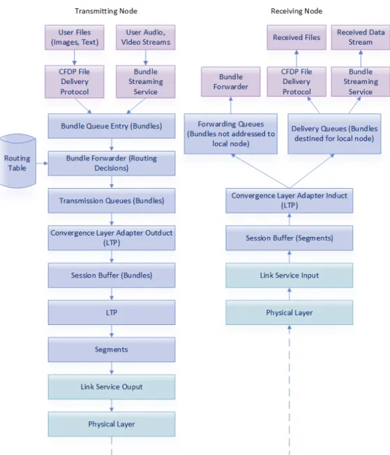
Figure 2.2shows a top level flow chart of one DTN node transmitting data to a receiving node [7]. User applications will generate data such as image or text files which can be sent to a file delivery service such as CFDP (CCSDS File Delivery Protocol) that will segment the files and interact with the bundle proto-col layer. User audio and video data may be sent over a streaming service which will also interact with the bundle layer. Once the data has been formatted into

Figure 2.2. DTN Top Level Flow Chart

bundles via bundle layer library calls (bundle protocol send and receive func-tions), they enter the bundle forwarding queue. The bundle forwarder will ex-amine the bundle header destination, custody transfer requests and time-to-live to determine a suitable path to send the data to its destination. The bundle for-warder/router will consult a routing table with information regarding which of its outgoing queues corresponds to a suitable neighboring node.

Depending on the transport layer that corresponds to the selected outgoing queue, a convergence layer adapter must be selected to encapsulate the bundle into the appropriate protocol data unit. In the case of LTP, a session buffer will be used to store the LTP segments while waiting for acknowledgments from the des-tination node regarding the reception of reliably sent data. Similarly, when data arrives at the receiver, segments enter the LTP session buffer and the appropri-ate convergence layer adapter interacts with the bundle layer. The new bundles are either sent to a forwarding queue if they are destined for another node and sent to a delivery queue if they are addressed to the local node. They will then be reassembled into application data units and received by the appropriate appli-cation at the final destination node.

2.2.2 Bundle Protocol

The format of each bundle consists of at least two blocks, a primary block and a payload block. The first block in a sequence is the primary block which con-tains information about the bundle source, destination, creation time and other processing information. The payload block contains the actual data that is be-ing sent in the bundle. Figures2.3and2.4show examples of the bundle primary and payload blocks. Bundle protocol makes use of Self-Delimiting Numeric Val-ues (SDNVs) for much of its processing information. SDNVs consist of a variable number octets. The last octet has its most significant bit set to zero. The most significant bit of all other octets is set to one. The value encoded in the SDNV is the unsigned binary number obtained by concatenating the seven least signifi-cant bits of each octet [6]. Each field other than the version can be of variable length since they are using the SDNV format.

Figure 2.3. Bundle Protocol Primary Block[6]

Figure 2.4. Bundle Protocol Payload Block[6]

The steps for bundle transmission outlined in the bundle protocol specifica-tion [6] are shown in Figure2.5. A brief summary of the procedure is as follows:

• The forwarder examines the bundle header to see if custody transfer is requested. This means that the local bundle agent must agree to accept-ing custody of the bundle

• Transmission of the bundle begins by creating an outbound bundle with retention constraint “dispatch pending” and the current custodian end-point is set to none.

Figure 2.5. Bundle Protocol Transmission Procedure[6]

• If the bundle is destined for an endpoint to which the node is a mem-ber, the bundle is delivered locally. Otherwise, the bundle forwarding procedure is followed.

• To begin bundle forwarding, the “forward pending” retention constraint is added and the “dispatch pending” constraint is removed. A “retention

constraint” is term used in the protocol for essentially flags added to the bundle’s state designating a reason for which the bundle must continue to be stored and must not be deleted until all retention constraints have been removed.

• It must be determine if forwarding contraindications exist. If the bundle forwarding agent cannot find any endpoint to send the bundle to which moves the bundle towards its destination, forwarding is not possible. In addition, if an endpoint is found to forward the bundle to, an appropri-ate convergence layer adapter must exist that will allow the bundle to be sent to the selected endpoint. If either of these conditions exist, the forwarding contraindicated procedure is followed.

• If forwarding was contraindicated, the bundle protocol agent must de-termine if forwarding has failed, depending on the reason that forward-ing was contraindicated. If it has been determined that forwardforward-ing is not possible, the forwarding failed procedure is followed. Otherwise, the bundle agent will attempt to forward the bundle again at a later time. • If forwarding has failed and custody transfer was requested, a “failed”

custody signal is sent to the bundle’s current custodian, with a reason code corresponding to the forwarding failure reason. If local node is a member of the bundle’s destination endpoint, the “forward pending” re-tention constraint must be removed. The bundle is deleted.

• If custody transfer was requested, the custody transfer procedure is fol-lowed.

• The bundle is sent to each convergence layer adapter for each endpoint selected.

• When each convergence layer adapter has completed, a bundle forward-ing report is sent to the report-to endpoint id requested in the bundle header and the “forward pending” retention constraint is removed.

Figure2.6shows the steps for the bundle reception procedure as outlined in the bundle protocol specification [6]. The steps are summarized as follows:

• The “dispatch pending” retention constraint is added to the bundle. • If “request reporting of bundle reception” is specified, a bundle

recep-tion status report is sent to the bundle’s report-to endpoint id.

• If there are any blocks that are intelligible and cannot be processed, a “block unintelligible” status report is sent if required. The bundle is deleted if the block processing flags indicate to do so.

• If bundle custody transfer was requested, and if it is found that this bun-dle has the same source, timestamp, fragment offset and payload length as an existing bundle, this bundle is redundant. In this case custody transfer redundancy must be handled.

• If the bundle’s destination is the local node, the bundle delivery proce-dure is followed. Otherwise the bundle forwarding proceproce-dure is followed as discussed in the bundle transmission procedure.

• When the bundle has reached its destination endpoint if the bundle is a fragment, the application data unit reassembly procedure is followed. If this results in the completion of an application data unit, the bundle can be delivered. Otherwise, the “reassembly pending” retention constraint is added to the bundle and it must wait for the remaining fragments.

• If the registration corresponding to the destination endpoint id is in the active state, the bundle is delivered. If the registration is in the passive state, then delivery failure results.

• If “request reporting of bundle delivery” was indicated, then a bundle delivery report is generated and sent to the bundles report-to endpoint. If custody transfer was indicated, then a “Succeeded” custody signal is sent to the bundle’s current custodian.

Figure 2.6. Bundle Protocol Reception Procedure[6]

2.2.3 DTN IP Neighbor Discovery

In addition to Bundle Protocol, the DTN protocols also define an opportunis-tic discovery mechanism, IP Neighbor Discovery (IPND)[8]. IPND allows nodes

to announce themselves to previously unknown nodes and exchange connec-tivity information. In this way, it is not necessary to know node addressing and schedules in advance. If two nodes come in contact with one another, they will exchange information using discovery beacons in the form of UDP datagrams.

DTN IP Neighbor Discovery (IPND) is an Internet Draft protocol outlining the mechanism for previously unknown DTN nodes to exchange connectivity infor-mation to allow them to begin to communicate with one another [8]. It utilizes discovery beacons to allow nodes to advertise their existence to one another. The beacons are small UDP datagrams, so that any node using an IP-based conver-gence layer may participate in the discovery process. This is done as part of the Bundle Protocol overlay concept, so that heterogeneous networks may still ex-change data using the commonality of the bundle layer and IP underlay.

IPND beacons are sent periodically to neighboring nodes. They may be either unicast or multicast messages. There is no specification for the time interval be-tween periods, as this is quite application specific and may vary greatly depend-ing on the type of nodes participatdepend-ing in the neighborhood discovery. A beacon period field indicating the frequency at which beacons will be sent is considered optional within the specification. Data sent between discovered nodes may sub-stitute as a beacon, and the reception of data from a discovered node suppresses the output of discovery beacons between the two neighbors [8]. Figure2.7shows the beacon format. The discovery beacon consists of the following fields:

• Version: An 8-bit field representing the IPND version

• Flags: 8 bits which serve as processing flags. The flags indicate if various optional fields are present. A given bit is set if the related field is present

within the beacon. The flags consist of the following, (listed in order of least-signficant-bit to most significant):

– Bit 0: Source Endpoint ID (EID) present

– Bit 1: Service block present

– Bit 2: Neighborhood Bloom Filter present

– Bit 3: Beacon Period present

• Beacon Sequence Number: 16-bit field that is incremented each time a beacon is transmitted to a given IP address.

• EID Length: The byte length of the canonical EID contained in the bea-con.

• Canonical EID: The canonical EID of the node advertised by the beacon. • Service Block: An optional listing containing all or some of the follow-ing information: convergence layers available at the advertised node, a Neighborhood Bloom Filter, routing information and other implemen-tation specific fields.

• Beacon Period: Optional field containing the period at which the adver-tised node will send discovery beacons.

Due to the nature of DTNs and MANETs (Mobile Ad-Hoc Networks), it is not assumed the links are bidirectional. This is because there very often is a dif-ference in antennae characteristics, transmit power and other factors between wireless nodes. For this reason, it is not assumed that just from receiving a bea-con that data may be sent to the neighboring node. IPND uses a Neighborhood Bloom Filter (NBF) to determine the set of neighboring nodes relative to the transmitting node. If the receiving node is contained in the NBF, then it is as-sumed safe to transmit data to that node as the link is considered bi-directional [8].

Determination of link connectivity is left to implementation specific details and not outlined within the IPND specification. Upon receiving a beacon, a node may determine that the neighbor is available to receive data. Continued receipt of beacons within the beacon period specified or data is used to determine the link state. The actual process of establishing a connection between nodes is de-pendent on the lower level protocols used. The convergence layer information listed in the beacon service block will provide the information required to make the connection, such as addresses and port numbers on the listening node.

It has been noted that there are several security concerns regarding IPND, as well as DTNs and neighborhood discovery protocols in general [9], [10], [11]. Since nodes participating in discovery advertise their connectivity information, it is apparent that applications with specific security concerns should not use IPND without implementing a security strategy.

2.3 Machine Learning

Machine learning is a somewhat broad term that can encompass techniques from artificial intelligence, statistics, control theory, and data mining among oth-ers. Machine learning algorithms are often categorized as supervised or unsu-pervised. In supervised learning, a large set of data is used to train the learner. The learner develops rules from the dataset in order to classify new instances of the data based on the training set. Data in the training set is labeled and the learner makes predictions which may be correct or incorrect. In unsupervised learning, the goal is to draw inferences about the input data and learn more about associations within the data set by using techniques based on mathemat-ics and statistmathemat-ics. Unsupervised learning doesn’t develop a set of rules or deci-sion criteria, instead it is used to learn about the characteristics of a dataset. Yet another subset of machine learning is reinforcement learning. In this case, the learner makes decisions initially in a trial-and-error method. Decisions which result in a positive outcome earn the learner a reward. In this way, the learner determines what are good and bad decisions in a given instance. Each of these methods has its own particular strengths and weakness and can be applied to a network routing problem in different ways.

2.3.1 Reinforcement Learning

Reinforcement learning is a subset of machine learning algorithms in which the learner discovers how to best map situations to a desired outcome by max-imizing a numerical reward. The learner is not told what to do, it must learn through a trial and error process to act in a way that maximizes its reward. The

reward may not be immediate, several actions may be completed before the fi-nal reward is received and previous actions may influence future rewards. Rein-forcement learning differs from supervised learning in that there are no exam-ples provided by an external supervisor. In reinforcement learning, the learner must interact with its environment and learn from its own experience [12].

Figure2.8shows an example scenario of a reinforcement learning problem. A robot must learn to navigate through a maze environment. The robot has a current state it determines from the environment and will take a specific action. It will receive a reward based on the action and the next state. If the robot makes a movement that leads it to an open path in the next state, it increases a numerical reward (+10 for example). If the movement leads to being blocked by a wall, it will not receive a reward.

Reinforcement learning systems typically consists of four elements: a policy, a reward function, a value function, and in some cases, a model of the environ-ment [13]. A policy describes the way in which the learner behaves in a given situation. The policy maps the perceived state of the environment to the action the learner will take in that situation. The reward function is based on the goal of the learning problem. Each state is given a reward value that informs the learner about the desirability of that state. The value function defines the total amount of reward the learner can expect to accumulate over time, starting from that state. The reward function specifies the immediate reward, whereas the value function looks ahead to the future rewards the learner will earn based on its previous state. The final element, the model of the environment, can be used by the learner to help to predict the expected rewards as possible next states based on the current state. The learner uses the model to plan its next action [13].

Q-Learning is a reinforcement learning strategy that is classified as temporal-difference learning (TD). Temporal-temporal-difference learning methods can learn di-rectly from experience without a model of the system by which to make predic-tions. This type of learner bootstraps, meaning it updates its estimates based on other learned estimates without waiting for the final outcome or receiving its final reward [13].

Q-Learning itself is a fairly simple approach. The Q-Learning algorithm is defined by st , a non-terminal state visited at timet, the learned action-value

function Q, and an action a. Q-Learning chooses the next action that will be taken by selecting the one which will maximize its current reward and the future rewards it expects to learn. The current value in Q-table is updated after the action is taken and the algorithm proceeds recursively to make the next decision

and update to the Q-Table. Pseudo code for the basic Q–Learning algorithm is given in Algorithm 1. In this listing,ris the reward at timet, andγis the discount rate parameter between 0 and 1[12].

Algorithm 1. Q-Learning Pseudocode [12] I n i t i a l i z e Q( s , a ) a r b i t r a r i l y

ForEach( episode ) : I n i t i a l i z e s

ForEach( s t e p o f each episode ) :

Choose a from s using p o l i c y derived from Q Take action a , r e c e i v e reward r

Observe new s t a t e st+1

Q(s,a)←r+γmaxat+1Q(st+1,at+1) s←st+1

Until s i s terminal

The Q-learning algorithm utilizes a table comprised of entries representing the reward associated with every possible state-action pair. Initially, all entries are initialized to zero or a random value. The learning agent must estimate the reward associated with each state-action pair. From the Q-table the agent will se-lect the action that maximizes its reward at the current time. After it has sese-lected an action, the learner will update its Q-table with the reward it received. This is intended to improve the estimates of the Q-table and allow the learner to con-stantly tune its policy to receive better rewards. After many iterations, the agent will converge to an optimal policy, though in some cases this may take several thousands of iterations [14].

2.3.2 Classification

Classification is a method of categorizing objects as having a set of attributes and an overall label which describe it. Labels typically consist of a finite set of discrete values. Attributes are a vector of several values which also are typically

discrete, but may also be continuous values that are divided into discrete bins. Previous pairs of attributes and labels can be used to make predictions about new instances of objects. In the simplest classification methods, the frequency of occurrence of a certain set of attributes appears with a given label can be used to determine the most likely label for a new instance with similar attributes.

The performance of a classification algorithm can be measured in several ways. Typically, a data set that is being used to develop a classification model will be divided into several training and test sets. The training set(s) will be used to allow the algorithm to learn which labels coincide with a given set of attribute values. This will allow the algorithm to construct a model of the data set. Once the algorithm has been trained, it will be executed on the test data set, which the trained model currently has no knowledge of. The algorithm will only be given access to the attribute values and must predict what label to assign to a new data point. Once this is completed the number of correct classifications can be deter-mined by comparing the algorithm output to the set of known labels that were withheld during the testing phase. In addition to simply counting correct classifi-cations versus incorrect classificlassifi-cations, the performance can be evaluated using precision and recall. Precision and recall are calculated by counting the total true positivestp, true negativestn, false negatives fnand false positives fp for

exam-ples classified as labell. The F1 score is as a weighted average of the precision and recall. Each of these metrics are discussed in more detail in Chapter 7.

There are several well known and rather simple classification techniques used in this research. Decision trees, K-Nearest Neighbors, Naive Bayes were used to classify neighboring nodes in terms of route suitability. This section will briefly discuss the basic concepts of each.

Decision Trees

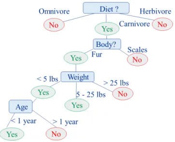
Decision trees construct a graph like tree structure based on a series of yes or no decision criteria as learned by associating frequency of occurrences of a specific label value with a specific attribute value. The ID3 decision tree algo-rithm uses information gain, a function based on the entropy of training data set to determine which attributes should be used as the root decision of the tree, following down through the lower branches of the tree [12]. Information gain is used to determine the relevance of each variable to predicting the category label, it is the amount of information gained about the label from observing a specific attribute. The attribute which has the greatest information gain is selected as the root node, and is the evaluated recursively to generate the rest of the tree struc-ture. The entropy of a data setSis defined as:

Ent r op y(S)≡ −p_⊕log₂p_⊕−p_ªlog₂p_ª (2.1)

wherep_⊕andp_ªare the proportion of positive and negative examples inS. From the entropy, information gain can be obtained in Eq. 2.2:

G ai n(S,A)≡Ent r op y(S)− X

v∈V al ues(A) |Sv|

|S| Ent r op y(Sv) (2.2) Figure 2.9shows an example of the decision tree structure that could be used to classify types of animals. Each node in the tree examines the attributes of an animal and the value of the attributes contribute to the determination of a binary decision on whether or not it is a specific type of animal (in this case, a small carnivorous animal like a cat).

Figure 2.9. Decision Tree Illustration

Naïve Bayes

The concept of Bayesian machine learning is based on the conditional prob-ability that a certain outcome has some likelihood given that it possesses a par-ticular set of attributes. This learning method is used to classify a new instance or occurrence within a set of possible values based on previous training data. The learner will determine the probability that a certain set of attributes most likely correspond to a specific classification within the training data. When a new occurrence is presented to the learner, the training probabilities are used to determine the valuevof the new instance from a finite set of valuesV based on its attribute vector<a1,a2, ...,an >[12]. There are many benefits to the Naïve

Bayes classifier in that it is a very simple method and performance is generally not affected by missing attributes. It has been used for many classification prob-lems and is particularly well known for categorizing text based on words within the text. In this example, the learner will predict what the text is about based on the frequency that certain words (the attributes) appear within the text [12].

Bayesian learning is based on calculating the most probable outcome, often called the maximum a posteriori or MAP hypothesis. The Naïve Bayes classifier attempts to find the most probable value for a current instanceVM AP given its

known attributes<a1,a2, ...,an>[12].

VM AP =max vj∈V

P(vj|a1,a2, ...,an) (2.3)

Bayes rule can be used to write Eq. 2.3 as:

VM AP =max vj∈V

P(a1,a2, ...,an|vj)P(vj) P(a1,a2, ...,an)

(2.4) The termP(a1,a2, ...,an) is dropped since it is a constant independent ofvj.

This simplifies to:

VM AP=P(a1,a2, ...,an|vj)P(vj) (2.5)

Equation 2.5 calculates the MAP hypothesis as the probabilities of observing the value vj in conjunction with the attributes <a1,a2, ...,an >. This is easily

found by taking the product of the conditional probabilities of observingvjgiven

each individual attribute. The Naïve Bayes classifier becomes [12]:

VN B=max vj∈V P(vj) Y i P(ai|vj) (2.6) K-Nearest Neighbors

K-Nearest Neighbors is a classification method which classifies objects based on a distance measure relative to other instances in the data set. The attribute vector<a1,a2, ...,an)>can be thought of as x, y coordinates on a plot and each

point will have its associated label. The distance will be calculated from a new point <b1,b2, ...,bn>to all the other neighboring points .The actual attribute

vector can consist of more than two dimensions and this will not affect the dis-tance formula, simply more attributes are added. Euclidean disdis-tanced(a,b)≡ s

n

P

i=1

(ai−bi)2 can be used as well as other distance metrics. The number of

neighbors selected for the distance calculation is the number K, the K nearest neighbors to the point are chosen for the classification. The new point will be classified as the label that most frequently occurs among the K nearest neigh-bors. Figure2.10shows a graphical representation of classifying a new data point indicated by either a white or black x, representing a binary label such as true/-false or positive/negative based on its 5 closest neighboring points.

Figure 2.10. K-Nearest Neighbors Illustration

2.3.3 Multi-label Learning and Metrics

The classification methods described in the previous section discusses meth-ods which produce a single label , either binary or selected from a finite set of possible labels, for a single instance of an attribute vector. Multi-label classifica-tion allows for there to be multiple categories of labels assigned to one instance

of an object. An example of this could be in the classification of books. A multi-label classification of a book could be non-fiction, paperback, and biography. There are several approaches to multi-label classification that were used in this dissertation.

The simplest form of multi-label classification is the Binary Relevance (BR) method. In this case the multi-label classification is decomposed into several bi-nary classifications, one for each label category. This can be considered a prob-lem transformation approach. A single classification probprob-lem with multiple out-puts is transformed into multiple classification problems. This method has been critiqued for the fact that all labels are classified independently, without taking into account interdependence between outputs.

A large amount of work in multi-label classification has been focused on de-termining the relationships between labels to improve classification accuracy. Classifier Chains [15] (CC) also transform the multi-label problem into a set of individual binary classifications, however the attribute space for each model is extended with the binary label relevances of all previous classifiers, forming a chain. This takes associations between previously classified labels into account when performing classification of the next label. For this reason, selection of the order in which labels are classified may influence the outcome of how the classifier performs. A poor choice of order can negatively impact performance. In addition, one drawback of the CC approach is that errors can be propagated through the chain, for example by the early choice of a poor order further im-pacting the performance down the rest of the chain. The Ensemble of Classifier Chains (ECC) attempts to correct this issue by using multiple chains of randomly

ordered classifiers, so that the impact of order selection will be decreased overall [15].

To validate the multi-label classification performance, there are four well known multi-label prediction metrics used. Hamming loss calculates the fraction of la-bels that are incorrectly classified. This is in contrast to zero-one loss which con-siders the entire prediction incorrect if any label in the prediction is incorrect. Hamming loss is a more lenient metric which scores based on individual labels. In both Hamming loss and zero-one loss, values tending toward zero indicate good performance whereas values tending toward one indicate a higher percent-age of misclassification. The Jaccard similarity score is the size of the intersection of two label sets ( the predictions and true labels) divided by the size of the union of the two label sets. The F1 score is as a weighted average of the precision and recall. Micro-average F1 score calculates the score globally by counting the total true positives, false negatives and false positives. These metrics are discussed in detail in Chapter 7.

2.3.4 Clustering

Clustering is an unsupervised learning method which can be used to deter-mine how similar two or more attribute vectors are two each other. The method used in this dissertation was the K-Means Clustering algorithm [16], which pro-duces disjoint clusters. The attributes within the data set can be thought of as points on an x, y plot. Initially,K cluster centers are randomly selected among the possible x, y coordinates. Each point ion the data set is assigned to the cluster whose center is closest. Next, theK cluster centers are recalculated as the mean of the coordinates of each cluster. All of the points are reassigned based on the

new cluster centers, and the process repeats until the cluster centers no longer change. An understanding of the data set can be developed from information about what points have been clustered together.

Equation (2.7) shows how the clusters are calculated [17]. The goal is to min-imize J, the sum of squares of the distances of each point to the centroid of its assigned clusterµk. HereK is the number of clusters,N is the number of data

points and xn is each data point to be clustered. The variablernk is an binary

indicator of whether the point xn should be assigned to cluster k as shown in

Equation (2.8). J= N X n=1 K X k=1 rnk ° °x_n−µ_k ° ° 2 (2.7) rnk=          1 k=ar g mi nj ° °x_n−µ_j ° ° 2 0 ot her wi se. (2.8)

An iterative procedure is used to find values of the cluster centersµkandrnk

3

Related Work

This section covers several routing algorithms that were closely related to and/or used in this dissertation. Algorithms such as flooding, epidemic and PRoPHET are well known in the DTN community and often used as points of ref-erence or the basis for new routing approaches. In addition, several lesser known works that are closely related to the topic of machine learning in regard to DTNs are also covered.

3.1 DTN Routing Algorithms

Balasubramanian et al. classify most DTN routing protocols as either based on packet forwarding or packet replication [18]. Replication based routing, or epidemic routing protocols, create multiple copies of a packet to send to neigh-boring nodes with the intent that the packet will traverse multiple paths and have a greater likelihood to reach its final destination. Forwarding based routing pro-tocols create a single instance of a packet and employ various methods to deter-mine a suitable path, often requiring global knowledge of the network.

In the case of a space network, it can be seen that both of these approaches have their own benefits and drawbacks. As noted in [18], naïve flooding can con-sume excessive resources on any node by generating multiple copies of unneces-sary bundles. In the case of satellite networks, on-board avionics are often quite processor and memory limited, making this unnecessary processing particularly troublesome. Benefits of replication include redundancy to prevent lost pack-ets, and potentially simplified algorithms which require limited knowledge of the global network. The need for feedback regarding the network state in particular can be impractical for deep space communication, where information will likely be stale by the time it reaches its destination. In contrast, while forwarding-based protocols require fewer resources, they often have lower message delivery rates [19]. Furthermore, the use of an oracle with future knowledge of the network, or a knowledge base of the existing network may be difficult to implement in many real-life scenarios [18].

Table3.1shows a comparison of the routing algorithms studied in this work. The column "Replication" indicates if the algorithm uses message replication or it forwards a single copy. The column "Topology" lists the intended type of network topology, meaning a fairly randomly changing topology, a more sta-ble graph-like topology and changing topologies particularly focused on VANETs (Vehicular Ad hoc Networks). The final column "Methodology" is a brief sum-mary of the main routing mechanism. The five algorithms listed first (epidemic, DTLSR, PRoPHET, RAPID and CGR) are very well known DTN routing algorithms. The next two listed (Bayesian and Epidemic+C and Saw+C) are lesser known but

included due to the similarity and relevance to this work. The final two algo-rithms (Classification and Clustering) are the algoalgo-rithms developed in this dis-sertation.

Algorithm Replication Topology Methodology

Epidemic Replication Frequently Changing Replicate unknown bundles DTLSR Forwarding Relatively Stable Link state announcements PRoPHET Replication Changing Probabilistic history of encounters RAPID Replication VANET Maximize utility metric

CGR Forwarding Relatively Stable Forward based on contact schedule Bayesian [20] Replication VANET Bayesian classification

Epidemic+C/SaW+C [21] Replication VANET Decision tree

Classification Replication Frequently Changing Ensemble of classifiers

Clustering Replication Frequently Changing Cluster analysis by node location Table 3.1. Summary of DTN Routing Algorithms

3.1.1 Flooding/Epidemic Routing

Flooding or epidemic routing is the simplest type of routing, aside from stat-ically configured routes. Epidemic routing schemes assume minimal knowledge of the network topology. Messages are replicated each time the transmitting node comes in contact with a new neighboring node [22]. This approach has a high delivery probability and low delay, however it consumes a great deal of resources in terms of message storage and utilizing transmission opportunities for messages that already exist in the network. Nodes will need to determine when copies should be deleted and how to deal with receiving duplicate mes-sages. Furthermore, this approach will not scale well with a large amount of data or a large number of nodes. Solving these issues has given rise to an entire class of epidemic-based routing algorithms. Spray-and-Wait [23] is one such approach in which the transmitting node begins with an initial "spray" phase where copies of each message are sent to each available relay node. The transmitting node

then waits to see if one of the relay nodes was the message destination, if not the relay nodes will wait to see if they can forward the message on to its destination.

3.1.2 DTLSR

Delay Tolerant Link State Routing (DTLSR) is based on conventional link state routing [24]. Nodes attempt to learn the network topology by sending flooding messages containing connectivity information for the current state of the net-work. The network topology is stored by each node in the form of a network graph. Routes are computed using Dijkstra’s shortest path algorithm. Link State Announcement messages may contain the source node’s endpoint identifier, se-quence number and link state information such as the next hop destination and queue status. DTLSR differs from standard link-state routing (LSR) in that cur-rently unavailable nodes are still considered in the best path computation. For nodes that are available, hop count can be used as a simple metric to determine the best path. This does not allow the algorithm to take advantage of better paths that may not currently be available but will be in the future when the message arrives at a remote node. To account for this, DTLSR attempts to minimize the estimated expected delay. For nodes that are available, the delay is estimated based on the total size of all messages in the queueql en (bits), number of

mes-sages in the link queueqnum, the per-message latency (s) and bandwidth (bps).

The estimated delay is given by Eq. 3.1 [25]:

d el a yav ai l abl e=qnum×l at enc y+

q_{l en}

band w i d t h (3.1)

The estimated delay associated with unavailable nodes is inferred from the duration of the current outage. This is based on the assumption that if a node

has been unavailable for a long amount of time, it is likely to continue to be un-available. The duration is limited to 24 hours [24].

3.1.3 PRoPHET

The PRoPHET (Probabilistic Routing Protocol using History of Encounters and Transitivity) routing protocol attempts to reduce the number of replicated bundles in the network by calculating the probability of successful message de-livery to a given destination. PRoPHET is based on the human mobility model and the observation that a large number of contact opportunities between two nodes follow a non-random pattern [26]. Messages are replicated and sent to neighboring nodes that have a high probability of delivering it to its destination. PRoPHET determines this likelihood based on a delivery predictability metric. Each node maintains a vector of delivery predictabilities for all nodes encoun-tered and exchanges this information with other nodes during an initial contact phase. The delivery predictability is calculated whenever two nodes are in con-tact. Nodes which are frequently in contact have a higher delivery predictability and as such the algorithm will choose that pair of nodes as the preferred path. The delivery predictability P(A,B) for node A to destinationB is calculated as follows [27]:

P(A,B)=P(A,B)ol d+(1−P(A,B)ol d)×Penc≤1 (3.2)

The probability of direct encounter Penc is a configurable parameter meant to

increase the delivery probability of nodes that are frequently encountered. De-livery predictabilities for other nodes encountered byB are updated for node A

using the transitive property. The transitive property is based on the concept that if nodeA frequently encountersB and nodeB frequently encounters node