Performance benchmarking, analysis, and optimization of deep learning inference

(1)

(2)

PERFORMANCE BENCHMARKING, ANALYSIS AND OPTIMIZATION OF DEEP LEARNING INFERENCE

BY CHENG LI

DISSERTATION

Submitted in partial fulfillment of the requirements for the degree of Doctor of Philosophy in Computer Science

in the Graduate College of the

University of Illinois at Urbana-Champaign, 2020

Urbana, Illinois

Doctoral Committee:

Professor Wen-mei Hwu, Chair

Assistant Professor Christopher W. Fletcher Professor David A. Padua

(3)

ABSTRACT

The world sees a proliferation of deep learning (DL) models and their wide adoption in dif-ferent application domains. This has made the performance benchmarking, understanding, and optimization of DL inference an increasingly pressing task for both hardware designers and system providers, as they would like to offer the best possible computing system to serve DL models with the desired latency, throughput, and energy requirements while maximizing resource utilization. However, DL faces the following challenges in performance engineering. Benchmarking— While there have been significant efforts to develop benchmark suites that evaluate widely used DL models, developing, maintaining, and running benchmarks takes a non-trivial amount of effort, and DL benchmarking has been hampered in part due to the lack of representative and up-to-date benchmarking suites.

Performance Understanding — Understanding the performance of DL workloads is challenging as their characteristics depend on the interplay between the models, frameworks, system libraries, and the hardware (or the HW/SW stack). Existing profiling tools are disjoint, however, and only focus on profiling within a particular level of the stack. This largely limits the types of analysis that can be performed on model execution.

Optimization Advising— The current DL optimization process is manual and ad-hoc that requires a lot of effort and expertise. Existing tools lack the highly desired abilities to characterize ideal performance, identify sources of inefficiency, and quantify the benefits of potential optimizations. Such deficiencies have led to slow DL characterization/optimization cycles that cannot keep up with the fast pace at which new DL innovations are introduced. Evaluation and Comparison— The current DL landscape is fast-paced and is rife with non-uniform models, hardware/software (HW/SW) stacks, but lacks a DL benchmarking platform to facilitate evaluation and comparison of DL innovations, be it models, frameworks, libraries, or hardware. Due to the lack of a benchmarking platform, the current practice of evaluating the benefits of proposed DL innovations is both arduous and error-prone — stifling the adoption of the innovations.

This thesis addresses the above challenges in DL performance engineering. First we in-troduce DLBricks, a composable benchmark generation design that reduces the effort of developing, maintaining, and running DL benchmarks. DLBricks decomposes DL models into a set of unique runnable networks and constructs the original model’s performance us-ing the performance of the generated benchmarks. Then, we present XSP, an across-stack profiling design that correlates profiles from different sources to obtain a holistic and

(4)

hier-archical view of DL model execution. XSP innovatively leverages distributed tracing and accurately capture the profiles at each level of the HW/SW stack in spite of profiling over-head. Next, we propose Benanza, a systematic DL benchmarking and analysis design that guides researchers to potential optimization opportunities and assesses hypothetical execu-tion scenarios on GPUs. Finally, we design MLModelScope, a consistent, reproducible, and scalable DL benchmarking platform to facilitate evaluation and comparison of DL innova-tions. This thesis also briefly discusses TrIMS, TOPS, and CommScope which are developed based on the needs observed from the performance benchmarking and optimization work to solve relevant problems in the DL domain.

(5)

(6)

ACKNOWLEDGMENTS

Foremost, I would like to thank my advisor Professor Wen-mei Hwu for his support of my Ph.D. study. Five years ago, Wen-mei kindly admitted me to University of Illinois at Urbana-Champaign (UIUC). I am honored to be a member of the IMPACT (Illinois Microarchitecture Project using Algorithms and Compiler Technology) Research Group ever since. Wen-mei provided me with valuable guidance on my research. He also encouraged and sponsored me to attend many conferences and events to present my work and get inspired. Without Wen-mei, I could not have made it here and become a researcher.

Besides my advisor, I would also like to thank the rest of my doctoral committee: Assistant Professor Christopher W. Fletcher, Professor David A. Padua, and Dr. Wei Tan, for their insightful comments and suggestions on my thesis work.

Next I would like to thank Abdul Dakkak, my colleague and collaborator, for teaching me a lot of research/engineering skills that I will benefit from for the rest of my life. As a senior member of the research group, Abdul did a great job mentoring me. I am also deeply grateful to other group members for their support and companionship in this journey.

My sincere thanks also go to my collaborator Jinjun Xiong at IBM Research. Jinjun is a very good researcher and gives useful feedback on many of my research projects. He is always willing to help. There were many times when I worked on paper submissions with tight dealings and Jinjin helped as much as he could until the last minute.

Finally, I would like to acknowledge with gratitude, the love and support of my family — my parents, Ruihai and Huazhi; my brother and his wife, Bo and Xiaoxu. They are always there for me no matter what happens. Without their encouragement, I would not have overcome the challenges I encountered during my study. This thesis would not have been possible without them. I am extremely lucky to have them in my life.

(7)

CHAPTER 6 MLMODELSCOPE: THE DESIGN AND IMPLEMENTATION OF A SCALABLE DL BENCHMARKING PLATFORM . . . 74

6.1 Design Objectives . . . 76

6.2 MLModelScope Design and Implementation . . . 78

CHAPTER 7 OTHER RELEVANT WORKS . . . 96

7.1 TrIMS: Transparent and Isolated Model Sharing for DL Inference . . . 96

7.2 TOPS: Accelerating Reduction and Scan Using Tensor Core Units . . . 99

(8)

CHAPTER 8 CONCLUSION . . . 103 REFERENCES . . . 104

(9)

CHAPTER 1: INTRODUCTION

The past few years have seen a spur of deep learning (DL) innovations. These innovations span from DL models to software stack optimizations (e.g., frameworks such as MXNet or PyTorch, libraries such as cuDNN or MKL-DNN) and hardware stack improvements (e.g. CPU, GPU, FPGA). Among all the innovations, however, DL models are the most rapidly evolving and prolific. This is true in both academia [1] and industry [2], where models are tweaked and introduced on a weekly, daily, or even hourly basis. There have been numerous impressive advances in applying DL in many application domains such as image classification, object detection, machine translation, etc.

This has resulted in a surge of interest in deploying these DL models within various computing platforms/devices including commodity servers, accelerators, reconfigurable hard-ware, mobile and edge devices. Therefore, there is an increasing need for hardware providers, computer architects, and system/chip designers to benchmark, understand and optimize DL model inference performance (throughput, latency, system resource utilization, etc.) across different computing systems. However, DL inference performance engineering faces the fol-lowing challenges, which stifle the adoption of DL innovations.

Developing, maintaining, and running DL benchmarks — For each DL task of interest, benchmark suite authors select a small subset (or one) out of tens or even hundreds of candidate models. Deciding on a representative set of models is an arduous effort as it takes a long debating process to determine what models to add and what to exclude. For example, it took over a year of weekly discussion to determine and publish MLPerf v0.5 inference models, and the number of models was reduced from the 10 models originally considered to 5. Given that DL models are proposed or updated on a daily basis [1, 2], it is very challenging for benchmark suites to be agile and remain representative of real-world DL model usage. Moreover, only publicly available models are considered for inclusion in benchmark suites. Proprietary models are trade secrets or restricted by copyright and cannot be shared externally for benchmarking. Thus, proprietary models are not included or represented within benchmark suites. Due to these issues, DL benchmarking has been hampered in part due to the lack of representative and up-to-date benchmarking suites.

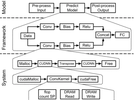
Understanding DL performance across the hardware/software stack — DL model inference is complex and its performance is impacted by the interplay between differ-ent levels within the hardware/software (HW/SW) stack — frameworks, system libraries, and hardware. An example is shown in Figure 1.1. Due to the complexity of model execu-tion, to be able to identify bottlenecks and locate their sources, one needs a holistic view

(10)

Pre-proess Input Post-process Output Predict Model Conv Conv Bias Concat Bias Data FC Relu Relu

Malloc CUDNN Transpose CUDNN Free

flop count SP DRAM Read DRAM Write cudaMalloc ConvKernel cudaFree

Mo de l F ra me w ork Syst em

Figure 1.1: DL model performance is impacted by the interplay between different levels within the HW/SW stack - frameworks, system libraries, and hardware.

of the model execution. However, existing profiling tools or methods only provide partial views of model execution.

Interpreting DL benchmarking results into possible optimizations — Both in-dustry and academia have invested heavily in developing benchmarks to characterize DL models and systems [3–7]. The characterization is followed by optimization to improve the model performance. However, there is currently a gap between the benchmarking re-sults and possible optimizations to perform. Researchers use profilers, such as nvprof [8], Nsight [9], and VTune [10], to profile DL model execution and get low-level GPU and CPU information. With ample knowledge of how models execute and utilize system resources, researchers manually identify bottlenecks and inefficiencies within model execution by ex-amining the profiling results. Researchers then make hypotheses of solutions and try out different ideas to optimize the model execution — which may or may not pan out. This manual and ad-hoc process requires a lot of effort, expertise, and guesswork, and slows down the turnaround time for model optimization and system tuning. Thus, there is a need for a systematic DL benchmarking and subsequent analysis design that can guide researchers to optimization opportunities and assess hypothetical execution scenarios.

Consistent, reproducible, and scalable DL experimentation— The DL landscape is fast-paced and is rife with non-uniform models, HW/SW stacks, but lacks a DL experimen-tation platform to facilitate the evaluation and comparison of DL innovations, be it models, frameworks, libraries, or hardware. To consistently evaluate two DL benchmarks requires one

(11)

to use the same evaluation code and HW/SW environment. However, DL benchmarks are often developed independently as a set of ad-hoc scripts. Thus, a fair comparison requires a non-trivial amount of effort. Furthermore, DL benchmarking often requires evaluating models across different combinations of HW/SW stacks. As HW/SW stacks are increasingly being proposed, there is an urging need for a DL benchmarking platform that consistently evaluates and compares different DL models across HW/SW stacks, while coping with the fast-paced and diverse landscape of DL.

The thesis addresses the above challenges through novel DL benchmarking, analysis, and optimization designs, and is organized as follows:

• Chapter 2 describes DL inference in detail.

• Chapter 3 presents DLBricks, a composable benchmark generation design that decom-poses DL models into a set of unique runnable networks and constructs the original model’s inference performance using the performance of the generated benchmarks. DLBricks reduces the effort to develope, maintain, and run DL benchmarks.

• Chapter 4 presents XSP, an across-stack profiling design that innovatively leverages distributed tracing to construct a holistic and hierarchical view of DL model execution without modification to frameworks. XSP accurately captures the profiles at each level of the stack in spite of the profiling overhead incurred from the profilers. XSP addresses the challenge of understanding DL performance across the HW/SW stack and provides insights that are difficult to discern without it.

• Chapter 5 presents Benanza, a systematic DL benchmarking and analysis design to inform DL inference optimizations on GPUs. Benanza automatically generates micro-benchmarks given a set of models, computes their “lower-bound” latencies using the benchmark data, and informs optimizations of their executions on GPUs. Benanza guides researchers to optimization opportunities and assesses hypothetical execution scenarios on GPUs.

• Chapter 6 presents MLModelScope, a consistent, reproducible, and scalable DL ex-perimentation platform to facilitate evaluation and comparison of DL innovations. MLModelScope offers a unified and holistic way to evaluate, compare and introspect DL inference, and provides an automated analysis and reporting workflow to summa-rize the results.

• Chapter 7 discusses several other works relevant to DL performance which include TrIMS — removing the model loading overhead from the DL inference by exploiting

(12)

sharing of models across the memory hierarchy in the cloud, TOPS — leveraging Tensor Core Units to accelerate non-GEMM primitives that are common in DL operators, and CommScope — understanding memory transfer behavior across different data placement and exchange scenarios.

(13)

CHAPTER 2: DL INFERENCE

A DL model is defined by its graph topology and its weights. The graph topology is defined as a set of nodes where each node is a function operator with the implementation provided by a framework (e.g. TensorFlow, MXNet, PyTorch). A DL inference pipeline includes the pre-processing, prediction, and post-processing steps. Pre-processing is the process of transforming the user input into a form that can be consumed by the model and post-processing is the process of transforming the model’s output to compute metrics. If we take image classification shown in Figure 2.1 as an example, the pre-processing step decodes the input image into a tensor of dimensions [batch,height, width, channel] ([N,H,W,C]), then performs resizing, normalization, etc. The image classification model’s output is a tensor of dimensions [batch∗ numClasses] which is sorted to get the top K predictions (label with probability).

In the model prediction step, the framework acts as a “runtime” and maps the function operators into system library calls. The layers executed by a framework are pipelines of system library calls. The system libraries, in turn, invoke a chain of primitive kernels that impact the underlying hardware counters. As can be observed, this inference pipeline is intricate and has many levels of abstraction — frameworks, system libraries, and hardware, as summarized in Figure 1.1. DL inference performance is impacted by the interplay between these different HW/SW stack levels. When a slowdown is observed, any one of them can be suspect.

(14)

CHAPTER 3: DLBRICKS: COMPOSABLE BENCHMARK GENERATION TO REDUCE DEEP LEARNING BENCHMARKING EFFORT

This chapter presents DLBricks, a composable benchmark generation design that reduces the effort of developing, maintaining, and running DL benchmarks. DLBricks decomposes DL models into a set of unique runnable networks and constructs the original model’s per-formance using the perper-formance of the generated benchmarks. DLBricks can keep up-to-date with the latest proposed models, relieving the pressure of selecting representative DL models.

The recent progress made by Deep Learning (DL) in a wide array of applications, such as autonomous vehicles, face recognition, object detection, machine translation, fraud detec-tion, etc., has led to increased public interest in DL models. Benchmarking these trained DL models before deployment is critical, as DL models must meet target latency and re-source constraints. Hence, there have been significant efforts to develop benchmark suites that evaluate widely used DL models [3, 4, 11, 12]. An example is MLPerf [3], which is formed as a collaboration between industry and academia and aims to provide referfence implementations for DL model training and inference.

However, developing, maintaining, and running benchmarks takes a non-trivial amount of effort. For each DL task of interest, benchmark suite authors select a small representative subset (or one) out of tens or even hundreds of candidate models. Deciding on a representa-tive set of models is an arduous effort as it takes a long debating process to determine what models to add and what to exclude. For example, it took over a year of weekly discussion to determine and publish MLPerf v0.5 inference models, and the number of models was reduced from the 10 models originally considered to 5. Figure 3.1 shows the gap between the number of DL papers [13] and the number of models included in recent benchmarking efforts. Given that DL models are proposed or updated on a daily basis [1, 2], it is very chal-lenging for benchmark suites to be agile and representative of real-world DL model usage. Moreover, only public available models are considered for inclusion in benchmark suites. Proprietary models are trade secrets or restricted by copyright and cannot be shared exter-nally for benchmarking. Thus, proprietary models are not included or represented within benchmark suites.

To address the above issues, we propose DLBricks — a composable benchmark generation design that reduces the effort to develop, maintain, and run DL benchmarks. Given a set of DL models, DLBricks parses them into a set of atomic (i.e. non-overlapping) unique layer sequences based on the user-specified benchmark granularity (G). A layer sequence is a chain of layers. Two layer sequences are considered the same (i.e. not unique) if they are

(15)

��

�

��

�

��

#

��

#

��

Figure 3.1: The number of DL models included in the recent published DL benchmark suites (Fathom [11], DawnBench [6], TBD [12], AI Matrix [4], and MLPerf [3]) compared to the number of DL papers published in the same year (using Scopus Preview [13]) .

identical ignoring their weight values. DLBricks then generates unique runnable networks (i.e. subgraphs of the model with at most G layers that can be executed by a framework) using the layer sequences’ information, and these networks form the representative set of benchmarks for the input models. Users run the generated benchmarks on a system of interest and DLBricks uses the benchmark results to construct a performance estimate on that system.

DLBricks leverages two key observations on DL inference: 1 Layers are the performance building blocks of the model performance. 2Layers (considering their layer type, shape, and parameters, but ignoring the weights) are extensively repeated within and across DL models. DLBricks uses both observations to generate a representative benchmark suite, minimize the time to benchmark, and estimate a model’s performance from layer sequences.

Since benchmarks are generated automatically by DLBricks, benchmark development and maintenance effort are greatly reduced. DLBricks is defined by a set of simple consistent principles and can be used to benchmark and characterize a broad range of models. Moreover, since each generated benchmark represents only the nodes of the input model, the input model’s topology does not appear in the output benchmarks. This, along with the fact that “fake” or dummy models can be inserted into the set of input models, means that the generated benchmarks can represent proprietary models without the concern of revealing proprietary models.

In summary, this work makes the following contributions:

• We perform a comprehensive performance analysis of 50 state-of-the-art DL models on CPUs and observe that layers are the performance building blocks of DL models, thus a model’s performance can be estimated using the performance of its layers (Section 3.1.1).

(16)

• We also perform an in-depth DL architecture analysis of the DL models and make the observation that DL layers with the same type, shape, and parameters are repeated exten-sively within and across models (Section 3.1.2).

• We propose DLBricks, a composable benchmark generation design that decomposes DL models into a set of unique runnable networks and constructs the original model’s perfor-mance using the perforperfor-mance of the generated benchmarks (Section 3.2).

• We evaluate DLBricks using 50 MXNet models spanning 5 DL tasks on 4 representative CPU systems (Section 3.3). We show that DLBricks provides a tight performance estimate for DL models and reduces the benchmarking time across systems. The composed model latency is within 95% of the actual performance while up to 4.4×reduction in benchmarking time is achieved on the Amazon EC2 c5.xlarge system.

This chapter is structured as follows. First, we detail two key observations that enable our design in Section 3.1. We then propose DLBricks in Section 3.2 and describe how it provides a streamlined benchmark generation workflow which lowers the effort to benchmark. Section 3.3 evaluates using 50 models running on 4 systems. In Section 3.4 we describe different benchmarking approaches previously performed. We then describe future work in Section 3.5 before we conclude in Section 3.6.

3.1 MOTIVATION

DLBricks is designed based on two key observations presented in this section. To demon-strate and support these observations, we perform a comprehensive performance and archi-tecture analysis of state-of-the-art DL models. The evaluations in this section use 50 MXNet models of different DL tasks (listed in Table 3.1) and were run with MXNet (v1.5.1 MKL release) on an Amazon c5.2xlarge instance (as listed in Table 3.2). We focus on latency sensitive (batch size = 1) DL inference on CPUs.

3.1.1 Layers as the Performance Building Blocks

A DL model is a directed acyclic graph (DAG) where each vertex within the DAG is a layer (i.e. operator, such as convolution, batchnormalization, pooling, element-wise, softmax) and an edge represents the transfer of data. For a DL model, a layer sequence is defined as a simple path within the DAG containing one or more vertices. A subgraph, on the other hand, is defined as a DAG composed of one or more layers within the model (i.e. subgraph is a superset of layer sequence, and may or may not be a simple path). We are

(17)

Table 3.1: The 50 MXNet models [14] used for evaluation, including Image Classification (IC), Image Processing (IP), Object Detection (OD), Regression (RG) and Semantic Segmentation (SS) tasks.

ID Name Task _LayersNum

1 Ademxapp Model A Trained on ImageNet Competition Data IC 142

2 Age Estimation VGG-16 Trained on IMDB-WIKI and Looking at People Data IC 40

3 Age Estimation VGG-16 Trained on IMDB-WIKI Data IC 40

4 CapsNet Trained on MNIST Data IC 53

5 Gender Prediction VGG-16 Trained on IMDB-WIKI Data IC 40

6 Inception V1 Trained on Extended Salient Object Subitizing Data IC 147

7 Inception V1 Trained on ImageNet Competition Data IC 147

8 Inception V1 Trained on Places365 Data IC 147

9 Inception V3 Trained on ImageNet Competition Data IC 311

10 MobileNet V2 Trained on ImageNet Competition Data IC 153

11 ResNet-101 Trained on ImageNet Competition Data IC 347

12 ResNet-101 Trained on YFCC100m Geotagged Data IC 344

15 Squeeze-and-Excitation Net Trained on ImageNet Competition Data IC 874

16 SqueezeNet V1.1 Trained on ImageNet Competition Data IC 69

17 VGG-16 Trained on ImageNet Competition Data IC 40

18 VGG-19 Trained on ImageNet Competition Data IC 46

19 Wide ResNet-50-2 Trained on ImageNet Competition Data IC 176

20 Wolfram ImageIdentify Net V1 IC 232

21 Yahoo Open NSFW Model V1 IC 177

22 AdaIN-Style Trained on MS-COCO and Painter by Numbers Data IP 109

23 Colorful Image Colorization Trained on ImageNet Competition Data IP 58

24 ColorNet Image Colorization Trained on ImageNet Competition Data IP 62

25 ColorNet Image Colorization Trained on Places Data IP 62

26 CycleGAN Apple-to-Orange Translation Trained on ImageNet Competition Data IP 94

27 CycleGAN Horse-to-Zebra Translation Trained on ImageNet Competition Data IP 94

28 CycleGAN Monet-to-Photo Translation IP 94

29 CycleGAN Orange-to-Apple Translation Trained on ImageNet Competition Data IP 94

30 CycleGAN Photo-to-Cezanne Translation IP 96

31 CycleGAN Photo-to-Monet Translation IP 94

32 CycleGAN Photo-to-Van Gogh Translation IP 96

33 CycleGAN Summer-to-Winter Translation IP 94

34 CycleGAN Winter-to-Summer Translation IP 94

35 CycleGAN Zebra-to-Horse Translation Trained on ImageNet Competition Data IP 94

36 Pix2pix Photo-to-Street-Map Translation IP 56

37 Pix2pix Street-Map-to-Photo Translation IP 56

38 Very Deep Net for Super-Resolution IP 40

39 SSD-VGG-300 Trained on PASCAL VOC Data OD 145

40 SSD-VGG-512 Trained on MS-COCO Data OD 157

41 YOLO V2 Trained on MS-COCO Data OD 106

42 2D Face Alignment Net Trained on 300W Large Pose Data RG 967

43 3D Face Alignment Net Trained on 300W Large Pose Data RG 967

44 Single-Image Depth Perception Net Trained on Depth in the Wild Data RG 501

45 Single-Image Depth Perception Net Trained on NYU Depth V2 and Depth in the Wild Data RG 501

46 Single-Image Depth Perception Net Trained on NYU Depth V2 Data RG 501

47 Unguided Volumetric RG Net for 3D Face Reconstruction RG 1029

48 Ademxapp Model A1 Trained on ADE20K Data SS 141

49 Ademxapp Model A1 Trained on PASCAL VOC2012 and MS-COCO Data SS 141

(18)

VGG16(ID=17).

…

Inception V3(ID=9).

Figure 3.2: The model architecture of VGG16 (ID=17) and Inception V3 (ID=9). The critical path is highlighted in red.

only interested in network subgraphs that are runnable within frameworks and we call these runnable subgraphs runnable networks.

DL models may contain layers that can be executed independently in parallel. The network made of these data-independent layers is called a parallel module. For example, Figure 3.2a shows the VGG16[15] (ID=17) model architecture. VGG16contains no parallel module and is a linear sequence of layers. Inception V3[16] (ID=9) (shown in Figure 3.2b), on the other hand, contains a mix of layer sequences and parallel modules.

DL frameworks such as TensorFlow, PyTorch, and MXNet execute a DL model by running the layers within the model graph. We explore the relation between layer performance and model performance by decomposing each DL model in Table 3.1 into layers. We define a model’scritical path to be a simple path from the start layer to the end layer with the highest latency. For a DL model, we add all its layers’ latency and refer to the sum as thesequential total layer latency, since this assumes all the layers are executed sequentially by the DL framework. Theoretically, data-independent paths within a parallel module can be executed in parallel, thus we also calculate the parallel total layer latency by adding up the layer latencies along the critical path. The critical path of both VGG 16 (ID=17) and Inception V3 (ID=9) is highlighted in red in Figure 3.2. For models that do not have parallel modules, the sequential total layer latency is equal to the total layer latency.

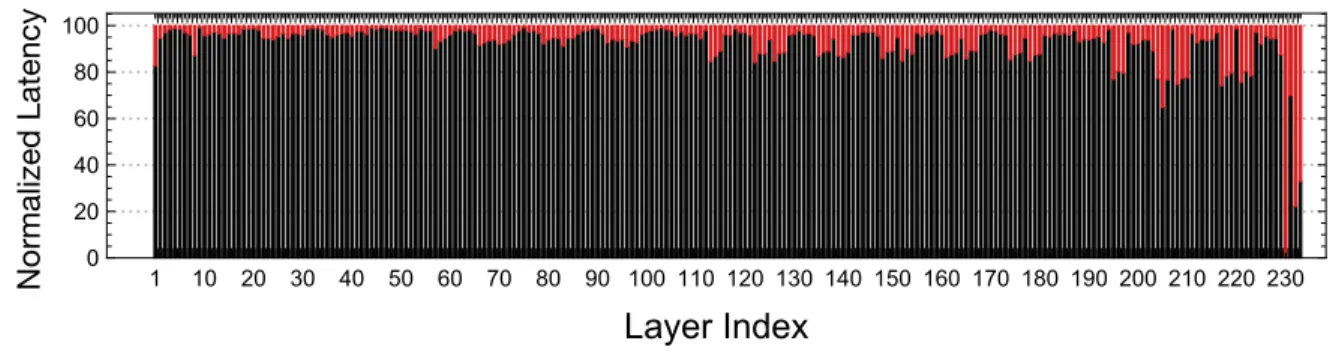
For each of the 50 models, we compare both sequential and parallel total layer latency to the model’s end-to-end latency. Figure 3.3 shows the normalized latencies in both cases. For models with parallel modules, the parallel total layer latencies are much lower than the model’s end-to-end latency. The difference between the sequential total layer latencies and the models’ end-to-end latencies are small. The normalized latencies are close to 1 with a geometric metric mean of 91.8% for the sequential case. This suggests the current software/hardware stack does not exploit parallel execution of data-independent layers or overlapping of layer execution, we verified this by inspecting the source code of popular frameworks such as MXNet, PyTorch, and TensorFlow.

(19)

��

Figure 3.3: The sequential and parallel total layer latency normalized to the model’s end-to-end latency using batch size 1 onc5.2xlargein Table 3.2.

The difference between a model’s end-to-end latency and its sequential total layer latency is due to the complexity of model execution within DL frameworks and the underlying software/hardware stack. We identified two major factors that may affect this difference: framework overhead and memory caching. Executing a model within frameworks introduced an overhead that is roughly proportional to the number of the layers. This is because frame-works need to perform bookkeeping, layer scheduling, and memory management for model execution. Therefore, the measured end-to-end performance can be larger than the total layer latency. On the other hand, both the framework and the underlying software/hard-ware stack can take advantage of caching to decrease the latency of data-dependent layers. For memory-bound layers, this can achieve significant speedup and therefore the measured end-to-end performance can be lower than the total layer latency. Depending on which fac-tor is dominant, the normalized latency can be larger or smaller than 1. Based on this, we formulate the 1 observation:

Observation 3.1: DL layers are the performance building blocks of the model perfor-mance, therefore, a model’s performance can be estimated using the performance of its layers. Moreover, a simple summation of layer-wise latency is an effective approximation of the end-to-end latency given the current DL software stack (no parallel execution of data-independent layers or overlapping of layer execution) on CPUs.

3.1.2 Layer Repeatability

From a model architecture point of view, a DL layer is identified by its type, shape, and parameters. For example, a convolution layer is identified by its input shape, output channels, kernel size, stride, padding, dilation, etc. Layers with the same type, shape, parameters (i.e. only differ in weights) are expected to have the same performance. We inspected the source code of popular frameworks and verified this, as they do not perform any special optimizations for weights. Thus in this paper we consider two layers to be the same if they have the same type, shape, parameters, ignoring weight values, and two layers are unique if they are not the same.

(20)

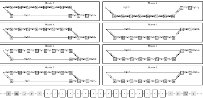
� BN P P P F S Module 1 Module 2 1 2 2 3 Module 3 Module 4 4 4 4 5 Module 5 Module 6 6 6 6 6 6 7 Module 7 Module 8 8 8 � � BN + BN � BN � BN 64 ⨯56 ⨯56 64⨯56⨯56 256⨯56⨯56 256⨯56⨯56 64⨯56⨯56 64⨯56⨯56 64⨯56⨯56 64⨯56⨯56 64⨯56⨯56 64⨯56⨯56 256⨯56⨯56 256 ⨯56 ⨯56 256⨯56⨯56 256⨯56⨯56 + � BN � BN � BN 256⨯56⨯56 256 ⨯₅₆ ⨯56 64⨯56⨯56 64⨯56⨯56 64⨯56⨯56 64⨯56⨯56 64⨯56⨯56 64⨯56⨯56 256⨯56⨯56 256⨯ 56⨯56 256⨯56⨯56 256⨯56⨯56 � � BN + BN � BN � BN 256 ⨯56 ⨯56 256⨯56⨯56 512⨯28⨯28 512⨯28⨯28 128⨯28⨯28 128⨯28⨯28 128⨯28⨯28 128⨯28⨯28 128⨯28⨯28 128⨯28⨯28 512⨯28⨯28 512 ⨯28 ⨯28 512⨯28⨯28 512⨯28⨯28 + � BN � BN � BN 512⨯28⨯28 512 ⨯₂₈ ⨯₂₈ 128⨯28⨯28 128⨯28⨯28 128⨯28⨯28 128⨯28⨯28 128⨯28⨯28 128⨯28⨯28 512⨯28⨯28 512⨯ 28⨯28 512⨯28⨯28 512⨯28⨯28 � � BN + BN � BN � BN 512 ⨯28 ⨯28 512⨯28⨯28 1024⨯14⨯14 1024⨯14⨯14 256⨯14⨯14 256⨯14⨯14 256⨯14⨯14 256⨯14⨯14 256⨯14⨯14 256⨯14⨯14 1024⨯14⨯14 1024 ⨯14 ⨯14 1024⨯14⨯141024⨯14⨯14 + � BN � BN � BN 1024⨯14⨯14 1024 ⨯14 ⨯14 256⨯14⨯14 256⨯14⨯14 256⨯14⨯14 256⨯14⨯14 256⨯14⨯14 256⨯14⨯14 1024⨯14⨯14 1024 ⨯14⨯14 1024⨯14⨯141024⨯14⨯14 � � BN + BN � BN � BN 1024 ⨯₁₄ ⨯₁₄ 1024⨯14⨯14 2048⨯7⨯7 2048⨯7⨯7 512⨯7⨯7 512⨯7⨯7 512⨯7⨯7 512⨯7⨯7 512⨯7⨯7 512⨯7⨯7 2048⨯7⨯7 2048 ⨯7⨯₇ 2048⨯7⨯7 2048⨯7⨯7 + � BN � BN � BN 2048⨯7⨯7 2048 ⨯7⨯₇ 512⨯7⨯7 512⨯7⨯7 512⨯7⨯7 512⨯7⨯7 512⨯7⨯7 512⨯7⨯7 2048⨯7⨯7 2048 ⨯7⨯7 2048⨯7⨯7 2048⨯7⨯7

Figure 3.4: The ResNet-50 (ID=14) architecture. The detailed ResNet modules 1−8 are listed above the model graph.

� � � � � � � � � _�� _�� _�� _�� _�� _�� _�� _�� _�� _�� _�� _�� _�� _�� _�� _�� _�� _�� _�� _�� _�� _�� _�� _�� _�� _�� _�� _�� _�� _�� _�� _�� _�� _�� _�� _�� _�� _�� _�� _�� _�� % ��

Figure 3.5: The percentage of unique layers in the models in Table 3.1, indicating that some layers are repeated within the model.

DL models tend to have repeated layers or modules (or subgraphs, e.g. Inception and ResNet modules). For example, Figure 3.4 shows the model architecture of ResNet-50 with the ResNet modules detailed. Different ResNet modules have layers in common and ResNet modules 2, 4, 6, 8 are entirely repeated within ResNet-50. Moreover, DL models are often built on top of existing models (e.g. transfer learning [17] where models are retrained with different data), using common modules (e.g. TensorFlow Hub [18]), or using layer bundles for Neural Architecture Search [19, 20]. This results in ample repeated layers when looking at a corpus of models. We quantitatively explore the layer repeatability within and across models.

Figure 3.5 shows the percentage of unique layers within each model in Table 3.1. We can see that layers are extensively repeated within DL models. For example, in Unguided

Volumetric Regression Net for 3D Face Reconstruction(ID=47) which has 1029

(21)

�� % ��

Figure 3.6: The type distribution of the repeated layers.

each model and Figure 3.6 shows their type distribution. As we can see Convolution, Ele-mentwise, BatchNorm, and Norm are the most repeated layer types in terms of intra-model layer repeatability. If we consider all 50 models in Table 3.1, the total number of layers is 10, 815, but only 1, 529 are unique (i.e. 14% are unique).

��

Figure 3.7: The Jaccard Similarity grid of the models in Table 3.1. Solid red indicates two models have identical layers, and black means there is no common layer.

We illustrate the layer repeatability across models by quantifying the similarity of any two models listed in Table 3.1. We use the Jaccard similarity coefficient; i.e. for any two models

M1 and M2 the Jaccard similarity coefficient is defined by

|L1∩L2|

(22)

layers ofM1 andM2 respectively. The results are shown in Figure 3.7. Each cell corresponds

to the Jaccard similarity coefficient between the models at the row and column. As shown, models that share the same base architecture but are retrained using different data (e.g.

CycleGAN*models with IDs 26−35 andInception V1* models with IDs 6−8) have many common layers. Layers are common across models within the same family (e.g. ResNet*) since they are built from the same set of modules (e.g. ResNet-50 is shown in Figure 3.4), or when solving the same task (e.g. the image classification task category). Based on this, we formulate the 2 observation:

Observation 3.2: Layers are repeated within and across DL models. This enables us to decrease the benchmarking time since only a representative set of layers need to be evaluated. The above two observations suggest that if we can decompose models into layers, and then take the union of them to produce a set of representative runnable networks, then benchmarking the representative runnable networks is sufficient to construct the performance of the input models. Since we only look at the representative set, the total runtime is less than running all models directly, thus DLBricks can be used to reduce benchmarking time. Since layer decomposition elides the input model topology, models can be private while their benchmarks can be public. The next section (Section 3.2) describes how we leverage these two observations to build a benchmark generator while having a workflow where one can construct a model’s performance based on the benchmarked layer performance. We further explore the design space of benchmark granularity and its effect on performance construction accuracy.

3.2 DESIGN

This section presents the design of DLBricks , a composable benchmark generation system for DL models. The design is motivated by the two observations discussed in Section 3.1. DLBricks explores not only layer level model composition, but also sequence level composi-tion where alayer sequence is a chain of layers. Thebenchmark granularity (G) specifies the maximum numbers of layers within any layer sequence in the output generated benchmarks.

G is introduced to account for the effects of model execution complexity (e.g. framework overhead and caching as discussed in Section 3.1.1). Thus, a largerGis expected to increase the accuracy of performance construction. On the other hand, a larger G might decrease the layer repeatability across models. Therefore, a balance needs to be struck (by the user) between performance construction accuracy and benchmarking time speedup.

(23)

{

P

_M 1

, …, P

Mn

}

Performance

Constructor

4

{

P

_S 1

, …, P

Sk

}

3

{

M

₁

, …, M

_n

}

{

S

₁

, …,

S

_k

}

Running Benchmarks

Benchmark

Generator

Benchmark

Granularity

1 1 2 6 5 §4.1 §4.2 Pe rf orma nce C on st ru ct io n W orkf lo w Be nch ma rk G en era tio n W orkf lo w Legend:

Figure 3.8: DLBricks design and workflow.

The design and workflow of DLBricks is shown in Figure 3.8. DLBricks consists of a benchmark generation workflow and a performance construction workflow. To generate composable benchmarks, one uses the benchmark generation workflow where: 1 the user inputs a set of models (M1, ...,Mn) along with a target benchmark granularity. 2 The

benchmark generator parses the input models into a representative (unique) set of non-overlapping layer sequences and then generates a set of runnable networks (S1, ...,Sk) using

these layer sequences’ information. 3 The user evaluates the set of runnable networks on a system of interest to get each benchmark’s corresponding performance (PS1, ...,PSk). The

benchmark results are stored and 4 are used within theperformance construction workflow.

5 To construct the performance of an input model, the performance constructor queries the stored benchmark results for the layer sequences within the model, and then 6 computes the model’s estimated performance (PM1, ...,PMk). This section describes both workflows in

(24)

3.2.1 Benchmark Generation

The benchmark generator takes a list of modelsM1,. . .,Mnand a benchmark granularity

G. Thebenchmark granularity specifies the maximum sequence length of the layer sequences generated. This means that whenG= 1, each generated benchmark is a single-layer network, whereas when G= 2 each generated benchmark contains at most 2 layers.

To split a model with the specified benchmark granularity, we use FindModelSubgraphs

(Algorithm 3.1). TheFindModelSubgraphs takes a model and a maximum sequence length and iteratively generates a set of non-overlapping layer sequences. First, the layers in the model are sorted topologically and then call the SplitModel function (Algorithm 3.2) with the desired begin and end layer offset. This SplitModel tries to create a runnable DL network (i.e., a valid DL network) using the range of layers desired, if it fails (e.g., a network which cannot be constructed due to input/output layer shape mismatch1_{), then}

SplitModel creates a network with the current layer and shifts the begin and end posi-tions. TheSplitModel returns a list of runnable DL networks (Si, . . . ,Si+j) along with the

end position to FindModelSubgraphs. The FindModelSubgraphs terminate when no other subsequences can be created.

Algorithm 3.1 The FindModelSubgraphs algorithm. Input: M (Model), G (Benchmark Granularity) Output: M odels

1: begin←0,M odels← {}

2: verts←TopologicalOrder(ToGraph(M))

3: while begin≤Length(verts)do

4: end←Min(begin+G,Length(vs))

5: sm←SplitModel(verts,begin,end)

6: M odels ←M odels+sm[“models”]

7: begin←sm[“end”] + 1

8: end whilereturnM odels

The benchmark generator applies theFindModelSubgraphs for each of the input models. A set of representative (i.e. unique) runnable DL networks (S1, . . . , Sk) is then computed.

We say two sequences S1 and S2 are the same if they have the same topology along with

the same node parameters (i.e. they are the same DL network modulo the weights). The unique networks are exported to the frameworks’ network format and the user runs them

1_{An example invalid network is one which contains a Concat layer, but does not have all of the Concat}

(25)

with synthetic input data based on each network’s input shape. The performance of each network is stored (PSi . . . , PSk) and used by the performance construction workflow.

Algorithm 3.2 The SplitModel algorithm. Input: verts, begin,end

Output: h“models”,“end”i .Hash table

1: vs←verts[begin:end]

2: m←CreateModel(vs) .Creates a valid model return

h“models”→ {m},“end” →endi .Hash table with keys: “model” and “end” ModelCreateException

3: m← {CreateModel({verts[begin]})} .Creates a model with a single node

4: n←SplitModel(verts,begin+ 1,end+ 1) . Recrusively split the model return

h“models”→m+n[“models”] ,“end” →n[“end”]i

3.2.2 DL Model Performance Construction

DLBricks uses the performance of the layer sequences to construct an estimate to the end-to-end performance of the input model M. To construct a performance estimate, the input model is parsed and goes through the same process 1 in the Figure 3.8. This creates a set of layer sequences. The performance of each layer sequence is queried from the bench-mark results (PSi, . . . , PSk). DLBricks supports both sequential and parallel performance

construction. Sequential performance construction is performed by summing up all the re-sulting queried results, whereas parallel performance construction sums up the results along the critical path of the model. Since current frameworks exhibit a sequential execution strat-egy (from Section 3.1.1), sequential performance construction is used within DLBricks by default. Other performance constructions can be easily added to DLBricks to accommodate different framework execution strategies.

3.3 EVALUATION

This section demonstrates that DLBricks is valid in terms of performance construction accuracy and benchmarking time speedup. We explore the effect of benchmark granularity on the constructed performance estimation as well as the benchmarking time. We evaluated DLBricks with 50 DL models (listed in Table 3.1) using MXNet (v1.5.1 using MKL v2019.3) on 4 different Amazon EC2 instances. These systems are recommended by Amazon [21]

(26)

Table 3.2: Evaluations are performed on the 4 Amazon EC2 systems listed. The c5.* systems operate at 3.0GHz, while thec4.*systems operate at 2.9GHz. The systems are ones recommended by Amazon for DL inference.

Instance CPUS Memory (GiB) $/hr

c5.xlarge 4 Intel Platinum 8124M 8GB 0.17

c5.2xlarge 8 Intel Platinum 8124M 16GB 0.34

c4.xlarge 4 Intel Xeon E5-2666 v3 7.5GB 0.199

c4.2xlarge 8 Intel Xeon E5-2666 v3 15GB 0.398

� � � � � � � � � _�� _�� _�� _�� _�� _�� _�� _�� _�� _�� _�� _�� _�� _�� _�� _�� _�� _�� _�� _�� _�� _�� _�� _�� _�� _�� _�� _�� _�� _�� _�� _�� _�� _�� _�� _�� _�� _�� _�� _�� _�� ( � )

Figure 3.9: The end-to-end latency of all models in log scale across systems.

for DL inference and are listed in Table 3.2. To maintain consistent CPU evaluation, the systems are configured to disable CPU frequency scaling, turbo-boosting, scaling-governor, and hyper-threading. Each benchmark is run 100 times and the 20th percentile trimmed mean is reported.

3.3.1 Performance Construction Accuracy

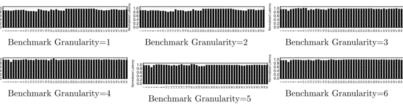
We first ran the end-to-end models on the 4 systems to understand their performance characteristics, as shown in Figure 3.9. Then, using DLBricks, we constructed the latency estimate of the models based on the performance of their layer sequence benchmarks. Figure 3.10 shows the constructed model latency normalized to the model’s end-to-end latency for

�� Benchmark Granularity=1 �� Benchmark Granularity=2 �� Benchmark Granularity=3 �� Benchmark Granularity=4 �� Benchmark Granularity=5 �� Benchmark Granularity=6

Figure 3.10: The constructed model latency normalized to the model’s end-to-end latency for the 50 model in Table 3.1 on c5.2xlarge. The benchmark granularity varies from 1 to 6. Sequence 1 means each benchmark has one layer (layer granularity).

(27)

all the models with varying benchmark granularity from 1 to 6 onc5.2xlarge. We see that the constructed latency is a tight estimate of the model’s actual performance across models and benchmark granularities. E.g., for benchmark granularityG= 1, the normalized latency ranges between 82.9% and 98.1% with a geometric mean of 91.8%.

As discussed in Section 3.1.1, the difference between a model’s end-to-end latency and its constructed latency is due to the combinational effect of model execution complexity such as framework overhead and caching, thus the normalized latency can be either below or above 1. For G = 1 (layer granularity model decomposition and construction), where a model is decomposed into the largest number of sequences, the constructed latency is slightly less accurate compared to other G values. Using the number of layers in Table 3.1 and the model end-to-end latency in Figure 3.9, we see no direct correlation between the performance construction accuracy, number of model layers, or end-to-end latency.

Figure 3.11 shows the geometric mean of the normalized latency (the constructed latency normalized to the end-to-end latency) of all the 50 models across systems and benchmark granularities. Model execution in a framework is system-dependent, thus the performance construction accuracy is not only model-dependent but also system-dependent. Overall, the estimated latency is within 5% (e.g.,G= 3, 5, 9, 10) to 11% (G= 1) of the model end-to-end latency across systems. This demonstrates that DLBricks provides a tight estimate to the input models’ actual performance across systems.

3.3.2 Benchmarking Time Reduction

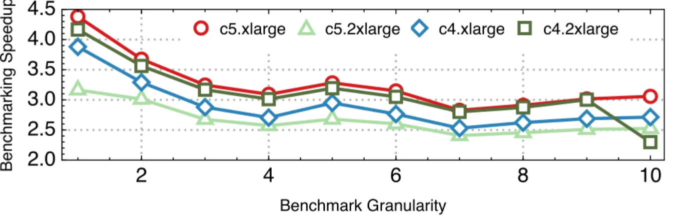
DLBricks decreases the benchmarking time by only evaluating the unique layer sequences within and across models. Recall from Section 3.1.2 that for all the 50 models, the total number of layers is 10, 815, but only 1, 529 are unique (i.e. 14% are unique). Figure 3.12 shows the speedup of the total benchmarking time across systems as benchmark granularity varies. The benchmarking time speedup is calculated as the sum of the end-to-end latency of all models divided by the sum of the latency of all the generated benchmarks. Up to 4.4× benchmarking time speedup is observed for G = 1 on the c5.xlarge system. The speedup decreases as the benchmark granularity increases. This is because as the benchmark granularity increases, the chance of having repeated layer sequences within and across models decreases.

Figure 3.11 and Figure 3.12 suggest a trade-off exists between the performance construc-tion accuracy and benchmarking time speedup and the trade-off is system-dependent. For example, while G = 1 (layer granularity model decomposition and construction) produces the maximum benchmarking time speedup, the constructed latency is slightly less accurate

(28)

��

�

��

Figure 3.11: The geometric mean of the normalized latency (constructed vs end-to-end latency) of all the 50 models on the 4 systems with varying benchmark granularity from 1 to 10.

��

�

��

Figure 3.12: The speedup of total benchmarking time for all the models across systems and bench-mark granularities.

comparing to otherG values on the systems. Since this accuracy loss is small, overallG= 1 is a good choice of benchmark granularity configuration for DLBricks given the current DL software stack on CPUs.

3.4 RELATED WORK

To characterize the performance of DL models, both industry and academia have invested in developing benchmark suites that characterize models and systems. The benchmarking methods are either end-to-end benchmarks (performing user-observable latency measurement on a set of representative DL models [3, 4, 6]) or are micro-benchmarks [4, 5, 22] (isolating common kernels or layers that are found in models of interest). The end-to-end benchmarks target end-users and measure the latency or throughput of a model under a specific workload scenario. The micro-benchmark approach, on the other hand, distills models to their basic atomic operations (such as dense matrix multiplies, convolutions, or communication

(29)

rou-tines) and measures their performance to guide hardware or software design improvements. While both approaches are valid and have their use cases, their benchmarks are manually selected and developed. As discussed, curating and maintaining these benchmarks requires significant effort and, in the case of lack of maintenance, these benchmarks become less representative of real-world models.

DLBricks complements the DL benchmarking landscape as it introduces a novel bench-marking methodology which reduces the effort of developing, maintaining, and running DL benchmarks. DLBricks relieves the pressure of selecting representative DL models and copes well with the fast-evolving pace of DL models. DLBricks automatically decomposes DL mod-els into runnable networks and generates micro-benchmarks based on these networks. Users can specify the benchmark granularity. At the two extremes, when the granularity is 1 a layer-based micro-benchmark is generated, whereas when the granularity is equal to the number of layers within the model then an end-to-end network is generated. To our knowl-edge, there has been no previous work solving the same problem and we are the first to propose such a design.

Previous work [23] also decomposed DL models into layers, but uses the results to guide performance optimization. DLBricks focuses on model performance and aims to reduce benchmarking effort. DLBricks shares similar spirit to synthetic benchmark generation [24]. However, to the authors’ knowledge, there has been no previous work on synthetic benchmark generation for DL.

3.5 DISCUSSION AND FUTURE WORK

Generating Overlapping Benchmarks — The current DLBricks design only considers non-overlapping layer sequences during benchmark generation. This may inhibit some types of optimizations (such as layer fusion). A solution requires a small tweak to Algorithm 3.1 where we increment the begin by 1 rather than the end index of theSplitModel algorithm (line 7). A small modification is also needed within the performance construction step to pick the layer sequence resulting in the smallest latency. Future work would explore the design space when the generated benchmarks can overlap.

Adapting to Framework Evolution — The current DLBricks design is based on the observation that current DL frameworks do not execute data-independent layers in parallel. Although DLBricks supports both sequential and parallel execution (assuming all data-independent layers are executed in parallel as described in Section 3.2.2), as DL frameworks start to have some support of parallel execution of data-independent layers, the current

(30)

design may need to be adjusted. To adapt DLBricks to this evolution of frameworks, one can adjust DLBricks to take user-specified parallel execution rules. DLBricks can then use the parallel execution rules to make a more accurate model performance estimation.

Sparse Models — The current DLBricks design assumes the input models are dense models. In a sparse model where the layers’ weights are sparse tensors2_{, the sparsity pattern}

(i.e., the distribution of non-zeros) of a layer’s weights affects the performance of the layer. To adapt DLBricks to sparse models, we need to consider the sparsity pattern of layer weights when identifying layers as performance building blocks (Section 3.1.1) or exploring their repeatability (Section 3.1.2). Recall that the sparsity of model layers is fixed in inference, we can use the sparsity pattern signature and encode it within the layer description. This would allow us to avoid unifying layers with different sparsity patterns and correctly reflect the sparsity effects and their influence on the layer performance. Future work would explore this encoding.

Other Systems — While this work focuses on CPUs, we expect the design to hold for GPUs and other AI chips. As stated in Observation 1 in Section 3.1.1, a simple summation of layer-wise latency is an effective approximation of the model’s end-to-end latency given the current DL software stack on CPUs. On GPUs and AI chips, a summation of layer-wise latency may no longer be effective due to the more aggressive DL optimizations done on these systems. Thus, to accommodate DLBricks to GPUs or AI chips, the execution strategy used in the benchmark generation and performance construction needs to be modified to reflect the DL model execution on those systems. Future work would explore the design for GPUs and other AI chips.

Other Use Cases — We are also interested in other use cases that are afforded by the DLBricks design — model/system comparison and advising for the cloud. For example, it is common to ask questions such as, given a DL model, which system should I use? or given a system and a task, which model should I use? Using DLBricks, system providers can curate a continuously updated database of the generated benchmarks results across different system offerings. The system providers can then perform a static performance estimate of the user’s DL model (without running it) and give suggestions as to which system to choose. This catalog of benchmark performance can also be shared to the public through secured APIs.

(31)

3.6 CONCLUSION

The fast-evolving landscape of DL poses considerable challenges in the DL benchmarking practice. While benchmark suites are under pressure to be agile, up-to-date, and repre-sentative, we take a different approach and propose a novel benchmarking design — aimed at relieving this pressure. Leveraging the key observations that layers are the performance building block of DL models and the layer repeatability within and across models, DLBricks automatically generates composable benchmarks that reduce the effort of developing, main-taining, and running DL benchmarks. Through the evaluation of state-of-the-art models on representative systems, we demonstrated that DLBricks provides a trade-off between performance construction accuracy and benchmarking time speedup. As the benchmark generation and performance construction workflows in DLBricks are fully automated, the generated benchmarks and their performance can be continuously updated and augmented as new models are introduced with minimal effort from the user. Thus DLBricks copes with the fast-evolving pace of DL models.

(32)

CHAPTER 4: XSP: UNDERSTANDING DL PERFORMANCE ACROSS STACK

This chapter proposes XSP — an across-stack profiling design that gives a holistic and hierarchical view of ML model execution. XSP leverages distributed tracing to aggregate and correlate profile data from different sources. XSP introduces a leveled and iterative measurement approach that accurately captures the latencies at all levels of the HW/SW stack in spite of the profiling overhead.

Machine learning/deep learning (ML) models are increasingly being used to solve problems across many domains such as image classification, object detection, machine translation, etc. This has resulted in a surge of interest in optimizing and deploying these models on many hardware types including commodity servers, accelerators, reconfigurable hardware, mobile/edge devices, and ASICs. As a result, there is an increasing need to profile and understand the performance of ML models.

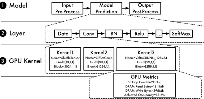
Characterizing ML model inference is complex as its performance depends on the interplay between different levels of the HW/SW stack — frameworks, system libraries, and hardware platforms. Figure 4.1 shows an example model inference pipeline on GPUs. At the top, there is the 1 model-level evaluation pipeline. Components at the model-level include input pre-processing, model prediction, and output post-processing. Within the model prediction step are the 2layer-level components — layer operators including convolution (Conv), batch normalization (BN), softmax, etc. Within each layer are the 3GPU kernel-level components — a sequence of CUDA API calls or GPU kernels invoked by the layer. Because of the complexities of model inference, one needs a holistic view of the execution to identify and locate performance bottlenecks.

Existing profiling tools or methods only provide a partial view of model execution. To capture a holistic view of model execution, one has to switch between an array of tools. Take the current ML profiling on GPUs for example. To measure the model-level latency, one inserts timing code around the model prediction step of the inference pipeline. To capture the layer-level information, one uses the ML framework’s profiling capabilities [25, 26]. And, to capture GPU kernel information, one uses GPU profilers such as NVIDIA’s nvprof [8] or Nsight [9]. The output profiles from the different tools are disjoint; e.g., the GPU kernels are not correlated with the layers. As a result, one cannot construct Figure 4.1 and identify that the three GPU kernels shown come from the first Conv layer, for example. This same issue exists when profiling ML model execution on CPUs.

(33)

instru-Input Pre-Process Output Post-Process Model Prediction … BN

Data Conv Relu SoftMax

Kernel1 Name=ShuffleTensor Grid= Kernel2 Name=OffsetComp Grid= Kernel3 Name=VoltaCUDNN_128x64 Grid= GPU Metrics SP Flop Count=62GFlop DRAM Read Bytes=12.1MB DRAM Write Bytes=296MB Achieved Occupancy=13.2%

Model

1

GPU Kernel

3

Layer

2

Figure 4.1: The model-, layer-, and GPU kernel-level profile of MLPerf ResNet50 v1.5(Table 4.8) onTesla V100(Table 4.7) with batch size 256 using NVIDIA GPU Cloud TensorFlow v19.06. The layers executed are data (Data), convolution (Conv), batch normalization (BN), relu (Relu), etc. The 3 GPU kernels from the first Conv layer are shown along with the GPU metrics of Kernel 3.

ment them to work with their profilers. For example, NVIDIA GPU Cloud [27] (NGC) hosts frameworks which are instrumented with NVTX [28] markers. The NVTX markers are added around each layer in the framework and are captured along with GPU events by Nvidia’s nvprof and Nsight profilers. However, this approach only annotates GPU kernel-level in-formation with layer names and lacks the layer-level profiling reported by the framework. Moreover, using these instrumented frameworks creates vendor lock-in — making the profil-ing and analysis dependent on the vendor’s frameworks and profilers. This is not an option for ML models developed or deployed using customized or non-vendor supported frameworks. To address the above issue, we propose XSP [29] — an across-stack profiling design along with a leveled experimentation methodology. XSP innovatively leverages distributed tracing to aggregate and correlate the profiles from different sources into a single timeline trace. Through the leveled experimentation methodology, XSP copes with the profiling overhead and accurately captures the profiles at each HW/SW stack level. Users can use XSP to have a smooth hierarchical step-through of model performance at different levels within the HW/SW stack and identify bottlenecks. Unlike existing approaches, XSP requires no framework modifications. We implement the profiling design for GPUs and couple it with an across-stack analysis pipeline. The analysis pipeline consumes the across-stack profiling trace and performs 15 types of automated analyses (Table 4.1). These analyses allow us to characterize ML models and their interplay with frameworks, libraries, and hardware. The

(34)

consistent profiling and automated analysis workflows in XSP enable systematic comparisons of models, frameworks, and hardware.

This chapter makes the following contributions:

• We propose XSP, an across-stack profiling design that innovatively leverages distributed tracing to aggregate profile data from different profiling sources and construct a holistic view of ML model execution.

• We introduce a leveled experimentation methodology that allows XSP to accurately cap-ture the profile at each HW/SW stack level despite the profiling overhead.

• We implement the design for GPU ML model inference and couple it with an analysis pipeline that performs 15 types of automated analyses to systematically characterize ML model execution.

• We conduct comprehensive experiments to show the utility of XSP. We use 65 state-of-the-art ML models from MLPerf Inference, AI-Matrix, and TensorFlow and MXNet model zoos. We evaluate the models on 5 representative systems that span the past 4 GPU generations (Turing, Volta, Pascal, and Maxwell) and present performance insights that would otherwise be difficult to discern absent XSP.

4.1 ML PROFILING ON GPUS AND RELATED WORK

Researchers leverage different tools and methods to profile ML model execution at each specific level of the HW/SW stack on GPUs. Figure 4.1 illustrates the model-, layer-, and GPU kernel-level profiling levels on GPUs.

1 Model-level profiling measures the steps within the model inference pipeline. There exist active efforts by both research and industry to develop benchmark suites [3, 4] to mea-sure and characterize models under different workload scenarios. For model-level profiling, researchers manually insert timing code around inference steps such as input pre-processing, model prediction, and output post-processing. Researchers then use the results as reference points to compare models or systems.

2 Layer-level profiling measures the layers executed by the ML framework using the framework’s profilers [25, 26]. These framework profilers are either built-in to the framework or are community-contributed framework plugins. The layer index, name, latency, and memory allocations are captured by the framework profiler as it is executing the layers. Researchers explicitly enable the framework’s profiler in their code to get the layer-level profile in a framework-specific format.

3GPU kernel-levelprofiling measures the low-level GPU information. Using NVIDIA’s nvprof and Nsight profilers, researchers capture the executed GPU kernels information such

(35)

as their name, latency and metrics. NVIDIA’s nvprof and Nsight profilers are built on top of the NVIDIA CUPTI library [30], which provides an API to capture CUDA API, GPU kernel, and GPU metric information.

The disconnect between the above profiling levels prohibits researchers from being able to have a holistic view of model execution — thus, limiting the types of analysis which can be performed. Take the MLPerf_ResNet50_v1.5model in Figure 4.1 for example. One can use the aforementioned profiling tools to get the most time-consuming layer (the 208th layer which is namedconv2d 48/Conv2D) and the most time-consuming GPU kernel (volta scudnn 128x64 relu interior nn v1). However, because of the lack of correlation between the GPU kernels and the layers, no other useful analysis can be performed. E.g, one can-not figure out the GPU kernels invoked by the most time-consuming layer, or correlate the most time-consuming GPU kernel to a specific layer within the model. Knowing the corre-lation between layers and GPU kernels enables more meaningful analyses and informs more optimization opportunities.

Currently, other than modifying framework source code, no tool or method exists to cor-relate the GPU kernel-level profile to the layer-level profile. For example, to be able to correlate GPU kernels to a certain layer, researchers manually instrument the framework’s source code with NVTX markers to annotate layers [31]. The NVTX markers are captured by the nvprof or Nsight profilers and kernels within the markers’ ranges belong to the anno-tated layers. Since the correlation between GPU kernels and layers is highly desired, NVIDIA provides modified versions of frameworks as Docker containers (NGC) where the frameworks are already instrumented with NVTX markers. While the profile captured in this approach correlates GPU kernels with layers, it lacks critical layer-level profiling (such as memory al-locations performed by a framework for a layer). Furthermore, current implementations [31] introduce barriers which inhibit frameworks from performing certain optimizations (such as layer-fusion) since the NVTX layer marking is performed by surrounding each layer with a “start NVTX marker” layer and an “end NVTX marker” layer. Finally, using vendor frameworks is not an option for profiling ML models developed with customized frameworks — a common practice when using user-defined layers.

To overcome the unknown correlation between layers and GPU kernels without vendor lock-in, there have been efforts [5, 22] to develop fine-grained micro-benchmarks of represen-tative layers. These micro-benchmarks target convolution or RNN layers and are purposely built for algorithm developers, compiler writers, and system researchers. Using layer param-eters of popular models, these micro-benchmark measure each layer in isolation. Thus, they do not reflect how layers are executed by frameworks. At best, micro-benchmarks give a lower-bound estimate of how layers would perform in an ideal scenario. This lower-bound

(36)

can be used to pinpoint potential optimizations in the HW/SW stack [23]. Recent bench-mark suites take a multi-tier approach [4, 7] and provide a collection