Basic Questions in Cluster Analysis

Cluster Analysis

Cluster analysis, like reduced space analysis (factor analysis), is concerned with data matrices in which the variables have not been partitioned beforehand into criterion versus predictor subsets. In reduced space analysis our interest centers on reducing the variable space to a smaller number of orthogonal dimensions, which maintains most of the information–metric or ordinal– contained in the original data matrix. Emphasis is placed on the variables rather than on the subjects (rows) of the data matrix. In contrast, cluster analysis is concerned with the similarity of the subjects–that is, the resemblance of their profiles over the whole set of variables. These variables may be the original set or may consist of a representation of them in reduced space (i.e., factor scores). In either case the objective of cluster analysis is to find similar groups of subjects, where “similarity” between each pair of subjects is usually construed to mean some global measure over the whole set of characteristics–either original variables or derived coordinates, if preceded by a reduced space analysis.

In this section we discuss various methods of clustering and the key role that distance functions play as measures of the proximity of pairs of points. We first discuss the fundamentals of cluster analysis in terms of major questions concerning choice of proximity measure, choice of clustering technique, and descriptive measures by which the resultant clusters can be defined. We show that clustering results can be sensitive to the type of distance function used to summarize proximity between pairs of profiles. We next discuss the characteristics of various computational algorithms that are used for grouping profiles, i.e., for partitioning the rows (subjects) of the data matrix. This is followed by brief discussions of statistics for defining clusters and the problems associated with statistical inference in this area.

The most common use of cluster analysis is classification. That is, subjects are separated into groups such that each subject is more similar to other subjects in its group than to subjects outside the group. Cluster analysis is thus con-cerned ultimately with classification and represents a set of techniques that are part of the field of numerical taxonomy (Frank and Green, [1968]; Punj and Stewart [1983]; Aldenderfer and Blashfield [1984]).

We will initially focus on clustering procedures that result in the assignment of each subject to one and only one class. Subjects within a class are usually assumed to be indistinguishable from one another. Thus, we assume that the underly-ing structure of the data involves an unordered set of discrete classes. In some cases we may also view these classes as hierarchical in nature, with some classes divided into subclasses.

Clustering procedures can be viewed as “pre-classificatory” in the sense that the researcher has not used prior judgment to partition the subjects (rows of the data matrix). However, it is assumed that some of the objectives are heterogeneous; that is, that “clusters” exist. This presupposition of different groups is based on commonalities within the set of indepen-dent variables. This assumption is different from that made in the case of discriminant analysis or automatic interaction

1 _{Nov 1, 2011 revision of Green, P.E., F. J. Carmone and S. M. Smith, Multidimensional Scaling, SECTION FIVE: DIMENSION REDUCING METHODS AND}

Basic Questions in Cluster Analysis

detection, where the dependent variable is used to formally define groups of objects and the distinction is not made on the basis of profile resemblance in the data matrix itself. Thus, given that no information on group definition is formally evaluated in advance, the major problems of cluster analysis will be discussed as follows:

1. What measure of inter-subject similarity is to be used and how is each variable to be “weighted” in the construction of such a summary measure?

2. After inter-subject similarities are obtained, how are the classes to be formed?

3. After the classes have been formed, what summary measures of each cluster are appropriate in a descriptive sense; that is, how are the clusters to be defined?

4. Assuming that adequate descriptions of the clusters can be obtained, what inferences can be drawn regarding their statistical significance?

The choice of proximity, similarity, association, or resemblance measure (all four terms will be used synonymously here) is an interesting problem in cluster analysis. The concept of similarity always connotes the question: similarity with respect to what? Proximity measures are usually viewed in relative terms–two objects are similar, relative to the group, if their profiles across variables are “close” or they share “many” aspects in common, relative to those which other pairs share in common. Most clustering procedures use pairwise measures of proximity. The choice of which subjects and variables to use in the first place is largely a matter for the researcher’s judgment. While these (prior) choices are important ones, they are beyond our scope of coverage. Even assuming that such choices have been made, however, the possible measures of pairwise proximity are many. Generally speaking, these measures fall into two classes: (a) distance-type measures (in-cluding correlation coefficients); and (b) matching-type measures. The characteristics of each class are discussed in turn.

A surprisingly large number of proximity measures–including correlation measures–can be viewed as distances in some type of metric space. In Section 2 we introduced the notion of Euclidean distance between two points in a space of r dimensions. We recall that the formula was:

where x_ij, x_jk are the projections of points i and j on dimension k; (k = 1,2,…,r). In as much as the variables are often mea-sured in different units, the above formula is usually applied after each variable has been standardized to mean zero and unit standard deviation. Our subsequent discussion will assume that this preliminary step has been taken. The Euclidean

Choice of Proximity Measure

distance measure assumes that the space of (standardized) variables is orthogonal, i.e., that the variables are uncor-related. While the Euclidean measure can still be used with correlated variables, it is useful to point out that (implicit) weighting of the components underlying the associated variables occurs with the use of the Euclidean measure:

1. Squared Euclidean distance in the original variable space has the effect of weighting each underlying principal component by that component’s eigenvalue.

2. Squared Euclidean distance in the component space (where all components are first standardized to unit variance) has the effect of assigning equal weights to all components.

3. In terms of the geometry of the configuration, in the first case all points are rotated to orthogonal axes with no change in squared inter-point distance. The general effect is to portray the original configuration as a hyper- ellipsoid with principal components serving as axes of that figure. Equating all axes to equal length has the effect of transforming the hyper-ellipsoid into a hyper-sphere where all “axes” are of equal length.

The above considerations can be represented in terms of the following squared distance model:

where: y_ik, y_jk denote unit variance components of profiles i and j on component axis k (k = 1,2,…,r). If one weights the component scores according to the variances of the components (before standardization) the expression is:

where is the k-th component variance, or eigenvalue. This expression is equivalent to d2

ij expressed in original variable

space. The above relationships assume that all principal components are extracted. As described earlier, if such is not the case, squared inter-point distances will be affected by the fact that they are computed in a component space of lower dimensionality than the original variable space. In summary, both the Euclidean distance measure in original vari-able space and the Euclidean distance in component space (assuming all components have been extracted) preserve all of the information in the original data matrix. Finally it should be pointed out that if (in addition to being standardized to mean zero and unit variance) the original variables are uncorrelated, both d2

ij and *d2ij will be equivalent.

Two other measures have often been proposed as proximity measures. Both of these measures derive from historical clus-tering methods, which used Q-type factor analysis to cluster subjects. In Q-type factor analysis–as described briefly in the Qualtrics White Paper on Factor Analysis–the correlation (or covariance) matrix to be factored consists of inter-subject rather than inter-variable proximities. In these methods the weights k are left intact.

Figures 1 and 2 show these effects geometrically. In the case of either covariance or correlation matrices the profile mean is subtracted from each vector component that, in the 2-component case of Figure 1, results in a centroid with an (new) origin located at point X on the figure. Figure 2 shows the effect of removing profile dispersion. If we assume that the pro-files were originally positioned in three-space, removal of each profile’s mean reduces their dimensionality to two-space. By using a correlation matrix we further reduce dimensionality by projecting all points on to the unit circle, since the dis-tance of the profile point can represent the standard deviation of a profile from the origin (the centroid of the points first having been translated to the origin). Thus, profiles a, b, and c would all be identical after the transformation, as would profiles d and e.

The cosine of the angle separating the two vectors represents the Q-correlation between them. Of course, there may be cases where the researcher is not interested in profile differences due to either mean and/or dispersion. If so, a Q-type analysis applied to covariance or correlation matrices, as the case may be, is perfectly sensible even though information is (willingly) discarded.

In general, we should expect differences in the derived squared distance measure computed from these procedures–both between themselves and between those computed by the techniques previously discussed. While the authors have a predi-lection for the information-preserving measures d2

ij and *d2ij, it is well to point out that no universally applicable distance

measure exists. The choice of which measure to use depends upon which aspect of the data is worth “preserving.” A wide variety of distance-type measures are available for cluster analysis; several of which are compared by Aldenderfer and Blashfield (1984). Once the researcher has selected a method of measuring pairwise profile similarity, the computa-tional routine for clustering the subjects must be selected. Aldenderfer and Blashfield identify several families of cluster-ing methods, each of which uses a different approach to creatcluster-ing groups: (1) hierarchical agglomerative; (2) hierarchical divisive; (3) factor analytic; (4) non-hierarchical.

These procedures are characterized by the construction of a hierarchy or tree-like structure. In some methods each point starts out as a unit (single-point) cluster. At the next level the two closest points are placed in a cluster. At the next level a third point joins the first two or else a second two-point cluster is formed, based on various criterion rules for assignment.

Figure  1      

Effect  of  Q-­‐type  Component  Analysis  on  Profile   Means  

Figure  2      

Effect  of  Q-­‐type  Component  Analysis  on  Profile   Dispersion

In application, hierarchical clustering is useful in determining if points are substitutable rather than mutually exclusive. The different assignment rules include:

SINGLE LINKAGE RULE

The single linkage or minimum distance rule starts out by finding the two points with the minimum distance. These are placed in the first cluster. At the next stage a third point joins the already-formed cluster of two if the minimum distance to any of the members of the cluster is smaller than the distance between the two closest unclustered points. Otherwise, the two closest unclustered points are placed in a cluster. The process continues until all points end up in one cluster. The distance between two clusters is defined as the shortest distance from a point in the first cluster that is closest to a point in the second.

COMPLETE LINKAGE RULE

The complete linkage option starts out in just the same way by clustering the two points with the minimum distance. However, the criterion for joining points to clusters or clusters to clusters involves maximum (rather than minimum) dis-tance. That is, a third point joins the already formed cluster of two if the maximum distance to any of the members of the cluster is smaller than the distance between the two closest unclustered points. In other words, the distance between two clusters is the longest distance from a point in the first cluster to a point in the second cluster.

AVERAGE LINKAGE

The average linkage option starts out in the same way as the other two. However, in this case the distance between two clusters is the average distance from points in the first cluster to points in the second cluster.

WARD’S METHOD

Ward’s Method starts out by finding two points with the minimum within groups sum of squares. Points continue to be joined to the first cluster or to other points depending on which combination minimizes the error sum of squares from the group centroid. This method is also known as a k-means approach. Closely related to Ward’s algorithm is the Howard-Harris algorithm [Howard-Harris, 1981]. The Howard-Howard-Harris algorithm is a hierarchical divisive method which uses the k-means method of assigning cases to the clusters. The k-means method assigns the case to the closest centroid. The approach may take either of the two forms described below:

K-MEANS APPROACH #1

1. Initially the entire set of observations is considered as one set. The group is split based on the one variable which makes the greatest contribution to within-group sum of squares.

would best improve the objective function is re-assigned. This process is repeated until a finite number of transfers are performed, no further improvement in within-groups sum of squares is found, or a local optimum is reached.

3. The group with the largest within-groups sum of squares is selected for splitting. Steps 2 and 3 are then repeated until the desired number of clusters is identified.

K-MEANS APPROACH #2

1. An m x m covariance matrix is formed and analyzed using principal components analysis. A factor score is computed for each of the n subjects on the first (and most important) dimension or factor.

2. All subjects with factor scores that exceed the mean value of the factor are assigned into a new cluster. 3. After splitting, each observation is re-evaluated against all clusters. If the objective function is improved by re-

assigning a case to another cluster, the case making the greatest improvement is re-assigned. Optimization continues until a) finite number of transfers are performed, b) no further improvement in the objective function is found, or c) a local optimum is reached.

4. The next factor is selected as the basis for splitting the next cluster. Steps 2, 3, and 4 are then repeated until the desired number of clusters is identified.

Hierarchical clustering algorithms may be identified as either hierarchical agglomerative or hierarchical divisive, mean-ing that they contract or expand the space between groups of points in the multivariate space. Divisive linkage methods tend to start new clusters rather than join points to existing clusters. Ward’s method and complete linkage rules are of the divisive variety and tend to create clusters of roughly equal size that are hyper-spherical in form. The average linkage method neither expands nor contracts the original space, while the single linkage tends to agglomerate or contract the space between groups of points in multivariate space.

FACTOR ANALYTIC METHODS FOR CLUSTERING

These methods analyze an n x n correlation matrix of similarities between the n cases to find a dimensional representa-tion of the points. Clusters are then developed based on the resulting factor loadings (the correlarepresenta-tion between the subject and the underlying dimension). Clustering using factor analytic methods has been criticized because of the use of a linear model that is developed across cases rather than across variables. The linear model tends to moderate the correct identification of anything other than linear additive predictive groups.

NON HIERARCHICAL METHODS FOR CLUSTERING

Non Hierarchical Methods have in general been subject to limited use and testing, making their specific operational characteristics difficult to identify. In general, however, these methods start right from a proximity matrix and work in the

1. Begin with an initial split of the data into a specified number of clusters. 2. Allocate each data point to the cluster with the nearest centroid.

3. Compute the new centroid of the clusters after all points are assigned to clusters. 4. Iterate steps 2 and 3 until no further changes occur.

Several general types of non-hierarchical clustering designs exist and can be characterized:

• SEQUENTIAL THRESHOLD–in this case a cluster center is selected and all objects within a pre-specified threshold

value are grouped. Then a new cluster center is selected and the process is completed. Once points enter a cluster they are removed from further processing.

• PARALLEL THRESHOLD–this method is similar to the one immediately above except that several cluster centers are

selected in advance and points within the threshold level are assigned to the nearest center; threshold levels can then be adjusted to admit fewer or more points to clusters.

• PARALLEL PARTITIONING–this method is similar to the one immediately above except that once several cluster

centers are chosen, the whole set of data is partitioned into disjoint sets based on nearest distance to cluster centers being within threshold distance of still other objects.

MATCHING-TYPE MEASURES

Quite often the analyst wishing to cluster profiles must contend with data that are only nominal scaled, in whole or in part. While dichotomous data, after suitable transformation, can often be expressed in terms of inter-point distances, the usual approach to nominal-scaled data uses attribute-matching coefficients. Intuitively speaking, two profiles are viewed as similar to the extent to which they share common attributes. As an illustration of this approach, consider the two profiles appearing below:

Each of the above objects is characterized by possession or non-possession of each of six attributes, where a “1" denotes possession and “0" denotes non-possession. Suppose we just count up the total number of matches –1, 1 or 0, 0– and divide by the total number of attributes. A simple matching measure could then be stated as:

S₁₂ = M/N = 2/6 = 1/3 where M denotes the number of attributes held in common (matching 1's or 0's) and N denotes the total number of attributes. We notice that this measure varies between zero and one. If weak matches (non-possession of an attribute) are to be de-emphasized, the above measures can be modified to:

No. of attributes that are 1 for both i and j

S

=

In this case, S_ij = 1/5. A variety of such matching type coefficients are described by Sneath and Sokal [1973] and Everett [1980]. Attributes need not be limited to dichotomies, however. In the case of unordered multichotomies, matching coef-ficients are often developed by means similar to the above by recoding the k-state variables into k-1 dummy (zero-one) variables. Naturally such coefficients will be sensitive to variation in the number of states in each multichotomy. Finally, mention should be made of the case in which the variables consist of mixed scales–nominal, ordinal, and inter-val. Interval-scaled variables may be handled in terms of similarity coefficients by the simple device of computing the range of the variable R_k and finding:

Gower (1967) suggested this measure as a means of handling both nominal- and interval-scaled data in a single simi-larity coefficient. Mixed scales, which include ordinal-scaled variables, present greater difficulties. If ordinal and interval scales occur, one can downgrade the interval-scaled data to ordinal scales and use nonmetric procedures. If all three scales–nominal, ordinal, and interval–appear, one is more or less forced to downgrade all data to nominal measures and use matching type coefficients.

An alternative approach would be to compute “distances” for each pair of objects according to each scale type sepa-rately, standardize the measures to zero mean and unit standard deviation, and then compute some type of weighted association measure. Such approaches are quite ad hoc, however. While the above classes of clustering algorithms are not exhaustive of the field, most of the currently available routines can be typed as falling into one (or a combination) of the above categories.

Criteria for grouping include such measures as average within-cluster distance and threshold cut-off values. The fact remains, however, that even the “optimizing” approaches generally achieve only conditional optima, since an unsettled question in this field is how many clusters to form in the first place.

The recommendation of an algorithm is difficult at best. For classification purposes, clusters should be able to identify distinct separations between different clusters of items. Clusters should also be internally consistent. Because meeting these challenges is often a function of the type of data analyzed, selection of an optimal algorithm is also a function of the characteristics of the data.

Overall, the k-means clustering technique appears to perform well (see Punj and Stewart 1983) when the initial starting configuration is non-random. In situations where a random starting configuration is required, the minimum variance type of algorithm often performs well. It is even suggested that clustering might best be approached using a combination of reduced space analysis and clustering techniques, so as to group points in the space obtained from principal components or nonmetric scaling techniques. This approach is particularly beneficial if the number of dimensions is small, allowing the researcher to augment the clustering results with visual inspection of the configuration. If the researcher is more concerned with structure than classification, overlapping clustering ignores the concept of distinct separations between clusters in an attempt to allow products/subjects to belong to more than one cluster.

DESCRIBING THE CLUSTERS

Once clusters are developed, the researcher still faces the task of describing the clusters. One frequently used measure is the centroid; that is, the average value of the objects contained in the cluster on each of the variables making up each object’s profile. If the data are interval scaled and clustering is performed in original variable space, this measure ap-pears quite natural as a summary description.

If the space consists of principal components’ dimensions obtained from nonmetric scaling methods, the axes usually are not capable of being described simply. Often in this case the researcher will want to go back to the original variables and compute average profile measures in these terms. If matching type coefficients are used, the cluster may be described by the group’s modal profile on each of the attributes; in other cases, arithmetic averages may be computed. In addition to central tendency, the researcher may compute some measure of the cluster’s variability, e.g., average inter-point distance of all members of the cluster from their centroid or average inter-point distance between all pairs of points within the cluster.

STATISTICAL SIGNIFICANCE

Despite attempts made to construct various tests of statistical significance of clusters, current statistical tests are little more than heuristics offering relatively indefensible procedures. The lack of appropriate tests stems from the difficulty of specifying realistic null hypotheses. First, it is not clear just what the universe of content is. Quite often the researcher arbitrarily selects objects and variables and is often interested in confining attention to only this sample. Second, the researcher is usually assuming that heterogeneity exists in the first place–otherwise, why bother to cluster? Moreover, the clusters are formed from the data and not on the basis of outside criteria. Thus, one would be placed in the uncomfort-able statistical position of “testing” the significance between groups formed on the basis of the data itself. Third, the distributions of objects are largely unknown, and it would be dangerous to assume that they conformed to some tractable model like a multivariate normal distribution. It is indeed likely that different types of clusters may be present simultane-ously in the data.

It is a major difficulty to specify a-priori the type of clustering or homogeneity to be detected. These limitations in mind, Arnold (1979) proposed using a statistic originally suggested by Friedman and Rubin (1967). The statistic, given by

where

| T | is the determinant of the total variance-covariance matrix | W | is the determinant of the pooled within-groups covariance matrix

We continue to believe that, at least in the present state of cluster analysis, the objective of this class of techniques should be to formulate rather than test categorizations of data. After a classification has been developed and supported by theoretical research and subsequent reformulation of classes, other techniques like discriminant analysis might prove

C = log max | T | | W |

useful in the assignment of new members to groups identified on grounds which are not solely restricted to the original cluster analysis.

While the above caveats are not to be taken lightly, clustering techniques are useful–in ways comparable to the objec-tives of factor analysis–as systematic procedures for the orderly preclassification of multivariate data. The results of using these approaches can be helpful and meaningful (after the fact) as will be illustrated next.

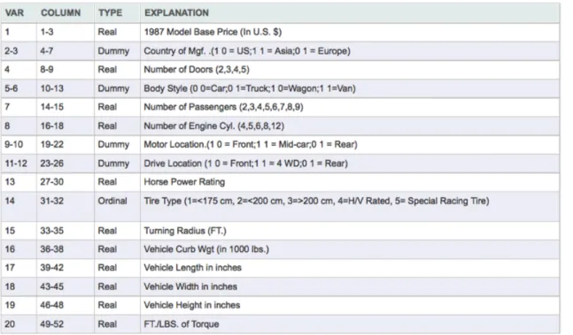
Thus far, our descriptions of reduced space and clustering methods have largely remained at the conceptual level. In this section of the section we describe their application to a realistically sized problem–one dealing with the similarities and differences among 90 1987 automobiles, trucks and utility vehicles whose prices range from $5,000 to $168,000. In this abridged version of the study, we illustrate the use of cluster analysis to 90 vehicles. Table 1 identifies the 20 attributes upon which data was collected for the 90 vehicles identified in Table 2. This 90 vehicle x 20 variable data matrix forms the basis for our analysis directed at grouping the vehicles according to similarity of attributes.

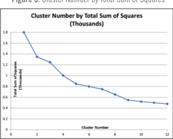
Application of the Howard Harris procedure yielded two different clustering solutions which, based on the within-group sum of squares for each group, appeared to be worth examining. Figure 3 shows the “Scree”-type diagram plotting sum of squares against number of clusters. The curve appears to flatten at 5 clusters and again at 12 clusters. The 5-cluster solution is shown in Table 3 and the 12-cluster solution is shown in Table 4. As might be surmised, the 5-cluster repre-sentation was inferior to the 12-cluster reprerepre-sentation.

An Application of

Reduced Space and Cluster Analysis

Table 1:

Vehicle Performance Characteristics and Listing

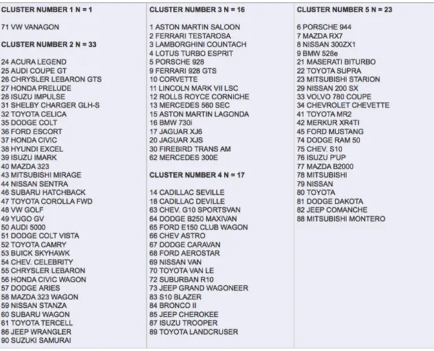
Table 3:

The Five-Cluster Solution

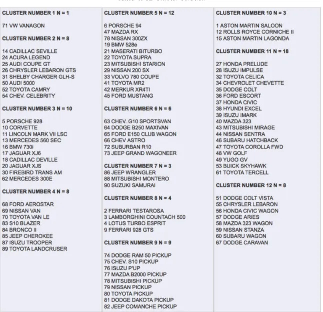
In Table 1, we note that cluster membership is somewhat more evenly distributed than in Table 2 (twelve) clusters. The groups are rather homogeneous, though now and again, a vehicle seems to be out of place. From Tables 1 and 2 one can get some idea of the current inter-manufacturer competition. Market positioning strategies seem to be well developed, with several of the manufacturers having multiple vehicles within the same segments. This product positioning is even more apparent when one recognizes that these are the major model differences and that minor options/product distinc-tions are present for most vehicles.

Table 4:

12-Cluster Solution

SUMMARY OF STUDY

The foregoing results constituted only one of several possible facets of this study. Additional analytical steps may have involved: (a) the development of clusters based only on the nominal-scaled (features) data; (b) the development of clusters based only on the interval-scaled data; and (c) clustering (involving both features and measured data) on a combined time period basis.

Other Considerations

in Clustering Techniques

In terms of substantive results, we found that five “clusters” explained most of the similarities and differences among the vehicles models–VW Vanagon, smaller 4-5 passenger vehicles and wagons, exotic sports and large capacity passen-ger cars and utility vehicles, and popular sports cars and pickups. Of course, the clusters became more detailed as the number of clusters increased.

The resulting clusters indicate which manufacturers compete with which other manufacturers in terms of similarity in the performance profiles of their vehicles. For purposes of this section, suffice it to say that clustering techniques can be used in marketing studies involving large-scale data banks. Moreover, the combination of reduced space (principal components) and cluster analysis can provide a useful dual treatment of the data. The reduced space phase may provide help in summarizing the original variables in terms of a smaller number of dimensions, e.g., speed or cargo capacity. The clustering phase permits one to group vehicles according to their coordinates in this reduced space.

Our previous discussion of clustering analysis has tended to emphasize the tandem approach of dimensional and nominal (class-like) representation of data structures. In addition to using multidimensional scaling techniques for reduced space analysis, a number of other nonlinear approaches have been developed, including nonlinear factor analysis [McDonald, 1962], polynomial factor analysis [Carroll 1969], correspondence analysis [Carroll, Green and Schaffer, 1986]. Space does not permit anything but brief mention of this interesting work. We do consider in some detail, however, a combina-tion qualitative-quantitative approach to an important problem in reduced space analysis–the interpretacombina-tion of data structures.

NOMINAL VS. DIMENSIONAL STRUCTURES

As mentioned earlier, even a pure class structure–where class membership accounts for all of the information in the data–can be represented spatially. More commonly, however, we consider cluster analysis as a more appropriate tech-nique for characterizing such data. On the other hand, other data structures are inherently dimensional, so that measures of proximity are assumed to be able to vary rather continuously throughout the whole matrix of proximities. Pure typal and pure dimensional structures represent only two extremes. Since all proximity matrices (that obey certain properties [Gower, 1966]) can be represented spatially, it would seem of interest to consider data structures in terms of the restrictions placed on the points as they are arranged in that space. This motivation underlies many of the developments in cluster analysis. Torgerson [1965] was one of the first researchers to become interested in the problem of characterizing data as “mixtures” of discrete class and quantitative variables. Several varieties of such structures can be obtained:

1. Data consisting of pure and unordered class structure. Dimensional representation of such data would consist of points at the n vertices of an n-1 dimensional simplex where inter-point distances are all equal. For example, three classes could be represented by an equilateral triangle in two-space, four classes by a regular

tetrahedron in three-space, and so on.

2. Data consisting of concentrated masses of points, corresponding to classes, where interclass distances are unequal, thus implying the existence of latent dimensions underlying class descriptions.

3. Data consisting of hierarchical sets of attributes where some classes are nested within other classes, e.g., cola and non-cola drinks within the diet-drink class.

4. Data consisting of dimensional variables nested within discrete classes, e.g., sweet to non-sweet cereals within the class of “processed” shape (as opposed to “natural” shape) cereals.

5. Data consisting of mixtures of ideal (mutually exclusive) classes so that one may find, for example, points in the interior of an equilateral triangle whose vertices represent three unordered classes.

6. Data consisting of pure dimensional structure in which, theoretically, all of the space can be filled up by points. While the above categorizations are neither exclusive nor exhaustive, they are illustrative of the variety of data struc-tures that could be obtained in the analysis of “objective” data or subjective (similarities) data of the sort described in the preceding sections. From the viewpoint of cluster analysis, some of the above structures could produce elongated, parallel clusters in which average intra-cluster distance need not be smaller than inter-cluster distances. Moreover, one could have structures in which the clusters curve or twist around one another along some manifold embedded in a higher dimensional space [Shepard and Carroll, 1966].

Figure 3 shows three types of data structures as related to the above categories [Torgerson, 1965]. The first panel illustrates the case of three unordered discrete classes. The second panel illustrates the case of discrete class structure where class descrip-tors are assumed to be orderable. The third panel shows the case of three discrete classes and an orthogonal variable, which is quantitative. Points oc-cur only along the solid lines of the prism. The fourth panel illustrates the case where objects are made up of mixtures of discrete classes plus an orthogonal quantitative dimension. In this case all objects lie on or within the boundaries of the curve prism while “pure” cases would lie at one of the three edges with location dependent upon the degree of the quantita-tive variable which each possesses.

Research in cluster analysis and related techniques is proceeding in new directions for dealing with heretofore-intractable data structures. The continued development and refinement of interactive display devices should further these efforts by enabling the researcher to “visualize” various characteristics of the data array as a guide to the selection of appropriate grouping methods

OVERLAPPING CLUSTERING TECHNIQUES

The key element of all clustering techniques discussed so far is the mutually exclusive and exhaustive nature of the clusters developed. While in most cases, managers view segments as mutually exclusive and hierarchical in nature, cases do exist where segments are mutually exclusive. Indeed, consumers may well fit into several segments. Overlapping clustering relaxes the exclusivity constraint of most other hierarchical and non-hierarchical cluster models. As an example of a cluster analysis of brands of soft drinks, Tab may be perceived as fitting into clusters identifying diet drink, cola, and used by women, whereas Diet Pepsi would fit into only the first two benefit clusters. Brands might compete across product categories. V8 drink would compete against other vegetable/fruit drinks, as well as against soft drinks and even as a between meals snack. A cluster of toothpaste users might show that Aqua-Fresh toothpaste appeals to the fresh breath, decay prevention, and brighteners clusters, while Crest may appeal to only the decay prevention benefit cluster. Overlap-ping clustering simply allows for patterns of overlapOverlap-ping to be considered.

Arabie [1977], Shepard and Arabie [1979], Arabie and Carroll [1980], Arabie, Carroll, DeSarbo and Wind [1981] outline methods for overlapping clustering, but point out that limitations do occur in practice. First, it is difficult to develop an algorithm that effectively considers all possible cluster overlap options, especially if the sample size is large. Second, most overlapping clustering algorithms produce too many clusters with excessive overlap. A high degree of overlap results in poor configuration recovery, or in other words, a great mathematical model that is difficult to visualize from the data. Shepard and Arabie [1979] provide a detailed explanation of their ADCLUS (for “additive clustering”) model. The ADCLUS model represents a set of m clusters which may or may not be overlapping. Each cluster is assigned a numerical weight, wk, where k=1,…,m. The similarity between any pair of points is predicted in the model as the sum of the weights of those clusters that contain the pair.

Arabie and Carroll [1980] and Arabie, Carroll, DeSarbo and Wind [1981] further develop the ability to fit the ADCLUS by presenting the MAPCLUS (for MAthematical Programming CLUStering) algorithm. This implementation appears to meet the needs of clustering items in more than a single cluster. In addition, clusters may be added, deleted, or modified to produce constrained solutions [Carroll and Arabie, 1980], and estimate (in a regression sense) the importance of new sets of clusters in explaining variance in the data.

The importance of overlapping clustering is self evident, particularly in applications where clusters are not mutually exclusive, but are overlapping. This reality reflects the existence of multi-attribute decision rules in decision-making behavior, divergent product application or use scenarios, and even joint decisions made by multiple users within the same household.

We’re Here to Help!

Qualtrics.com provides the most advanced online survey building, data col-lection (via panels or corporate / personal contacts), real-time view of survey results, and advanced “dashboard reporting tools”.

If you are interested in learning more about how the Qualtrics professional services team can help you with a conjoint analysis research project, contact us at [email protected].

Summary

This paper has considered a companion objective of the scaling of similarities and preference data–the use of metric and nonmetric approaches in data reduction and taxonomy. Clustering procedures are a helpful tool in data analysis when one desires to group objects (or variables) according to their relative similarity. We first provided a description of clustering methods and addressed the topics of association measures, grouping algorithms, cluster descriptions and statisti-cal inference. This led to presentation of some pilot research utilizing cluster analysis, in examining the performance structure of the automobile market. We concluded the section with a description of the general problem of portraying data structures that consist of mixtures of categorical and dimensional variables and a discussion of the usefulness of overlapping clustering.

1. We note that factor analysis can be used to cluster respondents and cluster analysis can be used to group variables. This is done by transposing the data matrix (i.e., using a variable by subject data matrix rather than the more common subjects by variables data matrix).