A Modified Approach to Identifying Multiple Outliers in
Multivariate Data
Benony Kwaku Gordor
Department of Computer Science, Ashesi University, 1 University, Avenue, Berekuso, PMB
CT 3 Cantonments, Accra, Ghana
E-mail of the corresponding author: [email protected]
Abstract
Using the likelihood-based Wilks’ method to identify multiple outliers in multivariate datasets can be computationally intensive. For example, to identify the most extreme k outliers in a sample of size n, the likelihood principle requires that we examine all
k n
subsets of observations. Faced with this amount of
computation, it seems reasonable to suggest that one examines only observations that lie at the periphery of the data ‘cloud’ rather than all the observations. However, this ‘short-cut’ approach raises two major questions. The first is how many observations at the periphery one has to examine and second, what the guarantee is that the observations that are identified are truly the outliers. This paper is an attempt to provide answers to these questions by conducting a simulation study involving a large number of datasets of various sizes, dimensions and degree of outlier contamination. In the end, a formula for identifying multiple outliers based on the approach is developed.
Key words: Outliers, Mahalanobis Distance, Optimal Subset, Failure Rate, Risk Table
1. Introduction
Practical problems in the identification of multiple outliers in multivariate datasets usually make use of the Wilks’ ratio statistic given by
, ) ( S S k T T R (1)
which determines the subset Tk of k observations among the sample of size n for which the ratio is minimum, where S is the sum of squares and cross-product matrix, and S(Tk) is the corresponding matrix with the
observations in Tk removed from the sample. The problem also uses any other method based on the likelihood ratio principle. This principle requires a two-stage approach to outlier identification. The principle as constructed by Barnett (1979) states that given a basic model, F, and an alternative contaminating model, F’, the most extreme observation is that one, xi, whose assignment as the contaminant in the sense of F’ maximizes the difference between the log-likelihoods of the sample under F’ and F. If this difference is surprisingly large, declare xi to be an outlier. The main concern in this paper is the application of the first stage of this principle because of the computational difficulties involved.
subset of size k maximizes the log-likelihood under F. This means that in a sample of size n, we must evaluate the log-likelihood for
k n
subsets. If we use the Wilks’ ratio method, for example, it means that we must
calculate k n
k-outlier scatter-ratios and examine them for extremeness. In large multi-dimensional datasets, this can be computationally prohibitive, even for a moderate value of k. For example, for even n40 and
, 2
k there are 780 ratios to examine; and for n50 and k3, there are 19,600 such ratios to examine. It is obviously prohibitive to examine all of these ratios.
In univariate data, we could order the n observations as x(1)x(2)x(n), so that the most outlying k-tuple is clearly a subset of the first few elements on either side. We may, for example, choose this subset to contain the lowest k and the highest k values:
) ( ) 1 ( ) ( ) ( ) 2 ( ) 1 ( x xk ,xn ,xn , ,xn k x , so we need to examine at most
k k 2
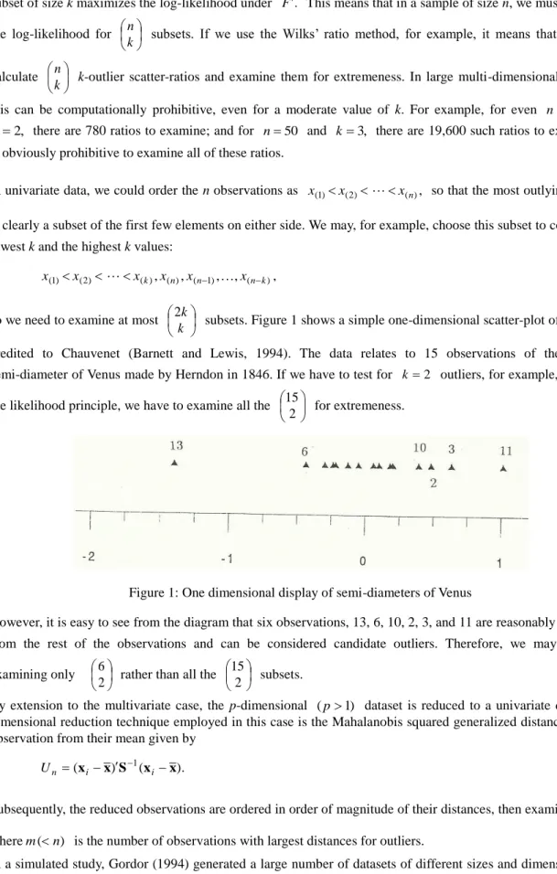
subsets. Figure 1 shows a simple one-dimensional scatter-plot of a dataset
credited to Chauvenet (Barnett and Lewis, 1994). The data relates to 15 observations of the vertical semi-diameter of Venus made by Herndon in 1846. If we have to test for k 2 outliers, for example, based on the likelihood principle, we have to examine all the
2 15 for extremeness.
Figure 1: One dimensional display of semi-diameters of Venus
However, it is easy to see from the diagram that six observations, 13, 6, 10, 2, 3, and 11 are reasonably separated from the rest of the observations and can be considered candidate outliers. Therefore, we may consider
examining only 2 6
rather than all the 2 15 subsets.
By extension to the multivariate case, the p-dimensional (p1) dataset is reduced to a univariate dataset. A dimensional reduction technique employed in this case is the Mahalanobis squared generalized distance of each observation from their mean given by
). ( ) (x x S 1 x x i i n U (2)
Subsequently, the reduced observations are ordered in order of magnitude of their distances, then examine k m ,
wherem(n) is the number of observations with largest distances for outliers.
In a simulated study, Gordor (1994) generated a large number of datasets of different sizes and dimensions. For each dataset, he calculated a failure rate, which he defined as the number of times that mk observations with
providing that the sample size is reasonably large (n30), failure rate is only weakly affected by the dimension of the data. The objective of this paper is to determine the number of observations, mk, such that examining only k mk
results in the k outliers being identified with 0% failure rate. We call this the optimum subset of extreme points.
2. Method
In this paper we shall determine the optimum subset for k1,2,3 and 4 extreme points or outliers. This work is limited to a maximum of 4, with the understanding that extreme values beyond 4 may not strictly be a problem of outlier identification but a discrimination between (two) groups. Given that failure rate is only weakly affected by the dimension of the data for large (n30) sample size, we generated a sample of size n50 and dimensionality of p4 in each case.
2.1 Unknown Number of Outliers
For this purpose, 100 datasets are generated each according to the following rules: With probability 0.9, sample
from Np(0,1) and with probability 0.1, sample from Np(c,1). Computationally, this means we generate x
from Np(0,1) and generate u from the uniform distribution U(0,1). If u0.9, we add c to x; if ,
9 . 0
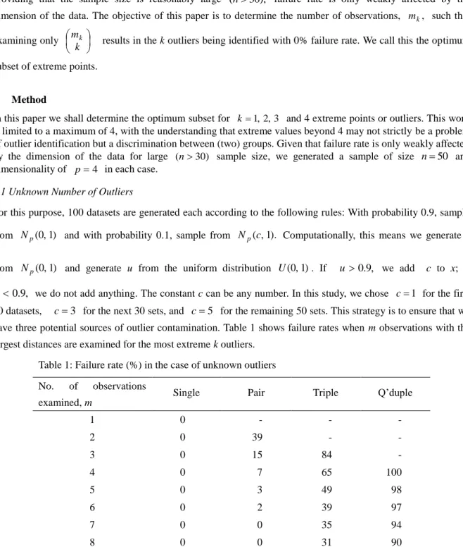
u we do not add anything. The constant c can be any number. In this study, we chose c1 for the first 20 datasets, c3 for the next 30 sets, and c5 for the remaining 50 sets. This strategy is to ensure that we have three potential sources of outlier contamination. Table 1 shows failure rates when m observations with the largest distances are examined for the most extreme k outliers.
Table 1: Failure rate (%) in the case of unknown outliers
No. of observations examined, m
Single Pair Triple Q’duple
1 0 - - - 2 0 39 - - 3 0 15 84 - 4 0 7 65 100 5 0 3 49 98 6 0 2 39 97 7 0 0 35 94 8 0 0 31 90
2.2 Two Known Outliers in Each Dataset
Dataset of size 50 are generated from N4(0,1) as before. Then we introduced two discordant outliers by adding two suitably chosen constants randomly to two of each of the 50 observations. (Two outliers are judged
discordant at 5% significant level when their Wilks’ ratio r2 is such that r2 0.688. The process was
repeated until 100 datasets, each contaminated with two discordant outliers, were obtained. Table 2 shows failure rates when m observations with the largest distances are examined for the most extreme k outliers.
Table 2: Failure rate (%) for a pair of outliers
No. of observations examined, m 2 3 4
Failure rate (%) 3 1 0
It can be observed from the table that in 3% of the samples, the process fails to identify the two outliers. In other words, failure rate for samples contaminated with two outliers is 3% when we limit the search to the two most extreme values; and if we extend the search for these outliers to three most extreme values, the failure rate falls to 1%. Finally, when the search for the outliers is extended to four most outlying observations, the failure rate is absolutely 0%. We can therefore conclude that to identify two outliers in a dataset, it is safe to search for them among the four most extreme observations only. Computationally, it means we need to search for a pair of
outliers by examining only 6 2 4
most extreme observations.
2.3 Three Known Outliers in each Dataset
We again generated data sets of size 50 each from N4(0,1) as before. Then we introduced three discordant outliers by adding three suitably chosen constants randomly to three of each of the 50 observations. The process was repeated until 100 datasets, each contaminated with three discordant outliers, were obtained. Table 3 shows failure rates when m observations with the largest distances are examined for the most extreme k outliers.
Table 3: Failure rate (%) for triple outliers
No. of observations examined, m 3 4 5 6 7
Failure rate (%) 46 20 3 1 0
It can be observed from the table that in 46% of the samples, the process fails to identify the three outliers. In other words, failure rate for samples contaminated with three outliers is 46% when we limit the search to the three most extreme values; and if we extend the search for these outliers to four most extreme values, the failure rate falls to 20%. Finally, when the search for the outliers is extended to seven most outlying observations, the failure rate is absolutely 0%. We can therefore conclude that to identify thee outliers in a data set, it is safe to search for them among the seven most extreme observations only. Computationally, it means we need to search
for a triple of outliers by examining only 35 3 7
most extreme observations.
2.4 Three Known Outliers in each Dataset
A similar simulation study shows (Table 4) that in the case of four outliers, we need to search among the nine most extreme observations.
Table 4: Failure rate (%) for quadruple outliers
No. of observations examined, m 4 5 6 7 8 9
Failure rate (%) 91 63 30 16 8 0
3. Results and Discussion
3.1 Optimum Number of Extreme Observations to Examine for Outliers
The results of the simulation exercise displaced in Tables 1 to 4 are summarized in Table 5. We refer to this table as ‘Risk Table’ for identifying multiple outliers in a multivariate data set. In the table, the figures represent failre rates when m observations with the largest Mahalanobis squared distances are examined for k-tuple (k = 1, 2, 3, 4) outliers.
Table 5: Risk table for finding multiple outliers in multivariate data
No. of outliers, k
No. of observations examined, mk
1 2 3 4 5 6 7 8 9
1 0 0 0 0 0 0 0 0 0
2 - 3 1 0 0 0 0 0 0
3 - - 46 20 3 1 0 0 0
4 - - - 91 63 30 16 8 0
From the table, it can be observed that the optimum number, mk, of most extreme observations that guarantees the correct choice of two discordant outliers is 4; that for three outliers is 7; and that for four outliers is 9. A striking relationship between mk,and k is now clear. This is,
2 , 1 2 2 , 2 k k k k mk
The relationship above therefore provides the following simple rule for identifying multiple outliers in multivariate datasets. The rule states that:
To find the k-tuple of discordant outliers in a multivariate dataset, one needs to examine at most 2k1 most extreme observations, as ordered by their generalized squared distances.
3.2 Comparing Results with Wilks’ Ratio Method
We now find it appropriate to compare our modified method with the well-known Wilks’ method of identifying outliers in multivariate data sets. Note that in the case of Wilks, the outliers are identified by examining all the
k n
outlier ratios rather than ,
k mk where mk n.
The data used are the well-known Iris Setosa data (Anderson, 2003) and the Transportation Cost data (Johnson & Wichern, 2002). We used these datasets because they are well-used in the literature (Wilks, 1963; Hadi, 1992; Caroni & Prescott, 1992; Nkansah & Gordor, 2012a; 2012b; 2013) on the study of outliers. The outliers identified in each case are shown in Table 6.
Table 6: Identifying Outliers in Iris Data using Wilks Ratio and Modified Method
Dataset
No. of outliers, k
Observations selected by the Wilks’ Ratio Method Modified Method
Iris Setosa 1 42 44 2 42 23 44 42 3 42 44 23 44 42 23 Transportation Cost 1 9 9 2 9 21 19 21 3 9 21 36 9 21 36
It can be observed from the table that the two methods tend to identify the same set of outliers, except in the Iris Setosa case, where the modified method identified the single outlier as 44 as opposed to 42 by Wilks ratio method. In the case of the pair of observations, 42 is identified by both methods. However, the other member of the pair is different. For the transportation cost data, there is perfect agreement between the two methods. It is interesting to note that the observations selected by Wilks ratio method are among the 2k1 observations with the largest distances. Hence, it is not necessary to search for outliers by considering all the scatter ratios as in Wilks method.
4. Summary and Conclusion
The paper looked at the computational difficulties associated with identifying multiple outliers in multivariate data sets and considered a short-cut approach to the problem by simulating a large number of multivariate data sets with varying contamination levels. The approach involves examining only a subset of extreme observations determined by ordering their Mahalanobis distances for the outliers. It was found that there exists an optimum number, mk,for every k such that when one searches among them for k-tuple outliers, a correct identification of the outliers is guaranteed. In terms of k, this optimal value is mk 2k for two outliers, and mk 2k1 for three or more outliers.
The performance of this modified method is then compared with Wilks’ method. It was observed that the observations selected by Wilks ratio method are among the 2k1 observations with the largest distances. Consequently, we conclude that the amount of computation involved in using Wilks method is greatly reduced by the application of the modified method. Since it has been shown by Gordor (1994) that for large sample sizes
) 30
(n results are not affected by dimension and size, the modified approach can be applied to any multivariate normal datasets.
Reference
Anderson, E. (2003). Introduction to Multivariate Statistical Analysis. New Jersey: Prentice Hall. Barnett, V., & Lewis, T. (1994). Outliers in statistical data. John Wiley and Sons, New York.
Caroni, C., & Prescott, P. (1992). Sequential application of Wilks’ multivariate outlier test. Applied Statistics, 41, 355-364.
Gordor, B. K. (1994). Some informal methods for the detection and display of outliers in data, Ph.D. Thesis. University of Sheffield, UK.
Hadi, A. S. (1992). Identifying multiple outliers in multivariate datasets. J. R. Statistical Society, B, 54, 761-771. Johnson, R. A., & Wichern, D. W. (2002). Applied Multivariate Statistical Analysis, Prentice Hall, New Jersey.
Nkansah, B. K., & Gordor, B. K. (2012b). On the One-Outliers Displaying Component. Journal of Informatics and Mathematical Sciences, 4(2), 229 – 239.
Nkansah, B. K., & Gordor, B. K. (2013). Discordancy in Reduced Dimensions of Outliers in High-dimensional Datasets: Application of Updating Formula. American Journal of Theoretical and Applied Statistics, 2(2), 29 – 37.