DYNAMIC MODEL GENERATION AND SEMANTIC SEARCH FOR OPEN SOURCE PROJECTS USING BIG DATA ANALYTICS
A THESIS IN Computer Science
Presented to the Faculty of the University Of Missouri-Kansas City in partial fulfillment
Of the requirements for the degree MASTER OF SCIENCE
By
SRAVANI PUNYAMURTHULA
B.Tech, Jawaharlal Nehru Technological University – Hyderabad, India, 2009
Kansas City, Missouri 2015
©2015
SRAVANI PUNYAMURTHULA ALL RIGHTS RESERVED
iii
DYNAMIC MODEL GENERATION AND SEMANTIC SEARCH FOR OPEN SOURCE PROJECTS USING BIG DATA ANALYTICS
Sravani Punyamurthula, Candidate for the Master of Science Degree University of Missouri-Kansas City, 2015
ABSTRACT
Open source software is quite ubiquitous and caters to most common software needs developers come across. Many open source projects are considered better than their commercial equivalents as a larger pool of developers constantly improve it. However, one of the challenges to using open source is to manually analyze the code and understand the dependencies. Especially, for larger projects it is a very time consuming task. Hence, there is a strong demand for an automated process that could analyze the code and build an accurate model that represents the software system of the open source.
The objective of this thesis is to provide a solution to this problem by building a framework that can extract the features, identify components, connectors from the open source and provide the user a way to search functionality. The first step of this process is to extract the metadata and dependency information from the source code using a call graph. A call graph is a directed graph that represents the execution logic of the program and helps with analyzing the relationships between various classes. The extracted data is then transformed using Natural language processing (NLP) [15] techniques like lemmatization.
In the second step, the transformed data is semantically analyzed for feature extraction using Term Frequency Inverse Document Frequency (TF-IDF), synonym detection using Word2Vec [3] and component detection using Machine Learning dynamically. The dependency information extracted from the call graph is then used for identifying the connectors between the detected
iv
components. Also, the dependency information is used to build a class dependency matrix that is further used for identifying dependency based components. In the final step, ontology is used to represent the features, components, connectors, classes discovered in the previous step and the relationships between them. The generated ontology can be queried to search for functionality using the SPARQL [5] query language. Protégé [4] is used for visualization of the generated ontology.
The proposed solution is built on Spark, a parallel processing framework and provides a fully automated and scalable model for representing the software. In this thesis, we have analyzed two open source projects Apache Solr and Apache Lucene as a case study. Apache Solr is built using Apache Lucene core library. The results from Apache Solr analysis are compared to the manual evaluation of software architecture by experts. We have observed that 90% of the features identified in the manual analysis are recovered in the automated approach and also many new features are discovered. This thesis also analyzes the dependencies between the components detected for Apache Solr and Apache Lucene projects. From this analysis of the two systems, we have observed that Apache Solr is highly dependent on Apache Lucene.
v
APPROVAL PAGE
The faculty listed below, appointed by the Dean of the School of Computing and Engineering, have examined a thesis titled “Dynamic Model Generation and Semantic Search for Open Source Projects using Big Data Analytics” presented by Sravani Punyamurthula, candidate for the Master of Science degree, and hereby certify that in their opinion, it is worthy of acceptance.
Supervisory Committee
Yugyung Lee, Ph.D., Committee Co-Chair School of Computing and Engineering
Yongjie Zheng, Ph.D., Committee Co-Chair School of Computing and Engineering
Praveen Rao, Ph.D.
vi TABLE OF CONTENTS ABSTRACT ... iii ILLUSTRATIONS………...viii TABLES ... x Chapter 1. INTRODUCTION ... 1 1.1 Motivation ... 1 1.2 Problem Statement ... 2 1.3 Proposed Solution ... 3
2. BACKGROUND AND RELATED WORK ... 4
2.1 Terminology ... 4 2.2 Related Work ... 5 3. PROPOSED FRAMEWORK………8 3.1 Overview ... 8 3.2 Data Extraction ... 10 3.2.1 Call graph………12
3.2.2 Class Document Creation………15
3.2.3 Class Dependency Matrix………..16
3.2.4 Extracting Interfaces………..17
3.3 Data Transformation………...18
3.3.1 Camel Case Split………18
3.3.2 Lemmatization………19
3.4 Feature Based Component Detection……….20
3.4.1 Word Count………..20
3.4.2 Word2Vec………..21
3.4.3 Classification………23
vii
3.4.5 Connector Identification……….26
3.5 Dependency Based Component Detection……….27
3.6 Component Specific Feature Extraction………...28
3.7 Ontology and Query Processing……….31
4. RESULTS AND EVALUATION………...36
4.1 Apache Solr ... 36
4.1.1 Feature Based Analysis ... 39
4.1.2 Dependency Based Analysis ... 46
4.1.3 Evaluation ... 48
4.1.4 Ontology and Query Processing ... 53
4.1.5 Performance Analysis……….….62
4.2 Apache Lucene ... 65
4.2.1 Feature Based Analysis ... 68
4.2.2 Dependency Based Analysis ... 74
4.2.3 Evaluation ... 77
4.2.4 Performance Analysis……….….79
4.3 Comparison between Apache Solr and Lucene………80
5. CONCLUSION AND FUTURE WORK ... 84
5.1 Conclusion ... 84
5.2 Limitation ... 85
5.3 Future Work ... 85
REFERENCES……….……….….86
viii ILLUSTRATIONS
Figure Page
1: Workflow of Proposed Solution ... 9
2: Implementation Platform……….10
3: Data Extraction ... 11
4: Data Extraction Complete Flow ... 11
5: Class Document Creation ... 15
6: Degree of Dependency Computation ... 17
7: Data Transformation Example ... 18
8: Camel Case Split Example ... 19
9: Feature Based Component Detection ... 20
10: Word Count ... 21
11: Word2Vec Example ... 22
12: Supervised Learning ... 23
13: Decision Tree Example ... 24
14: Classification Example ... 25
15: Connector Example ... 27
16: Component Specific Feature Extraction ... 29
17: Feature Extraction Example ... 31
18: Software Ontology ... 33
19: Ontology Generation ... 34
20: Class Only vs Class + Dependency Input Data ... 39
21: Apache Solr Important Words ... 40
ix
23: SSE Plot for Different Cluster Sizes ... 47
24: Component Evaluation with Manual Analysis ... 49
25: Component Evaluation with Package Clusters ... 50
26: Feature Evaluation with Manual Analysis ... 51
27: New Features discovered using Proposed Model ... 53
28: Components generated using Different Approaches ... 54
29: Component to Class Visualization ... 55
30: Ontology - Features ... 56
31: Feature - Feature Variant - Component Map ... 56
32: Class to Feature Variant Visualization ... 57
33: Component to Connector Visualization ... 58
34: OntoGraf - View Details ... 59
35: OntoGraf - Search Functionality ... 60
36: SPARQL Query to Fetch Features ... 61
37: SPARQL Query to Fetch Variants of a Feature ... 62
38: Run time Statistics for Machine Learning Algorithms ... 64
39: Apache Lucene Important Words ... 68
40: Sample Dependency Vectors for Apache Lucene ... 75
x TABLES
Table Page
1: Callgraph Types of Call……… ……….13
2: Callgraph Example ……….…..……..14
3: Entity Weightage ………. …...16
4: Word Count Example……….……….…21
5: Feature Based Component Example ……….….…26
6: Apache Solr Statistics……….……….37
7: Sample Callgraph Output…..………...37
8: Sample Callgraph Statistics……….…...38
9: Naïve Bayes Classification Output for Class + Dependency Data……….………41
10: Naïve Bayes Classification Output for Class Only Data..………..41
11: Feature Based Components for Class + Dependency Data…..……….…42
12: Feature Based Components for Class Only Data.……….……….. 43
13: Sample Component to Feature Mapping………..………44
14: Sample Class to Feature Variant Mapping ...45
15: Sample Connectors in Solr……… ...45
16: Sample Dependency Based Components...47
17: Sample Components using Manual Analysis Data...48
18: Partial Matching Results of Features………...52
19: Solr Intermediate Outputs………..………...63
20: Run Time Statistics………...63
xi
22: Apache Lucene Sample Call graph Output...……...66
23: Apache Lucene Sample Callgraph Statistics ………...67
24: Naïve Bayes Sample Output for Apache Lucene Class only data...69
25: Feature based Components using Class only data...70
26: Naïve Bayes Sample Output for Apache Lucene Class+Dependency Data...71
27: Feature Based Components Sample Output using Class +Dependency Data...72
28: Apache Lucene Sample Component to Feature Mapping ………...73
29: Sample Class to Variant Mapping ………...73
30: Sample Connectors in Apache Lucene …………...74
31: Sample Dependency Components for Apache Lucene...76
32: Sample Output for Component to Package Match ……...77
33: Lucene Intermediate Outputs………...79
34: Run time Statistics of Apache Lucene…...80
35: Apache Solr and Lucene Comparison …...80
36: Common Features between Solr and Lucene...81
37: Sample Dependency Data between Apache Solr and Lucene ...82
1 CHAPTER 1 INTRODUCTION
1.1 Motivation
Open source software is quite ubiquitous and caters to most common software needs developers come across. Many open source projects are considered better than their commercial equivalents as a larger pool of developers constantly improve it. However, one of the challenges to using open source is to manually analyze the code and understand the dependencies. Especially, for larger projects it is a very time consuming task. Software developers come across similar problems often, hence there is a high possibility that a part of the code for the application is already available online. Reusing the software code not only reduces the time lines for software development but also enhances the design of the software application.
There are vast open source repositories available online. Significant amount of code which is being written today has already been written before and is available through open source repositories like GitHub. Unfortunately, very little open source code is being reused because of the undocumented evolution of software systems and the complex nature of architecture which is very difficult to be analyzed manually. Also, as the number of open source repositories increase, finding the relevant source code becomes difficult. GitHub [1] and Source Forge [2] are some of the famous open source repositories which host more than 20 million repositories. Also, the existing open source repositories like GitHub provide only keyword based search that may not retrieve relevant projects. Once the required source code is retrieved, a programmer needs to analyze the software system. This is a very time consuming task to analyze the structure and architecture of the software project from the source code. Since open source projects evolve continuously, it is very difficult to rely on manual analysis for understanding the software.
2
Sometimes the code is too complex to understand and may contain hundreds of files or classes located in different packages and the user is required to navigate back and forth between pieces of code to understand the true nature of interaction between classes. The manual analysis although being very time consuming and tedious does not guarantee accuracy and fails to capture the exact nature of interaction between classes and hence is not capable of presenting an accurate picture of the architecture. All these factors have been discouraging the programmers from reusing this high quality open source code which drives the need for an automatic architecture recovery model. The approach for architecture recovery presented in this research makes use of big data analytics and machine learning algorithms to automatically generate a highly accurate model of a software system. This approach can also be used to compare software systems based on design and architecture. This approach also finds application in comparing the various versions of projects like Lucene, Solr, and Hadoop in terms of software systems and detect the newly incorporated features.
1.2 Problem Statement
Software programmers can reuse the high quality open source code in their applications. However, open source projects are huge and complex in nature. Hence manually analyzing the code is very time consuming. There are solutions that help in understanding the software but the existing solution provide very little information about the functionality and dependencies in the given software project. Most of the open source projects have been written using Object Oriented programming style which means its semantics, structure and dependencies can be exploited to retrieve most of the architecture elements of the project. Since open source projects tend to be huge, the solution must be scalable and cost effective. The application should be user friendly that allows users to query the recovered model to search for functionality.
3
1.3 Proposed Solution
This thesis focuses on analyzing an open source project and automatically building a model that represents the project accurately. In order to build a model automatically, the following architecture elements are extracted from the project using machine learning: features, components, connectors, component to feature mapping, class to feature variant mapping.
The proposed solution extracts the calling relationships available in the project using call graph. It performs two types of analysis on the extracted data: semantic analysis and dependency analysis. For the semantic analysis, the required metadata about a class (e.g., package name, class name, method names, parameter names, calling class’s names, calling method names, etc.) are extracted from the call graph output and a class document is created. The metadata is then transformed using Natural language processing techniques like lemmatization to convert the words to their base forms and remove stop words and special characters. The transformed data is then analyzed using machine learning algorithms like Word2Vec [3] and Naïve Bayes to identify the feature based components. For the dependency analysis, the dependency information extracted from the call graph output is used to generate a class dependency matrix which is passed as an input to Means [3] clustering algorithm. K-Means [3] algorithm clusters the classes into dependency based components. Once the components are detected using either of the two approaches, the features specific to the components is extracted using Term Frequency Inverse Document Frequency (TF-IDF) [1].
The approach presented makes use of big data analytics and machine learning techniques to automatically generate a highly accurate model of a Software System’s Architecture. The generated model can be visualized using tools like Protégé [4] and queried using SPARQL [5] query language. The proposed solution is built on Spark that is a parallel processing framework. The scalability and performance of the proposed approach is tested on a Spark cluster. Also, the results obtained from the proposed solution are evaluated against the results from the manual analysis.
4 CHAPTER 2
BACKGROUND AND RELATED WORK
2.1 Terminology
In this chapter, the key terms related to software architecture are introduced and their interpretations in the context of this paper are defined.
Software Architecture represents the higher level structure and design of a software system similar to a blueprint. Software architecture is defined in terms of components and the interrelationship between them. In software, a code entity is a programming snippet. In a Java project, sample code entities are Class, Package, Interface, Method etc.
A Software Feature is commonly defined as a characteristic of the system that is visible to the end user. A feature can also be a functionality, a configuration or a software design decision. According to Feature Oriented Domain Analysis (FODA) [6], features can have sub features. Features of a software project can be categorized as mandatory, optional and alternative. In this thesis, feature is basically a word representing a functionality implemented by a class. Also, we have not classified the features as optional, mandatory, and alternative.
A software Component is a module that encapsulates related functions and data. A component can be a package, web service, rest API etc. Software components interact with each other through interfaces. Component based architecture is mainly used to improve reusability and reduce dependency. In this thesis, we have defined two types of components: feature based and dependency based. Feature based component is a group of classes that implement similar functionality. Dependency based component is a group of classes that are highly related to each other. There can be many-to-many relationships between features and components as a feature may be implemented by multiple components and a component may provide multiple features depending on the software design.
5
Connectors are used to analyze the component interactions and dependencies in the software project. In this thesis, a connector is defined as the directed dependency relationship between the components. Call graph is a directed graph that represents the overall execution of the program and helps in analyzing the calling relationships between different classes. There are two types of call graph: static and dynamic. A static call graph represents every possible run of a program. Whereas a dynamic call graph is more specific and represents only one execution of the program. In this thesis, static call graph information is used for analyzing the features and components in the given project.
2.2 Related Work
In general, software architecture recovery requires a design expertise and domain knowledge. This is a knowledge based approach in which a software engineers with domain expertise try to reverse engineer the source code to recover the software architecture. This approaches may work well for smaller projects with less complexity. However, analyzing larger projects takes a lot of time and also does not guarantee accuracy. Hence there is a need for alternative solutions that are fully or semi-automated.
Belady and Evangelisti [7] were the first to cluster the software system based on the information extracted from the systems documentation. This approach depends on the documentation and does not analyze the source code. The major disadvantage with this approach is that the software documentation may not be up to date. Anquetil and Lethbridge [8] have extracted the names of the entities for understanding the functionality of the program. Garcia and Mattmann [9] proposed establishing prototypes of architectures using a recovery scheme that relies on the domain expertise of system engineers. In our approach, there is no need for manual intervention as the metadata required for analysis is automatically generated from the source code and then machine learning algorithms are applied on the generated metadata for analysis.
6
Paydar and Kahani [10] proposed a semantic web based approach for detecting the design patterns from the source code. DP-Miner [11] proposed a similar approach to discover design patterns using matrix representation of structural characteristics of the software system. Sartipi-K [12] proposed an approach to recover software architecture based on pattern matching. In this approach a software project is represented as a graph by using data mining techniques that extract highly related code entities. Then it requires a software engineer with domain knowledge to create an architectural query that represents the architectural pattern of the system which is then represented as a graph. The pattern graph is then matched with the system graph to recover the software architecture of the system. There are two major drawbacks with these approaches. Firstly, these approach require an active participation of software engineers and secondly, there approaches cater to only design pattern detection. Also, most of the logic is hard coded for a specific system, hence there is a need for more generalized solution.
In the proposed model, all the metadata related to a class is extracted to prepare class documents and two types of components are generated based on the similarity in features and dependencies. While generating the metadata, weightages are assigned to the calling relationships based on Object Oriented principles and further analysis is performed to determine their behavior. All the steps required for analysis like the data extraction, feature discovery, component detection etc are generalized for any software project written in Java. Hence the proposed model builds a completely automated solution for analyzing a software project and building a model to represent the same.
RDFCoder [13] is a library that parses a Java project and analyzes the package structures, classes, interfaces, libraries, and the relationships between them. This library generates a model of the given software project similar to our approach. RDFCoder [13] uses the Kabbalah model for representing the code entities and the relationships between them in Resource Description Framework (RDF) [14] format. RDF [14] is a standard format for data interchange on the web. The major limitation
7
with RDFCoder [13] is that it captures only the structure of the code and package to class hierarchy. The proposed solution discovers the features, feature variants and detects the components based on similarity in features and dependency relationships. It also creates a feature to component, component to class and class to feature variant mappings and generates an ontology to represent these relationships.
8 CHAPTER 3
PROPOSED FRAMEWORK
3.1 Overview
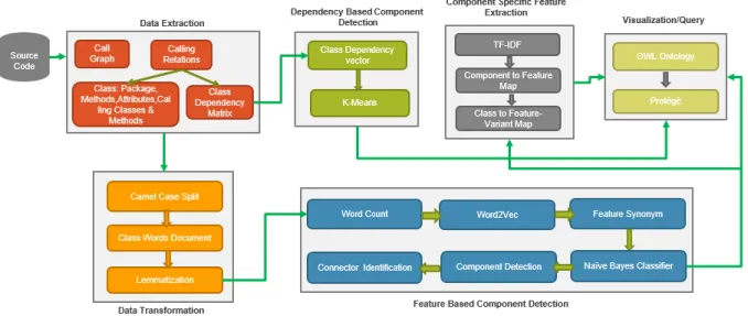
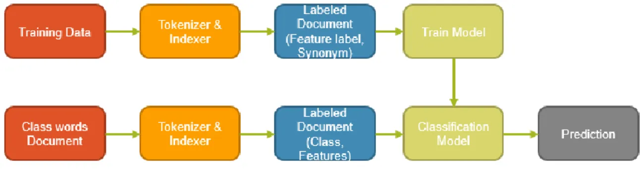
There are two main approaches implemented for component detection and feature extraction of the open source java projects, unsupervised and supervised learning. Two kinds of metadata are extracted for analysis, semantic information and dependency information. Figure 1 shows the overall architecture of the proposed framework. This application is focused on analyzing java projects, so the input to the application is a Java source jar. The architecture of the application consists of six key modules, data extraction, data transformation, feature based component detection, and dependency based component detection, feature extraction, visualization and query processing.
The data extraction component takes care of Metadata generation. The input to the preprocessor is the java source jar. The application generates two different types of Metadata, one based on semantics like package names, class names, method names, attribute names and the other from the calling relationships between the classes. In this step, the metadata is processed to generate class documents and class dependency matrix. All the intermediate documents generated in this approach are stored in the Hadoop distributed file system.
The class documents generated in the data extraction step are then transformed using Natural language processing (NLP) [15] techniques like lemmatization and stemming. The transformed data is then sent to the feature based component detection module. In this module, word count program is used to analyze the important features and Word2Vec [3] machine learning algorithm is used to build the feature synonym vectors which form the training data for the supervised learning algorithms. Machine learning algorithms like Naïve Bayes classifier, Random Forest are used for supervised learning. Once the model is trained using feature synonym vectors, the class metadata documents are
9
used to identify the key feature in each class. The classes are then grouped to form components based on the features identified in supervised learning. The components identified in this module are then passed to the component specific feature extraction module. In this module, TF-IDF [3] is used to identify the key features in each component.
The class dependency matrix created in the data extraction module is used to build the class dependency vectors. These vectors are used as an input to the Means [3] clustering algorithm. K-Means [3] is an unsupervised learning algorithm. It clusters the classes based on the similarities in the dependency relationships. These clusters form the dependency based components for the given project.
The information extracted in the different modules like the features, components, component to class mapping, component to feature mapping, feature to feature variant mapping, class to feature variant mapping etc. are then used to build ontology which can be visualized using Protégé [4] tool and queried using SPARQL [5] query language.
Figure 1: Workflow of Proposed Solution
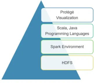
The proposed solution is built on Spark environment. Apache Spark is an open source parallel processing framework. Apache spark provides performance up to 100 times faster compared to Hadoop
10
due to its in-memory storage mechanism. In Spark, data from the software programs can be loaded into the memory of the cluster machines, thus providing faster retrieval of the data. Hence Spark is most suitable for machine learning.
Apache Spark provides Mllib [3] that is a scalable machine learning library. It consists of common machine learning algorithms for classification, regression, clustering, etc. Scala and Java programming languages are used for implementing the program logic. Protégé [4] tool is used for visualization of the ontology generated as part of the thesis.
Figure 2: Implementation Platform
3.2 Data Extraction
Data extraction is the first module of the proposed model. This module is used to extract all the required information from the source code. Since, we have developed this model for Java projects, the input to this module is a source jar. This module consists of four steps: extracting calling relationships using call graph, generating class metadata document, generating class dependency matrix, extracting interfaces.
11
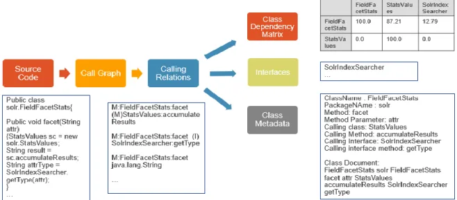
Figure 3: Data Extraction
The following figure shows the complete flow of the data extraction module. In the first step, Java call graph open source project is used to extract the calling relationships from the given source jar. The output of this call graph is then used in the second step to extract the required metadata like the class name, package name, method names, calling classes, calling methods etc. In the third step, the call graph output is used to generate a class dependency matrix by computing the degree of dependency between the classes. Each of the steps implemented in this module are explained in detail in the later sections.
12
3.2.1 Call Graph
Call graph is a directed graph that represents the overall execution of the program and helps in analyzing the calling relationships between different classes. There are two types of call graph: static and dynamic. A static call graph represents every possible run of a program. Whereas a dynamic call graph is more specific and represents only one execution of the program. In this thesis, static call graph information is used for analyzing the features and components in the given project.
Java Call graph [16] is an open source project developed by the Regents of the University of California. We have used this project to extract all the calling relationships available in the source code. Java Callgraph Master [16] is a suite of programs used to generate both static and dynamic call graphs. It can be used both as a library or a command line tool. We have used static call graphs to analyze the calling relationships between various classes in the source code. The call graph program reads byte code of the classes from a jar file, walks down the method bodies and generates a table of caller-caller relationships in the following format:
M:class1:method1 (type of call)class2:method2
This line means that method1 of class1 called method2 of class2. There are four types of calls based on the java opcode: invoke virtual, invoke interface, invoke special, invoke static. The type of call depends on whether the callee is a class or interface or super class etc. For example, if a class calls a method in its super class then it is represented by the opcode invoke special. Similarly, if a class calls a method in an interface, then it is represented by invoke interface. The table 1 below explains the types of calls with examples.
13
Table 1: Call graph Types of Call Type of Call OpCode Instructions Example M for invokevirtual calls Used to invoke instance
methods
M:org.apache.solr.HttpSolrServer:request (M)org.apache.solr.SolrRequest:getMetho d
I for invokeinterface calls Used to invoke methods of interfaces
M:org.apache.solr.HttpSolrServer:request (I)java.util.Collection:iterator
O for invokespecial calls Used to invoke instance initialization methods as well as private methods and methods of a superclass of the current class.
M:org.apache.solr.HttpSolrServer:request (O)org.apache.solr.SolrServerException:<in it>
S for invokestatic calls Used to call the class methods that are declared with the static keyword
M:org.apache.solr.HttpSolrServer:request (S)org.apache.solr.util.ClientUtils:toQueryS tring
Following example explains how the calling relationships are extracted using the opcode in java. The example has 2 classes scheduler, JobImp and an interface Job. The interface Job has only one method: execute. JobImp is a class that implements the interface Job. Scheduler class has two static methods: main, print. The main method in the scheduler class calls the execute method of the interface job and then prints the result using the print static method. The call to the execute method is given the opcode invoke interface and the call to the static method print is given the opcode invoke static in the bytecode. Also, every class in Java is a subclass of the Java.lang.object class, hence it is represented with the opcode invoke special. The below table 2 displays the sample code, the byte code and the output of the call graph.
14
Table 2: Call graph Example
Source Code OpCode for Scheduler Class Callgraph Output for Scheduler class public class Scheduler {Job
job = new JobImpl(); public static void main() { String result = (String) job.execute(); print(result); }
private static void print(String message){
System.out.println(message); }}
public interface Job { Object execute(); }
public class JobImp implements Job { public Object execute(){ Integer value =
createRandomValue(); return incValue(value);
public class Scheduler extends java.lang.Object{
1:invokespecial #1; //Method
java/lang/Object."<init>":()
public void main(); 4: invokeinterface #5, //InterfaceMethod
Job.execute:()Ljava/lang/Object 14: invokestatic #7;
//Method print:(java/lang/String;) private static void
print(java.lang.String); 4: invokevirtual #9; //Method java/io/PrintStream.println:(Ljava/la ng/String;) M:Scheduler:<init> (O)java.lang.Object:<init> M:Scheduler:main (I)Job:execute M:Scheduler:main (S) Scheduler:print$message M:Scheduler:print$message (M)java.io.printStream:print ln
15
3.2.2 Class Document Creation
The output generated from call graph is parsed to extract the required information about the class like the package name, class name, method names, parameters and the calling class names and method names. The metadata extracted about each class is used to create a class metadata document. The class metadata document has the class name followed by all the related words delimited by space.
Format of the class document: ClassName <related words>
Two types of metadata documents are generated for a class: class only, class + dependency. The class only document consists of information about the class like the package name, class name, methods, attributes. The class + dependency also consists of the calling class names and calling method names. While creating the class document, only a substring of package name is included. For example, if the package name is org.apache.solr.search, then only the term search is added to the class document because the portion org.apache.solr is common in all the packages, hence it does not add any value for semantic analysis.
16
3.2.3 Class Dependency Matrix
The call graph output is used to analyze the degree of dependency between the classes. The call graph data presents different types of calling relationships between the classes. The type of dependency determines the closeness between the classes. For example, invoke special is used to call the methods in the super class. Hence it captures the abstraction relation between the classes. Since the classes are closely related to their super classes, the super classes should be given more weightage while computing the degree of dependency. Also, generally a package is a way of grouping related classes. Hence classes within the same package is given more weightage. Similarly, all the calling types are analyzed and a weightage for each type is determined. The following table 3 shows the weightages given to different calling types.
Table 3: Entity Weightage
Resource Weightage Package 20 InvokeSpecial 15 InvokeVirtual 10 InvokeStatic 10 invokeInterface 5
There are three steps for determining the degree of dependency: calculate count, calculate weight, and calculate degree. Firstly, we need to calculate the count that is the number of times a class is being called by the given class. Once the count is determined, we need to identify the type of call and multiply the count with the weightage to obtain the weight. Finally, the degree of dependency on a class is obtained by dividing the class weight with the total weight. The calculations can be represented mathematically as follows.
17
𝑇𝑜𝑡𝑎𝑙 𝑊𝑒𝑖𝑔ℎ𝑡 = ∑ 𝑐𝑜𝑢𝑛𝑡 ∗ 𝑤𝑒𝑖𝑔ℎ𝑡𝑎𝑔𝑒
𝐷𝑒𝑔𝑟𝑒𝑒 = (
𝑐𝑜𝑢𝑛𝑡 ∗ 𝑤𝑒𝑖𝑔ℎ𝑡𝑎𝑔𝑒total weight
* 100)
The following example shows the flows of computation of degree of dependency for a sample
class:
Figure 6: Degree of Dependency Computation
3.2.4 Extracting Interfaces
Call graph identifies the type of calling relationship between the classes. One of the type of calls is invoke interface. This relationship is identified with the letter I. For example, the below output shows that the load method in ManagedResourceStorage is calling the info method in logger interface.
M:org.apache.solr.rest.ManagedResourceStorage:load (I)org.slf4j.Logger:info
From this output, we can extract the interface org.slf4j.Logger. Similarly, all the interfaces present in the source code are extracted. The proposed model could be extended in future to identify the components that implement each of these interfaces extracted and also to classify the interfaces as internal and external interfaces.
18
3.3 Data Transformation
Data transformation is the second module in the proposed model. In this module, the class metadata documents generated in the data extraction module are transformed into a format suitable for analysis. This module has two main steps: camel-Case Split, lemmatization. The output of this module is class words documents. The format of the class words document is given by:
ClassName (\t) relatedWords(delimited by space)
The complete flow of data transformation is explained using an example in the following figure. The details of each of the steps are explained in the following sections.
Figure 7: Data Transformation Example
3.3.1 Camel Case Split
Camel case is a naming convention commonly used in Java. In camel casing two or more words are combined together such that each word begins with a capital letter. So the words need to be split based on this naming convention in order to identify the individual words for semantic analysis. The input to this step is the class metadata document generated in the data extraction module. Each word in the metadata document is split based on camel case naming convention and a class words document
19
is generated. In the class words document, each line holds a class name followed by all the words delimited by space.
Figure 8: Camel Case Split Example
3.3.2 Lemmatization
Lemmatization is a Natural language processing technique. Stanford CoreNLP [15] is used as a library for implementing lemmatization. Stanford CoreNLP is an integrated framework that provides a sets of natural language processing tools for linguistic analysis. Lemmatization basically converts a word to its base form with the use of vocabulary. The base form of a word is known as the lemma. For example: “clients” and “client’s” are converted to “client”. Lemmatization is very crucial for semantic analysis, otherwise the words clients and client are identified as different features. Since the model aims to group the classes to components based on similar features, it is crucial to lemmatize the words to improve accuracy.
In this step, the following transformations are applied to the class words document: 1) Converts a word to its base form
2) Removes stop words
3) Removes special characters like $, &, [] etc. 4) Converts words to lower case.
Stop words are the most common words such as “the”, “is”, “at”, “for” which does not add any value to the semantic analysis for identifying important features. Hence the stop words need to be filtered before processing the data.
20
3.4 Feature Based Component Detection
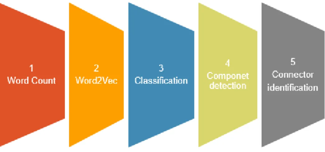
This module finds the components based on the similarity of features in the classes using supervised learning approach. The input to this module is the class words document generated in the data transformation module. The input is processed to identify the important features using word count program, then Word2Vec [3] machine learning algorithm is used to identify the synonyms for these features. Supervised learning algorithms like Naïve Bayes, Random forest are used for classify the classes based on the features. The process in this module can be divided into five steps as shown below:
Figure 9: Feature Based Component Detection Steps
3.4.1 Word Count
Word count program is used to identify the important features. The class words document from the data transformation module is used as an input to this program. The program computes the word count for each class and the words are sorted in the decreasing order of frequency. The top two words for each class are taken and grouped together to identify the key features implemented in the project.
21
Figure 10: Word Count
The below example shows a sample class and the corresponding word count vector. Each class is identified by a unique number. Similarly, each word is identified by a unique number. Two words are picked from each class. The output of this program is a list of important words. The important words for this example are stats, value.
Table 4: Word Count Example
Sample Class Word Count Vector
org.apache.solr.util.stats.Histogram histogram stats sample value clone value clinit clear update sample stats stats clear
update snapshot value
(500,
([0,1,3,7,19,24,47,296,350], [1.0,3.0,2.0,3.0,1.0,1.0,2.0,2.0,1.0]))
3.4.2 Word2Vec
Word2Vec [3] is a neural network language model which takes sequences of words that represents documents and computes distributed vector representation of words. Spark Word2Vec [3] uses skip gram model for representing the words. In skip gram model, each word is associated with 2 vectors say uw and vw which are vector representations of the w as word and context. The main advantage of distributed vector representation is that similar words are closer in the vector space.
22
In our model, we are using Word2Vec [3] to extract the synonyms for the important words identified using the word count program. The synonyms are detected based on the cosine distance between the vectors representing the words. The similarity or the cosine distance between the vectors is computed using the below formula.
The output of the Word2Vec [3] program is a feature synonym vector. For each of the important words, identified in word count program, the synonyms are detected and a feature synonym vector is constructed using the cosine similarity.
Figure 11: Word2Vec [3] Example In this example, the input to the word to vector
program is the “stats” word. Word2Vec [3] analyzes all the words in the class documents and identifies the synonyms for the given word. Synonyms
The synonyms of the word and their cosine distances are used to create the feature synonym
vector as shown in the figure 10.
23
3.4.3 Classification
Supervised Learning algorithms are used for classification of classes based on the features. The following figure demonstrates the steps involved in supervised learning:
Figure 12: Supervised Learning
There are two types of supervised learning algorithms: classification and regression. In our model, we are using the classification algorithms. The classification algorithms classify the given data based on the labeled training data. The feature synonym vectors created using the Word2Vec [3] algorithm form the training data for the classification algorithm. The label is the feature and the synonyms form the data for training. The feature synonym vectors are converted to labeled document and then used for training the model.
The class words documents are then converted to labeled vectors and used for testing the model. The model predicts the key feature in each class document based on the training data. Two classification algorithms are implemented for this purpose: Naïve Bayes classifier and Random Forest. The accuracies of both the algorithms are tested.
Naive Bayesis a multiclass classification algorithm that relies on conditional probability. During training, the Naïve Bayes algorithm computes the conditional probability of the data given the label. Once the model is generated using the training data, Naïve Bayes computes the conditional probability of the label for the given testing data and predicts the label with highest probability.
24
The labeled documents obtained from the feature synonym vectors are used for training the model. Naïve Bayes computes the conditional probability of each synonym given the feature using the following formula:
𝑃(𝑊𝑜𝑟𝑑|𝐿𝑎𝑏𝑒𝑙) =𝑃(Word ᴒ 𝐿𝑎𝑏𝑒𝑙)
𝑃(𝐿𝑎𝑏𝑒𝑙)
The class words documents are used for classifying the classes. During prediction, the algorithm applies Bayes theorem to calculate the conditional probability of the label given the words in the class document and predicts the label with the highest probability.
𝑃(𝐿𝑎𝑏𝑒𝑙|𝑊𝑜𝑟𝑑) = 𝑃(𝑊𝑜𝑟𝑑/𝐿𝑎𝑏𝑒𝑙)𝑃(Word ᴒ 𝐿𝑎𝑏𝑒𝑙)/𝑃(𝑊𝑜𝑟𝑑)
Random Forest [3] is an ensemble of decision trees. The decision tree [3] is a supervised learning classification algorithm that takes a greedy approach to recursively partition the feature space. The tree predicts the same label for all the bottommost leaves. Each partition is chosen by selecting the best split from a set of possible splits to maximize the information gain at a tree node. Random forest [3] creates multiple decision trees in parallel. It incorporates randomness by sampling. For each decision tree, it takes a random subset of training data and a random subset of features. During prediction, random forest aggregates the data from all the decision trees and considers the majority vote.
25
Figure 13: Decision Tree Example
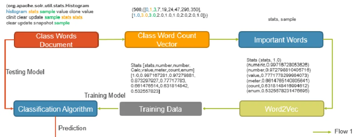
The below example shows the complete flow of feature based component detection module until classification step. The word count program analyzes the important words/features based on the term frequency in the class words document. These features are then passed to Word2Vec [3] to build the feature-synonym vector which is used as training data for the classification algorithm. The model then predicts the feature label for each class using this training data.
Figure 14: Classification Example
3.4.4 Component Detection
Supervised learning algorithm predicts the feature label for each class and outputs a tuple (class, feature). The classes with the same feature are then grouped together to form components. Since the components identified in the module are based on the features implemented in the classes, these components are called as feature based components. The output of this step is a tuple of the format (feature, <List of classes>). The below table gives an example of the components detected using this approach.
26
Table 5: Feature Based Component Example
Input tuple(class, feature) Output tuple ( feature , <List of classes>) (org.apache.solr.ParseIntFieldUpdateProcessorFact ory,processor) (org.apache.solr.ConcatFieldUpdateProcessorFacto ry,processor) (org.apache.solr.StatelessUpdateProcessorFactory, processor) (org.apache.solr.StandardRequestHandler, handler) (org.apache.solr.BinaryUpdateRequestHandler, handler) (processor, org.apache.solr.ParseIntFieldUpdateProcessorFactory, org.apache.solr.ConcatFieldUpdateProcessorFactory, org.apache.solr.StatelessUpdateProcessorFactory) (handler, org.apache.solr.StandardRequestHandler, org.apache.solr.BinaryUpdateRequestHandler)
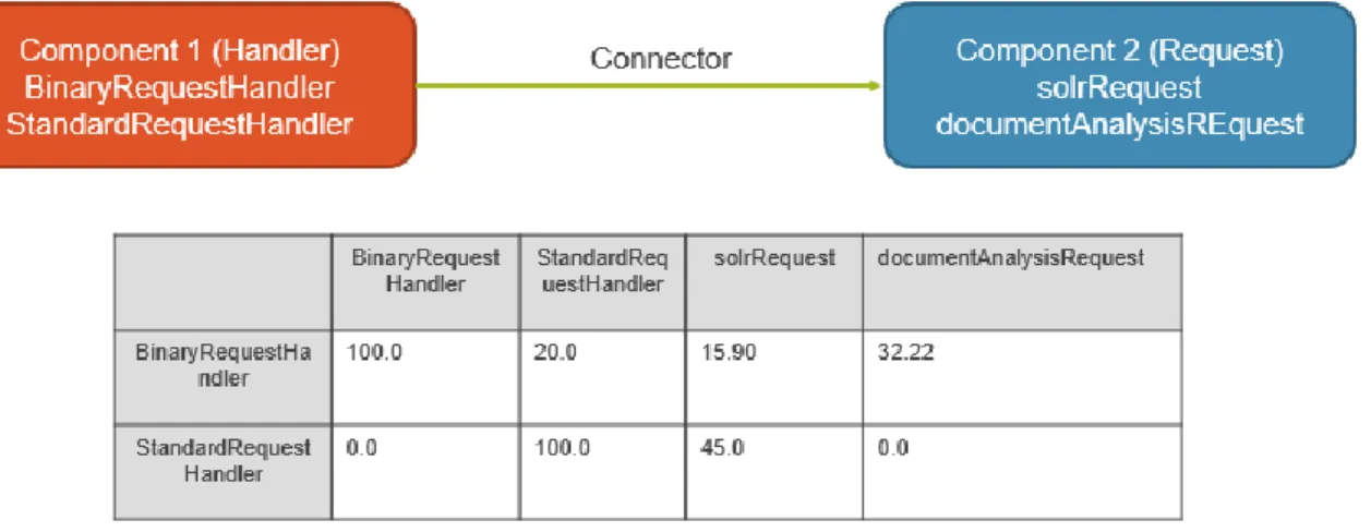
3.4.5 Connector Identification
Connector is a directed dependency relation between components. If any class A in component-1 is dependent on any class B in component-2, then a directed relationship is established between these components from component-1 to component-2. The degree of dependency is identified using the class dependency matrix generated in the data extraction step. This degree of dependency is then used to analyze the dependencies between the classes in different components. The connector could be unidirectional or bidirectional depending on the calling relationships among the classes in different components.
27
Figure 15: Connector Example
3.5 Dependency Based Component Detection
Dependency based component detection uses an unsupervised learning approach for identifying the components based on the calling relationships between the classes. The class dependency matrix generated in the data extraction module is used for building the class dependency vector. The class dependency vector gives the degree of dependency of a class on all the classes in the project. If a class A is not dependent on another class B, then the degree of dependency will be zero. The degree of dependency on itself will be given as 100.0.
Sample class dependency vector:
org.apache.solr.store.hdfs.HdfsDirectory,0.0,0.0,33.333333333333335,67.333333333333335,100.0 Once the vectors are generated, K-Means [3] clustering algorithm is used to cluster the classes into components. K-Means is an unsupervised learning algorithm used for clustering the data. K-Means algorithm classifies the data into a given number of clusters (k) by defining the centroids for each cluster. To ensure best clustering these centroids should be placed as far away as possible from each other. Once the centroids are determined, each point in the feature space is assigned to its nearest centroid. Once
28
the clusters are identified, we to recalculate the centroid for each cluster. Then the data points are remapped to their nearest centroids. This process is iterated until there is no change in the centroids.
The number of clusters K in the K-Means clustering is unknown. To determine the k value, the K-Means algorithm is executed for different cluster sizes and the sum of squared error (SSE) is computed. The K-value that gives the least sum of squared distance or the k-value at which there is not much difference in the SSE is chosen as the final cluster size.
The output of the K-Means will be tuple (class, component-number). The classes with the same component prediction are grouped together and a new tuple is generated in the format (component-number, <List of classes>).
3.6 Component Specific Feature Extraction
Each component consists of many classes that implement a number of features. This step is used to identify the key features implemented by each of the components. The input for this step could be the components detected from supervised or unsupervised learning approaches. Features in the components are detected by using semantic analysis. The high level flow of feature extraction from the components is shown in figure 15. It has four steps. In the first step, the data from the class documents of all the classes within a component are aggregated to form the component words document.
29
Figure 16: Component Specific Feature Extraction
The component words documents are then passed to the Term Frequency-Inverse Document Frequency (TF-IDF) for feature extraction. TF-IDF [3] is the product of term frequency and inverse document frequency. The term frequency is the number of times a word appears in a specific document. Document frequency is the frequency of the term in all the documents. The Inverse document frequency intends to reduce the importance of the word that occurs most frequently in all the documents. It is mainly used to eliminate the common terms across all the documents. The IDF value is computed by diving the total number of documents with the number of documents that contain the given term t and then applying logarithm to the resultant value. If the term appears in more documents, it is more likely to be a common term that is not specific to any given document, hence the log value of the word reduces to zero ensuring that the IDF value and thereby the TF-IDF value is less for this term.
: the total number of documents
: the number of documents in which the term appears The TF-IDF is calculated using the following formula:
30
TF-IDF value is high if the term has high term frequency and a low document frequency in the whole collection of documents. Hence by considering the TF-IDF value, we can eliminate the common terms in determining features.
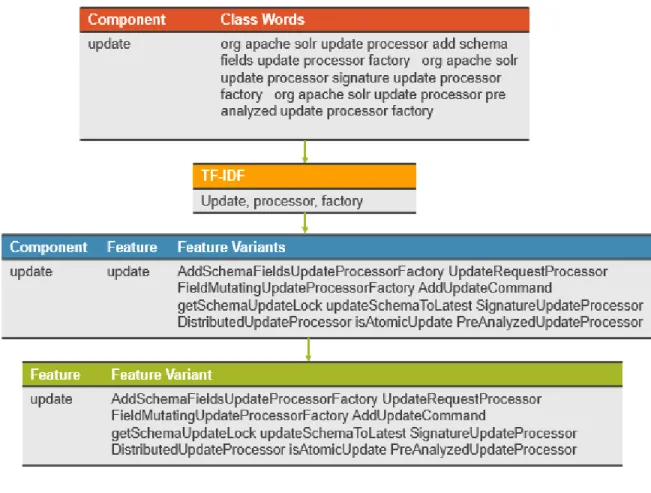
For each component, the words are sorted based on the TF-IDF [3] values and top three features are extracted. The output of this step is a tuple of the format (Component, <List of Features>). Since the features are individual words obtained after splitting the class/method names based on camel casing, the words are traced back to obtain the full words from the class metadata documents. The full words are called as the feature variants. Once the feature variants are extracted, tuples of the format (feature, <List of feature variants>) are created. These tuples are then mapped to the component. Also while identifying the feature variants, the class from which the variant is obtained is determined to create a class to feature variant mapping.
It is possible that a feature is implemented in different components. The feature variants implemented by different components could be different. Hence we need to aggregate the (feature, <List of feature variants>) tuples generated from all the components to obtain the final feature to feature variant mapping. Following example shows the mapping created at each step of this module.
31
Figure 17: Feature Extraction Example
3.7 Ontology and Query Processing
Ontology is the description of concepts and the relationships that exists between them. It deals with identifying the entities, their relationships and representing them in a hierarchy such that similar entities are grouped together. Software Ontology [17] is a way of describing the software in terms of information like platform, version, types and properties of software components, features and relationships between them.
OWL [18] is a standard web ontology language proposed by W3C. It is an extension of RDF (the Resource Description Framework). RDF is an assertion model to represent the resources available on the web in the form of RDF triples of ”subject”, ”predicate” and ”object”. However, RDF schema doesn’t provide means to represent the relationships between classes and properties. OWL is used to represent
32
classes and their interrelationships. An OWL Class defines a group of individuals that share common properties. For example “Person” is a class. OWL Individual is an instance of the class. For example “John” is an individual of the class “Person”.
OWL provides a richer set of vocabulary for defining properties and imposing restrictions on them. There are two types of properties in OWL, Datatype properties and object properties. Object properties represent relationships among individuals and datatype properties are used to assign data values to individuals. For Example: “hasParent” is an Object property while “hasAge” is a data property. In OWL, we can define properties as reflexive, transitive, symmetric, functional, and inverse. OWL class properties like equivalent class, subclass of, disjoint class can be used to represent the relationships between classes. Thus various relationships and restrictions can be imposed on the classes in OWL. OWL is mainly used to provide meaningful descriptions to the terminology and the information on the web to enable reasoning on the web documents.
OWL API [23] is an open source java API for importing, creating and manipulating OWL ontologies. It is primarily maintained by University of Manchester. The latest version of OWL API is based on OWL 2 specification which includes OWL-Lite, OWL-DL and some elements of OWL-Full. They are all sub languages of OWL with some variations and differences in restrictions. OWL-Lite is more restrictive compared to OWL-DL and OWL-Full. It allows representation of hierarchies with some constraints. OWL-Full is syntactically similar to RDF and it doesn’t have any restrictions like OWL-Lite.
This thesis aims at generating a model that represents the software project which can be queried to search for functionality. We have used OWL 2.0 Ontology to represent the project. The ontology of a project is built using the information generated in the previous modules. Software ontology [22] is used as a base for generating the project ontology. Software ontology is developed at Information Sciences Institute in University of South California. It is a resource for describing the aspects of a software architecture like software types, operating system of the software, programming
33
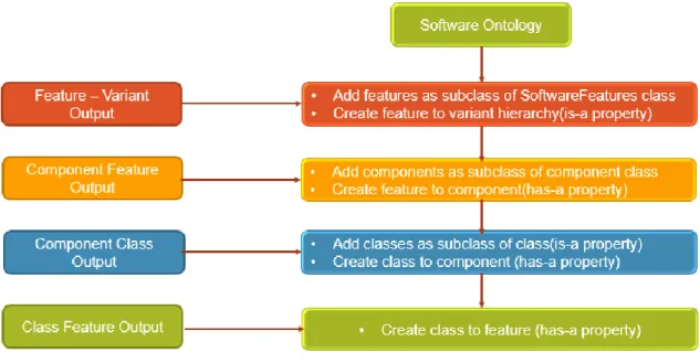
languages, software components, packages, domains, etc. This ontology is most suitable for our requirement as it provides a means to describe most of the concepts and their relationships in software architecture. We have extended this ontology as per our requirements. The following figure 17 represents the software ontology as visualized in protégé using OWL Viz.
Figure 18: Software Ontology
FeatureDomain class is added as a subclass to software domains class. All the features discovered in the feature extraction process are added as subclasses to the feature domain class. Each feature has a set of feature variants. The feature variants are connected to their respective features using subclass relationship.
Software ontology has a software component class. All the components detected using supervised learning approach are added as subclasses to this class. Each component has a set of classes. All the classes within a component are connected to the component using a subclass object property.
The component to feature mapping obtained in the component specific feature extraction module is used to establish the relationship between the components and features. An object property “hasComponent” is created. And all the components implementing a specific feature are connected to this feature using this property. Similarly all feature variants are connected to their respective classes using the class to feature variant mapping. Figure 18 displays the steps involved in generating the ontology for a given model using the different outputs generated in the previous modules.
34
Figure 19: Ontology Generation
The generated ontology is visualized using Protégé [4] tool. Protégé is an open source ontology editor developed at Stanford University in collaboration with University of Manchester. It provides an interface to define ontologies, query ontologies and visualize them. OWL Viz [19] is used to represent the class hierarchy in Protégé. OWL Viz is a plugin that depends on Graphviz [21] that is a visualization software that represents structural information as diagrams of abstract graphs and networks. Ontograf [20] is a plugin used for visualizing the object properties and the relationships between various classes in the ontology. It provides a search functionality using which we can search for any feature and it displays all the features with that name and the components/classes implementing that feature.
One of the key advantages of building an ontology to represent the software is that the ontology can be queried using any RDF querying language like SPARQL [5]. SPARQL is a semantic query language used for retrieving and manipulating data stored in RDF format. SinceOWL is an extension of RDF. SPARQL can be used to query OWL Ontology. There are two ways for querying OWL Ontologies:
1) Using Jena API and writing a java program with embedded SPARQL query/create an interface to provide the SPARQL query
35 2) Using SPARQL plugin in Protégé
In this thesis, we have used the SPARQL plugin in Protégé to query the generated ontology and do some reasoning on the same. Following are some of the use cases for query analysis:
1) Get the list of Features
2) Identify components implementing a feature
3) Get the list of variants for a feature
4) Identify the classes implementing a feature variant 5) Get the connections/dependencies between components
36 CHAPTER 4
RESULTS AND EVALUATION
This thesis builds a model of a software project from the source code dynamically. For building the model, it analyze the features, components and connectors. Two types of components are detected using the proposed solution. Feature based components are groups of classes implementing similar features. Dependency based components are groups of classes that have higher degree of dependency. Component definition changes based on perspective. So depending on the developers use case, one could use the respective component structure for their analysis. The proposed model also identifies the connectors which are directed relationships between the components. Two projects are analyzed as part of case studies: Apache Solr and Apache Lucene. The following sections present the results from both the projects and the interaction between the components in these projects.
4.1 Apache Solr
Apache Solr is an open source search platform built using Apache Lucene and written in Java. Apache Solris used as a case study for the approach proposed in the thesis. Apache Solr is a highly reliable and scalable open source search server. Below are the statistics of the Apache Solr project generated using Java call graph. Solr has 836 classes and lots of features and dependencies which makes it a good candidate for feature based and dependency based analysis using our proposed model. The key assumption for the feature based analysis is that the names used for code entities reflect their functionality and follow camel case.
37
Table 6: Apache Solr Statistics
Entity Number Dependencies 84692 Packages 176 Classes 836 Methods 8396 Parameters 1812
Apache Solr has 836 classes with many methods and dependencies. Java call graph project is used for identifying all the static dependencies in the given software project. Below is the sample output from the call graph.
Table 7: Sample Call graph output
ClassName:MethodName$parameter (typeOfCall)ClassName:MethodName$parameter M:org.apache.solr.handler.component.FieldFac etStats:getStatsValues (I)java.util.Map:get M:org.apache.solr.handler.component.FieldFac etStats:getStatsValues (S)org.apache.solr.handler.component.StatsValuesFa ctory:createStatsValues M:org.apache.solr.handler.component.FieldFac etStats:getStatsValues (I)org.apache.solr.handler.component.StatsValues:se tNextReader M:org.apache.solr.handler.component.FieldFac etStats:facet (M)org.apache.lucene.queries.function.FunctionValu es:exists M:org.apache.solr.handler.component.FieldFac etStats:facet (M)org.apache.lucene.queries.function.FunctionValu es:strVal M:org.apache.solr.handler.component.FieldFac etStats:facet (O)org.apache.solr.handler.component.FieldFacetSta ts:getStatsValues M:org.apache.solr.handler.component.FieldFac etStats:facet (I)org.apache.solr.handler.component.StatsValues:ac cumulate
38
Below table shows the call graph statistics for a sample set of classes in Apache Solr. It displays the number of methods, attributes, calling classes, calling methods, etc for a class.
Table 8: Sample Callgraph Statistics
Class Methods Attributes
Calling Classes Calling Methods org.apache.solr.core.SolrCore 95 15 85 96 org.apache.solr.search.SolrIndexSearcher 94 16 43 59 org.apache.solr.schema.IndexSchema 80 12 20 40 org.apache.solr.cloud.ZkController 71 12 40 104 org.apache.solr.search.ExtendedDismaxQParser 68 14 17 40 org.apache.solr.schema.FieldType 65 3 14 36 org.apache.solr.cloud.OverseerCollectionProcessor 63 14 43 131 org.apache.solr.cloud.Overseer 58 15 25 67 org.apache.solr.update.UpdateLog 55 14 26 56 org.apache.solr.handler.component.ResponseBuilder 54 2 12 23 org.apache.solr.handler.SnapPuller 53 21 31 50 org.apache.solr.core.CoreContainer 47 3 24 79 org.apache.solr.core.ConfigSolr 47 3 12 13 org.apache.solr.update.TransactionLog 46 8 11 21 org.apache.solr.util.ConcurrentLRUCache 46 8 0 0
39
4.1.1
Feature Based Analysis
The proposed model discovers two types of components: feature based components, dependency based components. Feature based components are groups of classes that implement similar features. Features in the given project are detected using semantic analysis. For semantic analysis, two sets of input data are generated. The class only documents consist of all the words related to the class like the package name, class name, method names, and attribute names. Class+Dependency data consist of all words related to class like package name, class name, method names, attribute names, calling class names, calling method names. The following figure shows the difference in the content of the class only and Class+Dependency input data.
Figure 20: Class Only vs Class + Dependency Input Data
Both the class documents are analyzed to identify the features and components using the same set of steps. Firstly, each of these words in the class documents are split using camel case naming convention and then lemmatized to convert the words to their base form. Without lemmatization the words “values” and “value” are treated as different features. Since the approach uses semantic analysis, it is required to convert all the words to their base forms for more accuracy. Also, stop words like “the”, “get”, “set” are removed during lemmatization of the class documents. Hence for identifying the important features, we could use word count. Word count is basically the frequency of terms in the
40
class document. From each class document, the top two words are taken based on the decreasing order of frequency. The following figure shows the set of important words/features identified for Apache Solr project using the Class+Dependency documents.
Figure 21: Apache Solr Important Words
During development, different words may be used to represent the same functionality. For example output and result represent the same function. Hence it is required to identify the synonyms of the important words identified using word count program so that classes that contain the important word or their synonyms can be grouped together for identifying the feature based components. As mentioned before, Word2Vec [3] is a machine learning algorithm that represents words in the form of distributed vectors and identifies the similarity between the words using cosine distance. Thus synonyms can be detected based on the cosine similarity between the words. The important words and their synonyms are used to create the feature synonym data. This data is used for training the supervised learning algorithms. The class documents are then used for testing the algorithm which classifies the classes. The classification of the classes is tested using two supervised learning algorithms: Naïve Bayes and Random Forest. It is observed that the accuracy of Naïve Bayes (87.16%) is more
41
compared to the Random Forest (68.75%) algorithm for semantic analysis. Below tables show the classification output using Naïve Bayes algorithm for class only and Class+Dependency documents.
Table 9: Naïve Bayes Classification Output for Class only Data
Class Feature org.apache.solr.rest.SolrSchemaRestApi schema org.apache.solr.util.plugin.NamedListPluginLoader plugin org.apache.solr.cloud.LeaderInitiatedRecoveryThread leader org.apache.solr.search.Grouping facet org.apache.solr.spelling.AbstractLuceneSpellChecker diagnostic org.apache.solr.handler.component.DateStatsValues stats org.apache.solr.update.processor.RemoveBlankFieldUpdateProcessorFactory processor org.apache.solr.util.RTimer diagnostic org.apache.solr.update.processor.StatelessScriptUpdateProcessorFactory processor org.apache.solr.common.cloud.HashBasedRouter hash org.apache.solr.update.processor.CloneFieldUpdateProcessorFactory processor org.apache.solr.common.cloud.RoutingRule route org.apache.solr.search.SpatialFilterQParserPlugin filter org.apache.solr.schema.BBoxField field
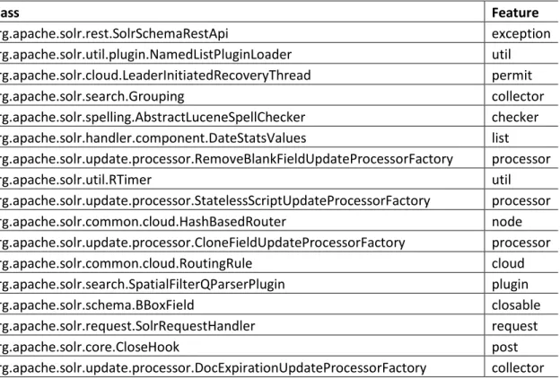
Table 10: Naïve Bayes Classification output for Class + Dependency Data
Class Feature org.apache.solr.rest.SolrSchemaRestApi exception org.apache.solr.util.plugin.NamedListPluginLoader util org.apache.solr.cloud.LeaderInitiatedRecoveryThread permit org.apache.solr.search.Grouping collector org.apache.solr.spelling.AbstractLuceneSpellChecker checker org.apache.solr.handler.component.DateStatsValues list org.apache.solr.update.processor.RemoveBlankFieldUpdateProcessorFactory processor org.apache.solr.util.RTimer util org.apache.solr.update.processor.StatelessScriptUpdateProcessorFactory processor org.apache.solr.common.cloud.HashBasedRouter node org.apache.solr.update.processor.CloneFieldUpdateProcessorFactory processor org.apache.solr.common.cloud.RoutingRule cloud org.apache.solr.search.SpatialFilterQParserPlugin plugin org.apache.solr.schema.BBoxField closable org.apache.solr.request.SolrRequestHandler request org.apache.solr.core.CloseHook post org.apache.solr.update.processor.DocExpirationUpdateProcessorFactory collector