The Effect of Noise and Sample Size on an Unsupervised Feature
Selection Method for Manifold Learning
Alfredo Vellido and Jorge Velazco
Abstract— The research on unsupervised feature selection is
scarce in comparison to that for supervised models, despite the fact that this is an important issue for many cluster-ing problems. An unsupervised feature selection method for general Finite Mixture Models was recently proposed and subsequently extended to Generative Topographic Mapping (GTM), a manifold learning constrained mixture model that provides data visualization. Some of the results of a previous partial assessment of this unsupervised feature selection method for GTM suggested that its performance may be affected by insufficient sample size and by noisy data. In this brief study, we test in some detail such limitations of the method.
I. INTRODUCTION
T
HE fields of machine learning and statistics coexist with data analysis as a common target and they overlap in what has come to be defined as Statistical Machine Learning. An example of this can be found in Finite Mixture Mod-els, which are flexible and robust methods for multivariate data clustering [1]. The addition of visualization capabilities would benefit these models in many application scenarios, helping to provide intuitive cues about data structural pat-terns. One way to endow Finite Mixture Models with data visualization is by constraining the mixture components to be centered in a low-dimensional manifold embedded into the multivariate data space, as in Generative Topographic Mapping (GTM) [2]. This is a manifold learning model for simultaneous data clustering and visualization.The interpretability of the clustering results provided by GTM becomes difficult when the analyzed data sets con-sist of a large number of features. This limitation can be overcome with methods to estimate the ranking of the data features according to their relative relevance, leading to feature selection (FS). The research on unsupervised FS is scarce in comparison to that for supervised models, despite the fact that FS becomes an issue of paramount importance for many clustering problems, regardless the unavailability of class labels. The interpretability of the clusters obtained by unsupervised methods would be improved by their de-scription in terms of a reduced subset of relevant variables. An important advance on unsupervised FS for Finite Mixture Models was presented in [3] and recently extended to GTM in [4] and to one of its variants for time series analysis in [5]. This method was preliminarily assessed in [6], where some of the results suggested that the performance of the method may be degraded by characteristics of the data such as insufficient sample size and the presence of noise.
Department of Computing Languages and Systems (LSI). Technical University of Catalonia (UPC). C. Jordi Girona, 1-3. 08034, Barcelona, Spain (email:{avellido, e00728496}@lsi.upc.edu).
Alfredo Vellido is a researcher within the Ram ´on y Cajal program of the Spanish Ministry of Education and Science (MEC) and acknowledges funding from the MEC I+D project TIN2006-08114
In this brief study, we provide far more detailed evidence of the limitations of the method through controlled experiments using synthetic data.
The remaining of the paper is organized as follows. First, brief introductions to the standard Gaussian GTM and its extension for Feature Relevance Determination (FRD) are provided in section 2. This is followed, in section 3, by a description of the experimental settings and, in section 4, by a presentation and discussion of the results. The paper closes with a brief summary of conclusions.
II. FEATURERELEVANCEDETERMINATION FORGTM
A. The Standard GTM Model
The neural network-inspired GTM is a manifold learn-ing model with sound foundations in probability theory. It performs simultaneous clustering and visualization of the observed data through a nonlinear and topology-preserving mapping from a visualization latent space in L (with L
being usually 1 or 2 for visualization purposes) onto a manifold embedded in the D space, where the observed data reside.
For each feature d, the functional form of this mapping is the generalized linear regression model yd(u,W) =
M
mφm(u)wmd, where φm is one of M basis functions,
defined here as spherically symmetric Gaussians, generating the non-linear mapping from a latent vectoruto the manifold in D. The matrixWof adaptive weightsw
md explicitely
defines this mapping.
The prior distribution ofuin latent space is constrained to form a uniform discrete grid ofKcentres. A density model in data space is therefore generated for each componentkof the mixture, which, assuming that the observed data setXis constituted byN independent, identically distributed (i.i.d.) data points xn, leads to the definition of a complete
log-likelihood in the form:
L(W,β|X)= N n=1ln 1 K K k=1(2πβ)D/2exp{−β/2yk−xn2} (1)
whereykis a reference or prototype vector consisting of
ele-ments (ydk=
M
m φm(uk)wmd), which are an instantiation
of the generalized linear regression model described above. From Eq. (1), the adaptive parameters of the model, which are W and the common inverse variance of the Gaussian components, β, can be optimized by maximum likelihood (ML) using the Expectation-Maximization (EM) algorithm. Details can be found in [2].
B. The FRD-GTM
The problems of feature selection and feature relevance determination are commonly understood as one of the pos-sible strategies for data dimensionality reduction, usually
523 978-1-4244-1821-3/08/$25.00 c2008 IEEE
for supervised problems. In such setting, a data feature is said to be relevant (and it is eventually selected) only if its absence (or its absence in combination with the absence of others) worsens significantly the classification or predictive performance of the defined model. Feature selection and feature relevance determination for unsupervised learning, even if sharing the dimensionality reduction objective of their supervised counterparts, are far less investigated problems. Here, the relevance is not longer related to a label or target variable, and various feature ranking criteria can be considered, including, but not limited to, saliency, entropy,
smoothness, densityand reliability [7].
In this paper, unsupervised feature relevance is understood as the likelihood of a feature being responsible for generating the data cluster structure. Therefore, relevant features will be those which better separate the natural clusters in which the data are structured. Moreover, we are interested in unsupervised feature selection methods that are suitable for clustering models that also provide data visualization. With that in mind, the FRD technique was defined for the GTM model in [4]. For the unsupervised GTM clustering model, relevance is defined through the concept of saliency.
The FRD problem was investigated for GTM in [4]. Feature relevance in this unsupervised setting is understood as the likelihood of a feature being responsible for generating the data cluster structure. In this unsupervised setting, rele-vance is defined through the concept of saliency. Formally, the saliency of featuredcan be defined asρd=P(ηd= 1),
whereη=(η1, . . . , ηD)is a set of binary indicators that can
be integrated in the EM algorithm as missing variables. A value of ηd = 1 (ρd= 1) indicates that feature dhas the
maximum possible relevance. According to this definition, the FRD-GTM mixture density can be written as:
p(x|W,β,w0,β0,ρ)= K k=1K1 D d=1{ρdp(xd|uk;wd,β)+(1−ρd)q(xd|u0;w0,d,β0,d)} (2) where wd is the vector of W corresponding to feature d
and ρ ≡ {ρ1, . . . , ρD}. A feature d will be considered irrelevant, with irrelevance (1−ρd), if p(xd|uk;wd, β) =
q(xd|u0;w0,d, β0,d)for all the mixture componentsk, where qis a common density followed by feature d. Notice that this is like saying that the distribution for feature d does not follow the cluster structure defined by the model. This common component requires the definition of two extra adaptive parameters in (2): w0 ≡ {w0,1, . . . , w0,D} and
β0≡ {β0,1, . . . , β0,D}(so thaty0=φ0(u0)w0). For fully relevant (ρd→1) features, the common component variance
vanishes:(β0,d)−1 → 0. The parameters of the model can,
once again, be optimized by ML using the EM algorithm. Detailed calculations can be found in [8].
III. EXPERIMENTALSETTINGS
The results of statistically principled models for proba-bility density estimation, such as GTM and its variants, are bound to be affected, in one way or another, by sample size and by the presence of uninformative noise in the data. Here, we assess such effects on the FRD-GTM model described in the previous section. For that, data with very specific characteristics are required. We use synthetic sets similar to those in [3] for comparative purposes.
The first synthetic set (hereafter referred to assynth1) is a variation on theTrunkdata set used in [3]), and was designed for its 10 features to be in decreasing order of relevance. It consists of data sampled from two Gaussians N(μ1,I)
and N(μ2,I), where:
μ1= 1,√13, . . . ,√21d−1, . . . ,√119
and μ1 = −μ2. We hypothesize (H1) that the feature
relevance ranking estimated by FRD-GTM for these data will deteriorate gradually as sample size decreases. Samples
ofsynth1of different sizes, from 100 to 10,000 points, were
used in this study to testH1. It is also hypothesized (H2) that the feature relevance ranking will deteriorate in proportion to the level of noise. In order to testH2, four increasing levels of Gaussian noise, of standard deviations 0.1, 0.2, 0.5, and 1, were added to the 10 original features ofsynth1, for a given sample size.
The second dataset (hereafter referred to assynth2) con-sists of a contrasting combination of features: the first two define four neatly separated Gaussian clusters with centres located at(0,3),(1,9),(6,4)and(7,10); they are meant to be relatively relevant. The next four features are Gaussian noise and, therefore, rather irrelevant in terms of defining cluster structure. Similar experiments to the ones devised for
synth1were designed to further testH1andH2.
The FRD-GTM parameters W and w0 were initialized with small random values sampled from a normal distri-bution. Saliencies were initialized at ρd = 0.5,∀d, d =
1, . . . , D. The grid of GTM latent centres was fixed to a square layout of 3×3 nodes (i.e., 9 constrained mixture components). The corresponding grid of basis functionsφm
was fixed to a2×2layout.
IV. EXPERIMENTAL RESULTS AND DISCUSSION
The experiments outlined in the previous section aim to assess the effect of sample size and the presence of noise on the performance of FRD-GTM in the process of unsupervised feature relevance estimation.
A. The Effect of Sample Size
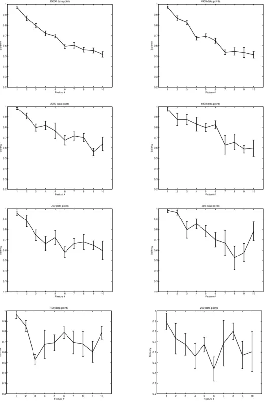
The FRD ranking results forsynth1are shown in Fig. 1, for sample sizes from 10,000 down to 100 points. Further sample sizes were tested, conforming to a similar pattern; their results are not included for the sake of brevity. A deterioration of the results is clearly observed for datasets of less than 1,000 points. This deterioration takes two forms: Firstly, a breach of the expected monotonic decrease of the mean feature saliencies. Secondly, a neat increase of uncertainty in the results, illustrated in Fig. 1 in the form of bigger bars of the standard deviation of the estimated saliencies. As a result, the confidence on the validity of the results for small sample sizes decreases considerably. According to these results,H1is at least partially supported. The FRD ranking results forsynth2, again for sample sizes from 10.000 down to 100 points, are shown in Fig. 2. This is an easier problem for the model, and this is reflected by the fact that the saliency estimated for the two first features is higher than that estimated for the rest of the features, even for a sample size as small as 100 points.
1 2 3 4 5 6 7 8 9 10 0.2 0.3 0.4 0.5 0.6 0.7 0.8 0.9 1 Feature # Saliency 10000 data points 1 2 3 4 5 6 7 8 9 10 0.2 0.3 0.4 0.5 0.6 0.7 0.8 0.9 1 Feature # Saliency 4000 data points 1 2 3 4 5 6 7 8 9 10 0.2 0.3 0.4 0.5 0.6 0.7 0.8 0.9 1 Feature # Saliency 2000 data points 1 2 3 4 5 6 7 8 9 10 0.2 0.3 0.4 0.5 0.6 0.7 0.8 0.9 1 Feature # Saliency 1000 data points 1 2 3 4 5 6 7 8 9 10 0.2 0.3 0.4 0.5 0.6 0.7 0.8 0.9 1 Feature # Saliency 750 data points 1 2 3 4 5 6 7 8 9 10 0.2 0.3 0.4 0.5 0.6 0.7 0.8 0.9 1 Feature # Saliency 500 data points 1 2 3 4 5 6 7 8 9 10 0.2 0.3 0.4 0.5 0.6 0.7 0.8 0.9 1 Feature # Saliency 400 data points 1 2 3 4 5 6 7 8 9 10 0.2 0.3 0.4 0.5 0.6 0.7 0.8 0.9 1 Feature # Saliency 200 data points
Fig. 1. Experiments with differentsynth1sample sizes (indicated in the plot titles) Mean salienciesρdfor the 10 features. The bars span from the mean minus to the mean plus one standard deviation of the saliencies over 20 runs of the algorithm.
1 2 3 4 5 6 0 0.1 0.2 0.3 0.4 0.5 0.6 0.7 0.8 0.9 1 Feature # Saliency 10000 data points 1 2 3 4 5 6 0 0.1 0.2 0.3 0.4 0.5 0.6 0.7 0.8 0.9 1 Feature # Saliency 4000 data points 1 2 3 4 5 6 0 0.1 0.2 0.3 0.4 0.5 0.6 0.7 0.8 0.9 1 Feature # Saliency 2000 data points 1 2 3 4 5 6 0 0.1 0.2 0.3 0.4 0.5 0.6 0.7 0.8 0.9 1 Feature # Saliency 1000 data points 1 2 3 4 5 6 0 0.1 0.2 0.3 0.4 0.5 0.6 0.7 0.8 0.9 1 Feature # Saliency 400 data points 1 2 3 4 5 6 0 0.1 0.2 0.3 0.4 0.5 0.6 0.7 0.8 0.9 1 Feature # Saliency 300 data points 1 2 3 4 5 6 0 0.1 0.2 0.3 0.4 0.5 0.6 0.7 0.8 0.9 1 Feature # Saliency 200 data points 1 2 3 4 5 6 0 0.1 0.2 0.3 0.4 0.5 0.6 0.7 0.8 0.9 1 Feature # Saliency 100 data points
A deterioration of the saliency estimation is nevertheless evident for the smallest of the sample sizes investigated. This is consistent with the results for synth1 and, again, H1 is partially supported.
B. The effect of Noise
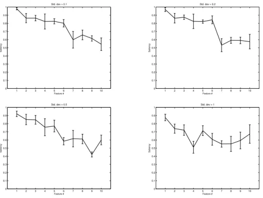
In the experiments reported in Fig. 3, four levels of Gaussian noise of increasing level were added to a sample of 1,000 points ofsynth1. The FRD-GTM is shown to behave robustly even in the presence of a substantial amount of noise, although its performance deteriorates significantly for noise of standard deviation = 1, as reflected in the breach of the expected monotonic decrease of the mean feature saliencies. H2 is, therefore, partially supported by these results.
Fig. 4 displays the results of a similar experiment for
synth2. They are fully consistent with those obtained with
synth1. The model again behaves robustly in the presence of
noise and clearly deteriorates at the highest level of added noise, for which the model struggles to distinguish the first two features from the purely noisy ones. HypothesisH2 is, again, at least partially supported.
This support for hypothesisH2is, even if partial, certainly not unexpected. As robust as it may be, the FRD-GTM model is still prone to data overfitting. That is, at some point, the model will start learning the noise as much as learning the underlying signal distributions. The resulting FRD-GTM model will be over-complex and, if the noise is uninformative (i.e., in this case, if the noise affects all data features equally), the method of relevance determination will eventually start struggling to provide correct saliency estimations. One way around this problem is to endow the model with regularization capabilities to effectively control complexity [9], [10], [11]. FRD-GTM is thus likely to benefit from the definition of extensions of the model encompassing adaptive regularization.
V. CONCLUSIONS
In this paper, the effects of sample size and the presence of noise on a method of unsupervised feature relevance determination for the manifold learning GTM model, have been investigated in some detail. The FRD-GTM has been shown to behave with reasonable robustness even at small sample sizes and in the presence of a fair amount of noise. Even though, performance deterioration has been observed at very small sample sizes and in the presence of high level of noise.
This relative weakness of the method in the presence of noise makes it convenient to consider possible strategies for model regularization and, therefore, future research will be devoted the design of methods for automatic and proactive model regularization to prevent or at least limit the negative effect of data overfitting on the FRD method for GTM. Some of such methods have already been designed for the standard GTM formulation [9], [10] and could be extended to FRD-GTM. Alternatively, regularization could be accomplished through a reformulation of the GTM within a variational Bayesian theoretical framework [11]. Again, this could be extended to accomodate FRD.
Future research should also extend the current experimen-tal design to include a wider variety of artificial data sets of different characteristics, as well as to include comparisons with alternative unsupervised feature relevance determitation and feature selection techniques.
REFERENCES
[1] G. J. McLachlan and D. G. Peel.Finite mixture models. New York:
John Wiley-Sons, 2000.
[2] C. M. Bishop, M. Svens´en and C. K. I. Williams. “GTM: The
Genera-tive Topographic Mapping”.Neural Computation, 10(1), pp. 215–234,
1998.
[3] M. H. C. Law, M.A.T. “Figueiredo and A. K. Jain, Simultaneous Feature Selection and Clustering Using Mixture Models”,IEEE T. Pattern Anal, 26(9), pp. 1154–1166, 2004.
[4] A. Vellido, P. J. G. Lisboa and D. Vicente, “Robust Analysis of MRS
Brain Tumour Data Using t-GTM”,Neurocomputing, 69(7–9), pp. 754–
768, 2006.
[5] I. Olier and A. Vellido, “Time Series Relevance Determination through a topology-constrained Hidden Markov Model”,In Proc. of the 7th In-ternational Conference on Intelligent Data Engineering and Automated Learning (IDEAL 2006), Burgos, Spain. LNCS 4224, pp. 40–47, 2006. [6] A. Vellido, “Assessment of an Unsupervised Feature Selection Method
for Generative Topographic Mapping”,16th International Conference
on Artificial Neural Networks (ICANN 2006), Athens, Greece. LNCS 4132, pp. 361–370, 2006.
[7] I. Guyon and A. Elisseeff, “An introduction to variable and feature selection”,Journal of Machine Learning Research, 3 (7–8) pp. 1157– 1182, 2003.
[8] A. Vellido, “Preliminary theoretical results on a feature relevance
determination method for Generative Topographic Mapping”,
Techni-cal Report LSI-05-13-R, Universitat Politecnica de Catalunya, UPC, Barcelona, Spain, 2005.
[9] C. M. Bishop, M. Svens´en and C. K. I. Williams. “Developments of
the Generative Topographic Mapping”,Neurocomputing, 21(1–3), pp.
203–224, 1998.
[10] A. Vellido, W. El-Deredy, and P. J. G. Lisboa, “Selective smoothing of the Generative Topographic Mapping”,IEEE T. Neural Network, 14(4), pp. 847–852, 2003.
[11] I. Olier and A. Vellido, “On the benefits for model regularization of a Variational formulation of GTM”,in Proceedings of the International Joint Conference on Neural Networks (IJCNN 2008), in press.
1 2 3 4 5 6 7 8 9 10 0 0.1 0.2 0.3 0.4 0.5 0.6 0.7 0.8 0.9 1 Feature # Saliency Std. dev = 0.1 1 2 3 4 5 6 7 8 9 10 0 0.1 0.2 0.3 0.4 0.5 0.6 0.7 0.8 0.9 1 Feature # Saliency Std. dev = 0.2 1 2 3 4 5 6 7 8 9 10 0 0.1 0.2 0.3 0.4 0.5 0.6 0.7 0.8 0.9 1 Feature # Saliency Std. dev = 0.5 1 2 3 4 5 6 7 8 9 10 0 0.1 0.2 0.3 0.4 0.5 0.6 0.7 0.8 0.9 1 Feature # Saliency Std. dev = 1
Fig. 3. Experiments with a sample of 1,000 points fromsynth1, to which different levels of Gaussian noise (indicated in the plot titles) are added. Representation as in Fig. 1. 1 2 3 4 5 6 0 0.1 0.2 0.3 0.4 0.5 0.6 0.7 0.8 0.9 1 Feature # Saliency Std. dev = 0.1 1 2 3 4 5 6 0 0.1 0.2 0.3 0.4 0.5 0.6 0.7 0.8 0.9 1 Feature # Saliency Std. dev = 0.2 1 2 3 4 5 6 0 0.1 0.2 0.3 0.4 0.5 0.6 0.7 0.8 0.9 1 Feature # Saliency Std. dev = 0.5 1 2 3 4 5 6 0 0.1 0.2 0.3 0.4 0.5 0.6 0.7 0.8 0.9 1 Feature # Saliency Std. dev = 1
Fig. 4. Experimental results for a sample size of 1000 points fromsynth2, to which different levels of Gaussian noise (indicated in the plot titles) are added. Representation as in previous figures.