Wall Model Large Eddy Simulation of a Diffusing Serpentine Inlet Duct

Air Force Institute of Technology

AFIT Scholar

Theses and Dissertations Student Graduate Works

3-21-2019

Wall Model Large Eddy Simulation of a Diffusing

Serpentine Inlet Duct

Ryan J. Thompson

Follow this and additional works at:https://scholar.afit.edu/etd

Part of theAerodynamics and Fluid Mechanics Commons,Dynamical Systems Commons, and theFluid Dynamics Commons

This Thesis is brought to you for free and open access by the Student Graduate Works at AFIT Scholar. It has been accepted for inclusion in Theses and Dissertations by an authorized administrator of AFIT Scholar. For more information, please [email protected].

Recommended Citation

Thompson, Ryan J., "Wall Model Large Eddy Simulation of a Diffusing Serpentine Inlet Duct" (2019).Theses and Dissertations. 2233.

Wall Model Large Eddy Simulation of a Diffusing Serpentine

Inlet Duct

THESIS

Ryan J. Thompson, Capt, USAF

AFIT-ENY-MS-19-M-248

DEPARTMENT OF THE AIR FORCE AIR UNIVERSITY

AIR FORCE INSTITUTE OF TECHNOLOGY

Wright-Patterson Air Force Base, Ohio

DISTRIBUTION STATEMENT A. APPROVED FOR PUBLIC RELEASE; DISTRIBUTION UNLIMITED.

The views expressed in this thesis are those of the author and do not reflect the official policy or position of the United States Air Force, Department of Defense, or the United States Government.

AFIT-ENY-MS-19-M-248

Wall Model Large Eddy Simulation

of a Diffusing Serpentine

Inlet Duct

THESIS

Presented to the Faculty

Department of Aeronautics and Astronautics Graduate School of Engineering and Management

Air Force Institute of Technology Air University

Air Education and Training Command In Partial Fulfillment of the Requirements for the Degree of Master of Science in Aeronautical Engineering

Ryan J. Thompson, BSAE Capt, USAF

March, 2019

DISTRIBUTION STATEMENT A. APPROVED FOR PUBLIC RELEASE; DISTRIBUTION UNLIMITED.

AFIT-ENY-MS-19-M-248

Wall Model Large Eddy Simulation

of a Diffusing Serpentine

Inlet Duct

Ryan J. Thompson, BSAE Capt, USAF

Approved:

Lt Col Jeffrey R. Komives, PhD Committee Chairman

Date

Dr. Mark D. Polanka Committee Member

Date

Lt Col Darrell S Crowe, PhD Committee Member

AFIT-ENY-MS-19-M-248

Abstract

The modeling focus on serpentine inlet ducts (S-duct), as with any inlet, is to quantify the total pressure recovery and flow distortion after the inlet, which directly impacts the performance of a turbine engine fed by the inlet. Accurate prediction of S-duct flow has yet to be achieved amongst the computational fluid dynamics (CFD) community to improve the reliance on modeling reducing costly testing. While direct numerical simulation of the turbulent flow in an S-duct is too cost prohibitive due to grid scaling with Reynolds number, wall-modeled large eddy simulation (WM-LES) serves as a tractable alternative. US3D, a hypersonic research CFD code developed by University of Minnesota was used with inviscid fluxes calculated using 4th order kinetic-energy consistent schemes by Subbareddy and Candler with a flux limiter by Ducro. The WM-LES model by Komives was applied with a constant Vreman sub grid scale model. The use of higher order numerical models on a fully structured grid were assessed with delayed detached eddy simulation (DDES) and WM-LES turbulence models to obtain increased prediction accuracy of the S-duct flow when compared to previous studies and test data. Further, a first of its kind dynamic Vreman model was derived, implemented, and validated in US3D using a flat plate model.

Acknowledgements

First, I sincerely thank my research advisor, whose continued support and mentor-ship made this research possible. Additionally, I greatly appreciate my committee members, whose guidance throughout the research was invaluable.

I would like to thank the Boeing Company for their sponsorship of this research. I would like to acknowledge the computational resources and assistance provided by the Department of Defense High Performance Computing Modernization Program that made this research a success. Also, I would like to thank the efforts of AFIT/CI for providing access and support to the UNIX Lab.

I am grateful to my wife for her continued encouragement and support. You have influenced where I am today and helped make this achievement possible.

Lastly, I owe many thanks to my family, friends, and professors, all of whom con-tributed to this great achievement. Especially to the Unix Lab Crew, this experience would not have been the same without you.

Table of Contents

Page

Abstract . . . iv

Acknowledgements . . . v

List of Figures . . . ix

List of Tables . . . xiv

List of Symbols . . . xvi

List of Abbreviations . . . xix

I. Introduction . . . 1

1.1 Motivation and Background . . . 1

1.2 Model Geometry . . . 3 1.3 Research Objectives . . . 4 1.3.1 Primary Objective . . . 4 1.3.2 Secondary Objectives . . . 5 1.3.3 Figures of Merit . . . 6 1.4 Document Outline . . . 7

II. Literature Review . . . 9

2.1 Introduction . . . 9

2.2 Viscous Flow . . . 9

2.2.1 Boundary Layer . . . 9

2.2.2 Turbulence . . . 12

2.2.3 Oil Flow Visualization . . . 13

2.2.4 Separated Flow Topology . . . 14

2.3 Diffusing Serpentine Inlet Duct . . . 17

2.3.1 Geometry . . . 17

2.3.2 Fluid Flow . . . 18

2.3.3 Flow Distortion . . . 20

2.4 Reynolds Averaged Navier Stokes Turbulence Models . . . 22

2.4.1 Assumptions . . . 23

2.4.2 Formulation . . . 23

2.4.3 Limitations . . . 25

2.5 Large Eddy Simulation Turbulence Models . . . 26

2.5.1 Turbulence Scale Filtering . . . 27

Page

2.5.3 Large Eddy Simulation Models . . . 32

2.6 Serpentine Inlet Testing . . . 35

2.6.1 NASA Experiment . . . 35

2.6.2 ONERA Experiment . . . 41

2.7 Current Serpentine Inlet Turbulence Modeling . . . 46

2.8 Chapter Summary . . . 57 III. Methodology . . . 59 3.1 Introduction . . . 59 3.2 Computational Model . . . 59 3.2.1 Navier-Stokes . . . 60 3.2.2 LES . . . 61 3.3 Grid Generation . . . 63 3.4 Test Matrix . . . 69 3.5 Data Collection . . . 71

3.5.1 S-duct Surface Data . . . 72

3.5.2 AIP Probe Data . . . 72

3.5.3 Plane Slices . . . 75

3.6 Post Processing Methods . . . 76

3.6.1 Solution Convergence . . . 77

3.6.2 Mass Flow Rate . . . 79

3.6.3 Surface Statistics . . . 80

3.6.4 AIP Probes . . . 82

3.7 Grid Independence . . . 86

3.8 Chapter Summary . . . 87

IV. Results and Analysis . . . 89

4.1 Introduction . . . 89

4.2 Grid Independence Results . . . 89

4.2.1 First Order Temporal Grid Independence . . . 89

4.2.2 Modified Assessment of the First Order Temporal Grid Inde-pendence . . . 97

4.2.3 Second Order Temporal Grid Independence . . . 102

4.2.4 Grid Independence Comparison . . . 105

4.2.5 Grid Independence Conclusion . . . 108

4.3 Comparisons to Test Data . . . 109

4.3.1 Mass Flow . . . 109

4.3.2 Total Pressure Recovery . . . 111

4.3.3 Instantaneous Center Plane Slice . . . 118

4.3.4 Oil Flow Visualizations . . . 121

Page

4.3.6 Comparison to Test Data Conclusion . . . 126

4.4 Comparison of Pressure Recovery Mapping Methods . . . 128

4.5 Slices from Video . . . 130

4.6 Summary of Results . . . 135 V. Dyanmic Vreman . . . 137 5.1 Introduction . . . 137 5.2 Methodology . . . 137 5.2.1 Numerical Model . . . 138 5.2.2 US3D Implementation . . . 141 5.2.3 Test Model . . . 143

5.2.4 Data Collection and Comparison . . . 144

5.3 Results . . . 145

5.4 Conclusion . . . 148

VI. Conclusions and Recommendations . . . 151

6.1 Summary and Conclusions . . . 151

6.2 Recommendations and Future Research Areas . . . 155

Appendix A. AIP Grid Probe Locations . . . 158

Bibliography . . . 161

List of Figures

Figure Page

1.1 Diffusing serpentine inlet duct considered in this study . . . 4 2.1 Boundary layer formation (Figure from Cantwell [6]) . . . 10 2.2 Non-dimensionalized incompressible turbulent boundary layer

(Fig-ure from Komives [8]) . . . 12 2.3 Eddy energy cascade (Figure from Pope [10, p.188]) . . . 13 2.4 Singular points in oil flow visualizations (Figure from Wellborn et

al.[11]) . . . 14 2.5 Stream surface bifurcations (Figure from Wellborn et al. [11]) . . . 15 2.6 Stream surface bifurcations (Figure from Wellborn et al. [11]) . . . 16 2.7 Owl face of the first kind (Figure from Wellborn et al.[11]) . . . . 17 2.8 Double S-duct comprised of two single S-ducts . . . 18 2.9 Oil flow visualization along a plate inserted along centerline plane

within the single turn S-duct flow moving from left to right. (Figure from Wellborn et al. [11]) . . . 19 2.10 Inlet flow distortion effects (Figure from Mattingly [18, p.890]) . . 21 2.11 Spectrum of homogeneous turbulence with a filter separating

re-solved and subgrid scales (Figure from Garnier, Adams, and Sagaut et al. [23]) . . . 29 2.12 Comparison of Hybrid RAN/LES (left), Wall-Resolved LES

(cen-ter), and Wall-Modeled LES (right) . . . 32 2.13 Experimental setup used by Wellborn et al. (Figure from Wellborn

et al. [1]) . . . 36 2.14 Plane locatations throughout the S-duct (Figure from Wellborn et

al.[11]) . . . 37 2.15 Close view of the oil flow visualization in the separation region on

one half of the duct (Figure from Wellborn et al. [1]) . . . 38 2.16 Oil flow visualization on one half of the S-duct (Figure from Wellborn

Figure Page 2.17 Pressure along the axial and plane surfaces of the S-duct (Figure

from Wellborn et al. [1]) . . . 39 2.18 Pressure distribution on across the planes of the S-duct (Figure from

Wellbornet al. [1]) . . . 39 2.19 Transverse Mach component of velocity across the planes of the

S-duct (Figure from Wellborn et al. [1]) . . . 40 2.20 Scaled S-duct model used by ONERA and Boeing (Figure from Delot

and Scharnhorst [2]) . . . 42 2.21 S-duct instrumentation (Figure from Delot and Scharnhorst [2]) . . 43 2.22 Axial static pressure along the S-duct (Figure from Delot and

Scharn-horst [2]) . . . 43 2.23 Circumferential static pressure along the S-duct (Figure from Delot

and Scharnhorst [2]) . . . 44 2.24 Total pressure recovery and flow distortion at the AIP following

S-duct (Figure from Delot and Scharnhorst [2]) . . . 45 2.25 Computational O-grid viscous mesh (Figure from Wellbornet al. [11]) 46 2.26 Experimental and computational comparisson of pressure coefficient

(Figure from Wellborn et al. [11]) . . . 47 2.27 Comparison of pressure recovery and flow distortion solutions

pre-sented for the baseline flow condition on the scalled Wellborn S-duct (Figure from Delot and Scharnhorst [2]) . . . 49 2.28 Comparison of pressure recovery at the AIP (Figure from Delot and

Scharnhorst [2]) . . . 50 2.29 Comparison of surface pressure in the S-duct (Figure from Delot and

Scharnhorst [2]) . . . 51 2.30 Single S-duct with a D-shaped thoat used in the 3rd Propulsion

Aerodynamics Workshop (Figure modified from Winkler and Davis [3]) 52 2.31 Single S-duct with a D-shaped Mach countours for different grids

(Figure from Winkler and Davis [3]) . . . 52 2.32 Single S-duct with a D-shaped thoat pressure recovery for different

Figure Page 2.33 Instantaneous Mach countour of the diffusing double S-duct with a

flow rate of 2.40 kg/s (Figure from Lakebrink and Mani [4]) . . . . 54

2.34 Flow separations of DDES skin-friction lines compared to the exper-imental oil flow (Figure from Lakebrink and Mani [4]) . . . 55

2.35 Comparison of different turbulence models and test data of the AIP (Figure from Lakebrink and Mani [4]) . . . 55

2.36 Instantaneous turbulent viscosity solutions of DDES and IDDES along the centerline and AIP (Figure from Lakebrink and Mani [4]) 56 2.37 Upper flow separation differences between DDES and IDDES skin-friction solutions when compared to experimental oil flow visualiza-tion (Figure from Lakebrink and Mani [4]) . . . 57

3.1 Embedded wall-model mesh overlayed on the LES cells with a probe location in the 4th cell (Figure from Komives [8]) . . . 63

3.2 Surface and block topology of the AIP section . . . 64

3.3 Structured grid slices throughout the geometry. . . 65

3.4 y+ _{obtained on the surface of the S-duct. . . . 67}

3.5 Comparison of the smoothed medium density grids at the AIP . . 68

3.6 Probe layout of the AIP probes. . . 73

3.7 Example of the convergence of the running average of the mass bal-ance for the unsteady solution. . . 78

3.8 Example of the convergence of the running average of the pressure for the unsteady solution. . . 79

3.9 PSD of the half of the outer and inner rings of the AIP probes . . 84

4.1 Comparison of total pressure recovery at AIP of three different grid densities using 4th order DDES using the full collected time history. 91 4.2 Comparison of upper flow separation region of three different grid densities using 4th order DDES. . . 93

4.3 Comparison of lower flow separation region of three different grid densities using 4th order DDES. . . 93

4.4 Comparison of coefficient of pressure along the upper and lower cen-terlines of three different grid densities to test data using 4th order DDES. . . 96

Figure Page 4.5 Comparison of instantaneous center plane slices of the three grids

using 4th order DDES with a 1st order temporal scheme. . . 98 4.6 Comparison of total pressure recovery at AIP of fine grid by

aver-aging last data points from history using 4th order DDES. . . 100 4.7 Comparison of total pressure recovery at AIP of three different grid

densities using 4th order DDES using the last 50,000 samples from the time history. . . 101 4.8 Comparison of total pressure recovery at AIP of three different grid

densities using 4th order DDES using the last 50,000 samples from the time history for a 2nd order temporal scheme. . . 103 4.9 Comparison of instantaneous center plane slices of the three grids

using 4th order DDES with a 2nd order temporal scheme. . . 106 4.10 Total pressure recovery and circumferential flow distortion trends

over a range of mass flow rates (Figure from Lakebrink and Mani [4]) 111 4.11 Comparison of total pressure recovery to different flow rates of test

data. . . 112 4.12 Total pressure recovery comparison with 4th order flux scheme

solu-tions of 1st order temporal DDES (pink), 2nd order temporal DDES (purple), and WM-LES (light blue) added (Figure adapted from Lakebrink and Mani [4]) . . . 114 4.13 Comparison of total pressure recovery at AIP of DDES using 4th

order spatial fluxes in a) and b) against 2nd order spatial fluxes in c) and test data in d). . . 115 4.14 Comparison of total pressure recovery at AIP of DDES and

WM-LES on structured grids to test data. . . 117 4.15 Comparison of instantaneous center plane slices of 4th order

struc-tured DDES and WM-LES solutions to 2nd order mixed grid DDES solution. . . 119 4.16 Comparison of upper flow separation region of the 1st order temporal

DDES and WM-LES solutions compared to mixed grid DDES and test data. . . 122 4.17 Comparison of upper flow separation region of the time averaged

Figure Page 4.18 Comparison of lower flow separation region of the 1st order temporal

DDES and WM-LES solutions compared to mixed grid DDES and test data. . . 124 4.19 Comparison of lower flow separation region of the time averaged

WM-LES to the instantaneous WM-LES. . . 125 4.20 Circumferential flow distortion comparison with 4th order flux scheme

solutions of 1st order temporal DDES (pink), 2nd order temporal DDES (purple), and WM-LES (light blue) added (Figure adapted from Lakebrink and Mani [4]) . . . 126 4.21 Comparison of 40 probe AIP solution to the 72,000 point plane

av-eraged solution from the full 320,000 sample time history of the fine grid. . . 129 4.22 DDES video frames of the total pressure recovery at the AIP taken

0.1 milliseconds apart. . . 132 4.23 WM-LES video frames of the total pressure recovery at the AIP

taken 0.1 milliseconds apart. . . 134 5.1 Test filter averaging for interior faces, boundary faces, and shared

faces . . . 142 5.2 Instantaneous calculated cd of a slice through the domain . . . 145

5.3 Instantaneous density gradient magnitude of a slice through the de-veloping flow . . . 146 5.4 Time averaged wall shear on the surface of the flat plate . . . 146 5.5 Time averaged wall shear and its mean atx= 14δ on the surface of

List of Tables

Table Page

2.1 Grid scaling requirements turbulent boundary layers with high Reynolds numbers (Table from Choi and Moin [27]) . . . 33 2.2 Distortion coefficients of the ONERA test cases. . . 45 2.3 Summary of solutions presented for the baseline flow condition on

the scalled Wellborn S-duct (Figure from Delot and Scharnhorst [2]) 48 3.1 Planned Test Matrix of Structured Approach . . . 69 3.2 Planned Test Matrix of Wall Model Probe Sensitivity Study . . . . 70 3.3 Completed Test Matrix of Structured Approach . . . 71 3.4 Deviations of probe location achieved from AIP probe locations in

millimeters. . . 73 3.5 Probe locations of the AIP probes and the cell centers of the cells

which the probe locations occur for the medium grid. . . 74 3.6 Grid densities of clustered grids used for independence study. . . . 86 4.1 Outflow mass flow for the three grids using a 1st order temporal

scheme. . . 90 4.2 Grid independence of total pressure recovery and circumferential

flow distortion from full time history. . . 92 4.3 Total pressure recovery and circumferential flow distortion of the

fine grid based on different sample sizes. . . 100 4.4 Grid independence of total pressure recovery and circumferential

flow distortion from last 50,000 iterations for the 1st order temporal scheme. . . 101 4.5 Outflow mass flow for the three grids using a 2nd order temporal

scheme. . . 102 4.6 Grid independence of total pressure recovery and circumferential

flow distortion from last 50,000 iterations for the 2nd order temporal scheme. . . 104 4.7 Outflow mass flow for the three cases all using a 4th order flux scheme.110

Table Page 4.8 Total pressure recovery for the three cases all using a 4th order flux

scheme. . . 113 4.9 Circumferential flow distortion for the three cases all using a 4th

order flux scheme. . . 125 A.1 Probe locations of the AIP probes and the cell centers of the cells

which the probe locations occur for the clustered coarse grid for DDES.158 A.2 Probe locations of the AIP probes and the cell centers of the cells

which the probe locations occur for the clustered fine grid for DDES. 159 A.3 Probe locations of the AIP probes and the cell centers of the cells

which the probe locations occur for the unclustered medium grid for WM-LES. . . 160

List of Symbols

Symbol Page

M Mach Number . . . 1

Re Reynolds Number . . . 1

δ Boundary Layer Thickness . . . 10

τw Shear Stress at the Wall . . . 10

ρ Density . . . 11

U∞ Freestream Velocity . . . 11

Cf Coefficient of Friction . . . 11

Rex Reynolds Number Based on Distance . . . 11

uτ Friction Velocity . . . 11

u+ _{Velocity in Wall Units . . . . 11}

y+ Distance from the Wall in Wall Units . . . 11

κ von Karman Constant . . . 12

B Log-Law Constant . . . 12

l0 Integral Length Scale . . . 12

L Flow Length Scale . . . 12

l Eddy Length Scale . . . 13

lEI Length Scale of Lower Bounds of Energy Containing Range . . . . 13

η Kolmogorov Length Scale . . . 13

lDI Length Scale of Upper Bounds of Dissipation Range . . . 13

pt max Maximum Total Pressure . . . 21

pt min Minimum Total Pressure . . . 21

pt avg Average Total Pressure . . . 21

τij Reynolds Stress Tensor . . . 23

µT Eddy Viscosity . . . 23

¯ Sij Reynolds Averaged Strain Rate Tensor . . . 23

Symbol Page

δij Kronecker Delta . . . 23

Turbulent Dissipation Rate . . . 25

ω Specific Rate of Dissipation . . . 25

τij Subgrid Stress Tensor . . . 28

Sij Filtered Strain Rate Tensor . . . 28

νT Subgrid Viscosity . . . 28

CS Smagorinsky Constant . . . 30

∆ Filter Width . . . 30

|S¯| Magnitude of the Strain Rate Tensor . . . 30

ui Velocity Components . . . 30

ko Kolomogorov Constant . . . 30

Cd Dynamic Constant . . . 31

αij Vreman Model Component . . . 31

βij Vreman Model Component . . . 31

Bβ Vreman Model Component . . . 31

c Vreman Constant . . . 32

N Number of Grid Points . . . 33

U Vector of Conserved Variables . . . 60

Fj Flux Vectors . . . 60

p Static Pressure . . . 60

E Energy per Unit Mass . . . 60

σij Viscous Stress Tensor . . . 60

qj Heat Flux Vector . . . 60

T Temperature . . . 61 λ Bulk Viscosity . . . 61 ˆ µ Effective viscosity . . . 61 ˆ κ Thermal Conductivity . . . 61 R Gas Constant . . . 61

Symbol Page

Q Solution Vector with Density Decoupled . . . 62

Gj Reduced Set of Equations Flux Vector . . . 62

e Specific Energy . . . 63

Cp Coefficient of Pressure . . . 80

p0 Freestream Static Pressure . . . 80

ρ0 Freestream Density . . . 80

U0 Freestream Velocity Magnitude . . . 80

Tij Germano Relationship . . . 138

ˆ ∆ Test Filter . . . 138

Jij Subgrid Model Kernal . . . 139

Kij Subgrid Model Kernal . . . 139

Eij Numerical Method Error . . . 140

List of Abbreviations

Abbreviation Page

RANS Reynolds-Averaged Navier-Stokes . . . 1

DDES Delayed Detached Eddy Simulation . . . 1

CFD Computational Fluid Dynamics . . . 1

DNS Direct Numerical Simulation . . . 1

HPC High Performance Computer . . . 1

LES Large Eddy Simulation . . . 2

SGS Sub-Grid Stress . . . 2

WR-LES Wall-Resolved Large Eddy Simulation . . . 2

WM-LES Wall-Modeled Large Eddy Simulation . . . 2

AIP Aerodynamic Interface Plane . . . 3

IDDES Improved Delayed Detached Eddy Simulation . . . 5

ILES Implicit Large Eddy Simulation . . . 27

NASA National Aeronautics and Space Administration . . . 35

AIP Aerodynamic Interface Plane . . . 42

PNS Parabolized Navier-Stokes . . . 46

P-PNS Partially-Parabolized Navier-Stokes . . . 46

ADI Alternating-Directional Implicit . . . 46

Wall Model Large Eddy Simulation

of a Diffusing Serpentine

Inlet Duct

I. Introduction

1.1 Motivation and Background

While diffusing serpentine inlets, or S-ducts, is not a new concept dating back to the introduction of the Boeing 727 in the 1960s, the largest developemnts in attempt-ing to understand the complex flow features through testattempt-ing and modelattempt-ing began in the early 1990s [1]. For S-ducts the parameters of total pressure recovery and flow distortion following the inlet are the most important in the characterization of the flow entering the engine following the duct. These parameters are of primary inter-est because they directly impact the performance of the engine the inlet feeds, and ultimately could cause damage and subsequent failure of the engine with an elevated level of flow distortion.

There is the desire in industry to reduce the dependence on testing and have increased reliance on modeling as a means to reduce cost and increase develop-ment speed. Current modeling efforts presented in Section 2.7 show that Reynolds-Averaged Navier-Stokes (RANS) turbulence models have been predominately used, but Delayed Detached Eddy Simulations (DDES) have also been applied [2]. Through both unstructured and structured grids using different turbulence models on differ-ent Computational Fluid Dynamics (CFD) codes, none have provided a solution that matches the required parameters.

A Direct Numerical Simulation (DNS) could be applied to this problem, but at a velocity of approximately Mach number,M, of 0.6, the Reynolds number,Re, for the flow of 1×106 _{with the required grid size is too computationally expensive to perform}

standpoint. Therefore, a Large Eddy Simulation (LES) method could be applied in order to obtain accurate statistical turbulent solutions without the Reynolds number limitation of DNS.

LES relies upon the assumption that the small scales of turbulence are isotropic in homogeneous turbulence, as further discussed in Chapter II. This assumption allows for the separation between resolving the larger scales that contain the majority of the energy and modeling the isotropic scales. By having the cell size nearly the same throughout the entire grid and cubic, the number of cells is optimized and the grid acts as a filter between eddies resolved larger than the minimum cell dimension and modeling scales below that dimension. The Sub-Grid Scales (SGS) are typically modeled with a Smagorinsky model, but as it has been proven to be overly dissipative, a Vreman model could be used.

LES can be subdivided into Wall-Resolved Large Eddy Simulation (WR-LES), Hybrid RANS/LES, and Wall-Modeled Large Eddy Simulation (WM-LES), as dis-cussed in Section 2.5. WR-LES is limited much like DNS, increasingly smaller cells are needed as you approach the walls in order to appropriately resolve the eddies. Hybrid RANS/LES is susceptible to the same flaws that RANS has by relying on RANS near the wall, thus requiring smaller cells at the wall, but it resolves the eddies through LES away from the walls. WM-LES does not have either of the preceding limitations, with the biggest limitations being the wall model itself and the size of the cells. While the size of the cells needs to be constrained to the size of the integral scale length of the turbulence, it does not need grid clustering near walls in order to resolve the boundary layer. This decreases the overall number of cells needed, subsequently easing the limitation on the Reynolds number that constrains DNS.

The serpentine inlet geometry used in recent studies over the last ten years has increased in complexity, further complicating the accurate prediction of the flow. Early geometries consisted of a single turn S-duct with a circular cross-section. Within the last three years, the single turn S-duct with a D-shaped throat cross-section

tran-sitioning to a circular cross-section was studied [3]. The most recent study conducted in 2018 utilized a double turn S-duct with a D-shaped throat that transitions to a circular cross-section [4].

The modeling conducted in these recent studies on diffusing S-ducts has pro-vided a wide range of solutions, but lacks strong conclusions [2]. Chapter II highlights the various combinations of grids, CFD codes, and RANS models utilized to produce greatly differing results. The majority of the apporaches used RANS based models, with some hybrid RANS/LES models starting to gain popularity. While some com-binations are capable of accurately capturing aspects of the solution, none have been able to adequately predict all the figures of merit. One of the desired outcomes of this thesis is to apply a structured approach in a study in order to make stronger conclusions as proposed by Delot and Scharnhorst [2].

1.2 Model Geometry

The current study builds upon the latest study by using the same double turn diffusing S-duct geometry. The geometry was provided by Boeing as the sponsor for this study and is presented in Figure 1.1. The labels in Figure 1.1 identify the key portions of the geometry. The bell adapter connects the bell mouth to the D-shaped throat. The double S-duct transitions from the D-D-shaped cross-section at the throat to a circular cross-section of the Aerodynamic Interface Plane (AIP) with the modeled rakes. The modeling of the rakes is necessary to account for the blockage in the flow caused by the instrumentation and supporting infrastructure of the AIP. This blockage ensures the simulation reaches accurate mass flow rates. While a single S-duct typically produces one separation point (primary), there is the possibility of a second separation point (secondary) to occur on the upper surface following the second turn as indicated in Figure 1.1.

Figure 1.1: Diffusing serpentine inlet duct considered in this study

1.3 Research Objectives

The primary objective is to identify a better turbulence modeling approach for a diverging double turn serpentine inlet duct with flow separation by accurately predicting the flow separations and subsequent total pressure recovery and flow dis-tortion at the AIP. This primary objective can be split up into several sub tasks that build upon each other. In addition, several secondary objectives exist for this thesis. These objectives compliment the primary objective by further defining guidelines for WM-LES implementation and advancing SGS modeling.

1.3.1 Primary Objective. The primary objective of increasing the accuracy of flow predictions through a diffusing S-duct is split into four tasks defined as:

Task 1: Create a fully structured grid for the provided geometry. While un-structured grids, unun-structured grids with un-structured wall wraps, and overset grids have been applied in the past, a fully structured grid for this geometry with the in-cluded AIP rakes has not been completed. Completion of this task allows for higher order flux schemes in Task 2 to be used.

Task 2: Run the fully structured grid at higher than 2nd order flux schemes. The use of 2nd order flux schemes have been predominately used on S-ducts throughout the previous studies, primarily due to limitations of unstructured grids. To the knowledge of the author, the use of higher order methods applied to a serpentine inlet duct has not previously been attempted. Although the goal was to use a 6th order scheme, a 4th order scheme would still provide less truncation error than previous studies.

Task 3: Complete simulations using DDES and Improved Delayed Detached Eddy Simulation (IDDES) turbulence models. A few attempts of DDES and IDDES have been applied to the S-duct problem, the vast majority of prior studies have implemented various forms of RANS methods. Building off of the second objective, DDES and IDDES have not been run with a spatial flux scheme above a 2nd order method.

Task 4: Apply a WM-LES turbulence model to the S-duct. A WM-LES has been suggested for this problem, but until now it has not been attempted.

These tasks combined can be used to improve upon the understanding of DDES, IDDES, and WM-LES, methods applied to the S-duct and obtain definitive conclu-sions between the different approaches a structured approach is implemented. Differ-ences between a structured and unstructured grid will be assessed using DDES with a 2nd order flux scheme. Higher order flux schemes, such as a 4th or 6th order scheme, are then compared to the 2nd order scheme, both using DDES. Lastly, IDDES and WM-LES are run at higher order flux schemes to provide comparisons between the three different models at a higher order. Ultimately, the conclusions made through the structured approach lead to the recommendations of how to more accurately predict the flow within a diffusing S-duct.

1.3.2 Secondary Objectives. In addition to comparing the primary objective, several secondary objectives exist for this thesis. These objectives compliment the primary objective by further defining guidelines for WM-LES implementation and advancing SGS modeling.

Secondary Objective 1: Characterize the sensitivity of the y+ _{value for the}

first cell off of the wall when using WM-LES. Recommended values for the height of the first cell vary greatly, and there are no definitive requirements for the first cell height. By characterizing the impact on the solution for several cell heights, a better understanding would be formulated.

Secondary Objective 2: Conduct a sensitivity study of wall model probe location for WM-LES. Much like the cell height requirement for WM-LES being unknown, the number of cells off the wall where the wall model probe is place is also ill defined. Although, it is generally agreed upon that the first cell is not acceptable and the third cell is a soft recommendation, a study is needed to remove potential solution dependence from the probe location.

Secondary Objective 3: Derive and implement a dynamic Vreman SGS model. While Vreman’s model produces results similar to a dynamic Smagorinsky model without the increased computational cost, he notes that it could be further expanded by applying the dynamic procedure to it [5]. Following an extensive literature review, it has been concluded that the derivation and implementation of a dynamic Vreman SGS model has not been completed in an article to date, leading to the inclusion of this objective.

1.3.3 Figures of Merit. In order to assess the results and determine the ac-curacy of the solutions gathered in this study, figures of merit are defined for compar-ison. Test data provided by the sponsor is the baseline for all accuracy comparisons. The primary figures of merit come from the data collected at 40 probe locations on the AIP. The locations in the simulation align with the test set up. The total time histories of the probes are assessed for total pressure recovery and flow distortion. Additionally, the time histories can be assessed for frequency content attributed to the eddies and acoustic waves in the solution. Surface statistics temporally averaged on the S-duct are used to assess the coefficient of pressure and friction along the upper and lower centerlines, in order to identify regions of flow separation. Further, the shear stress components on the surface are used to generate oil flow visualizations to further aid in characterization of the flow above the surface and regions of flow separation. The simulated oil flow visualizations are compared to test data to provide qualitative arguments regarding the accuracy of the model.

1.4 Document Outline

Chapter II presents a review of literature relevant to the S-duct problem through several sections. The background information on viscous flows, turbulence, and flow separation are provided in Section 2.2. Additionally, flow visualizations and their interperations are included. Knowledge of the foundational flow physics is necessary to understand the methods and results obtained in the completion of the objectives. Section 2.3 delves into S-ducts, the geometry, specific S-duct flow features, and the definition of flow distortion created by the duct. Following the specifics of the problem, methods applied in turbulence modeling are presented throughout Sections 2.4 and 2.5 on RANS and LES respectively. The history of recent serpentine inlet testing is discussed in Section 2.6. The data from these tests were used in large modeling studies aimed to improve the accuracy of S-duct flow prediction. Section 2.7 contains these modeling studies and even includes studies published within the last year. The objectives in Section 1.3 directly build off the results of the most recent modeling studies and advance the prediction capabilities of the modeling community.

Following the background necessary to the current problem, Chapter III presents the methodology applied in this study to obtain the objectives. Section 3.3 discusses the steps to creating a fully structured grid in support of the Primary Objective 1. The computational model used is included in Section 3.2. To complete the primary objectives and make definitive conclusions, the proposed test matrix and the com-pleted test matrix are discussed in Section 3.4. The data collection method in Section 3.5 and the post processing of that data in Section 3.6 obtain meaningful visualiza-tions and capture the figures of merit from Section 1.3.3 for analysis of the accuracy of simulations. Following grid independence as discussed in Section 3.7, the remaining tests from the test matrix were conducted.

The results from this study are collected in Chapter IV. The completion of the grid independence studies using two different temporal accuracy schemes with 4th order spatial DDES are presented first in Section 4.2. With a selected grid density

and temporal scheme to use, solutions were obtained using both DDES and WM-LES on structured grids for comparison to test data and previous DDES solutions with a multiblock grid in Section 4.3. The comparisons were made with mass flow rates, total pressure recovery, oil flow visualizations and flow distortion using methods from Chapter III. Section 4.4 provided an analysis on the effects of using 40 AIP probes to define the flow as opposed to using a full time averaged slice at the AIP. While a full slice is not obtainable with testing, it does provide insight as to how many probe locations should be used. Finally, Section 4.5 details the instantaneous AIP total pressure recovery patterns that exist and how they differ from the time averaged solution.

Chapter V contains the incorporation a dynamic Verman model into the flow solver. This was conducted to achieve Secondary Objective 3. The desire for the dynamic Vreman model and background information are contained in Sections 2.5 and 5.1. The full derivation of the model and incorporation into a flow solver is detailed in Section 5.2. Further, this section contains the flat plate model used to exercise the dyanmic Verman model. The results of the dyanmic Vreman model can be found within Section 5.3. The overall success of the effort is highlighted in Section 5.4.

Lastly, Chapter VI summarizes the completion of objectives and work completed in this study. Recommendations and future areas of study are also identified based upon lessons learned.

II. Literature Review

2.1 Introduction

This chapter will provide an overview of separated flows, diffusing serpentine in-let ducts, turbulence modeling, and the testing and computational methods currently employed to assess serpentine inlet ducts. The driving fluid flow physics for the ser-pentine inlet will be presented in Section 2.3 to provide a foundation to understand the methods and analysis conducted to assess the use of higher ordered flux schemes with DDES and WM-LES turbulence models. Details of LES will be discussed in Sec-tion 2.5 in addiSec-tion to RANS turbulence models in SecSec-tion 2.4. Previous experimental efforts are included as baseline information for model validation throughout Section 2.6. Finally, the chapter will conclude with Section 2.7 outlining current modeling approaches and results for serpentine inlets.

2.2 Viscous Flow

The flow propagating through an S-duct is dominated by viscous flow phenom-ena, and an understanding of viscous flow is required in order to appropriately model the flow. The boundary layer develops as a result of viscous forces. In order to visual-ize the effects of viscous flow on a surface subjected to fluid flow, oil flow visualizations are commonly applied. While oil flow visualizations provide a two-dimensional result, an understanding of surface patterns leads to inferring the three-dimensional topol-ogy. Most importantly, this can be applied to regions of separated flow to understand its development and progression downstream.

2.2.1 Boundary Layer. The viscous boundary layer evolves from the no-slip boundary condition. For a no-slip boundary condition, the flow velocity on the surface is exactly zero. In order for the velocity to transition from zero velocity on the surface to the freestream velocity away from the wall, large velocity gradients exist normal to the wall. The velocity profile can be plotted showing the gradients and the transition over a flat plate as in Figure 2.1. This figure contains both laminar and turbulent

boundary layers. The laminar boundary layer can be identified by fluid particles flowing along highly ordered streamlines. In Figure 2.1 the laminar boundary layer develops starting at the beginning of the flat plate and continues growing in thickness as it develops. The thickness of the boundary layer, δ, is defined as the point when the boundary layer velocity reaches 99% of the freestream velocity, also referred to as δ99. Conversely, the turbulent boundary layer is largely chaotic with irregular, three

dimensional, unsteady rotational structures with multiple length scales. In turbulent flow, the boundary layer is thicker with a larger δ99 than laminar flow that continues

to grow, but it contains greater velocity gradients at the wall. The region between the laminar flow and turbulent flow is the transition region. The transition includes instabilities developing and growing resulting from increasing Reynolds number or irregularities on the surface. As the Reynolds number is the ratio of inertial forces to viscous forces, higher Reynolds numbers have inertial dominated flow that lacks the order preserving nature of viscous dominated flows.

Figure 2.1: Boundary layer formation (Figure from Cantwell [6])

As a result of the velocity gradient near the wall, shear forces are exerted in the fluid and a coefficient of friction can be computed at the wall. The shear stress at the wall,τw is calculated as:

τw =

CfρU∞2

with ρ as density and U∞ as the freestream velocity [7]. The coefficient of friction,

Cf, for a turbulent boundary layer also presented by White for a flat plate as:

Cf =

0.026 Re1x/7

(2.2)

where the coefficient is dependent on the Reynolds number based on distance,Rex[7].

This is a nondimensional reprepesentative of the physical quantity of the shear stress at the wall. The shear stress at the wall can also be used to calculate the friction velocity, uτ, as:

uτ =

r τw

ρ (2.3)

in order to nondimensionalize the velocity in the boundary layer,u+_{, and the distance}

from the wall, y+, using scales related to the wall shear as:

u+ = u uτ

(2.4)

y+ = yuτ

ν (2.5)

which are commonly referred to as “wall units” [8].

Non-dimensionalizing a zero pressure gradient incompressible turbulent bound-ary layer by wall units across Reynolds numbers results in the profile presented in Figure 2.2 known as the law of the wall [9]. The profile in Figure 2.2 can be sepa-rated into three regions the viscous sublayer, log-law layer, and the velocity-defect layer. The first region, the viscous sublayer, extends up to y+ _{≈ 10 where the}

viscous effects dominate the flow and y+ _{= u}+ _{[10, p.273]. The log-law region is}

the second region in Figure 2.2, that aligns with the dashed line and extends over 30 ≤ y+ _{≤ 1000 [10, p.275]. The log-law region adheres to a logorithmic law of the}

wall determined by von Karman to be:

u+= 1 κlny

where κ is the von Karman constant and B is a constant [10, p.274]. While the constants can vary, they are typically within 5% ofκ= 0.41 andB = 5.2 [10, p.274]. The last region is the velocity-defect region and extends from the outer region of the log-law region to the outer edge of the boundary layer, where the flow is dominated by inertial effects of large eddies in the outside edge of the boundary layer [8].

Figure 2.2: Non-dimensionalized incompressible turbulent boundary layer (Figure from Komives [8])

2.2.2 Turbulence. Understanding the different regions and how energy is transferred within turbulence provides the basis for methods used within turbulence modeling, especially within LES that resolves more of the energy than RANS. Tur-bulence is generally described as unsteady rotational motion with multiple length scales. It commonly forms as a result of unsteadiness occurring on the boundary of a surface, and is sustained by mean shear. Turbulent eddies break down from the largest eddies into smaller eddies until fluid viscosity dissipates the energy into heat following Richardson’s Energy Cascade [10, p.183]. The largest eddies are defined with the integral length scale, l0, which is on the order of the flow length scale, L,

and thus the Reynolds numbers for both the flow length scale and the integral length scale are on the same order [10, p.183].

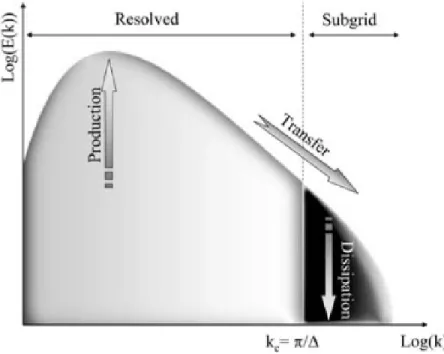
The transition of energy is shown in Figure 2.3 from right to left beginning with production, passing through the inertial subrange, then finally terminating with dissipation. Kolmogorov devised several hypotheses to support the energy cascade. First, the hypothesis of local isotropy in which the small scale turbulent motion (l << l0) are statistically isotropic [10, p.184]. To further define whether eddies are

considered isotropic, a separation length scale is defined as lEI ≈ 1₆l0. The region

above lEI is considered the energy containing range and below lEI the eddies are

considered locally isotropic [10, p.184]. The smallest turbulence scale,η, is defined as the Kolmogorov length scale which occurs when the Reynolds number based on the Kolomogorov length scale is exactly one [10, p.185]. Defining a length scalelDI = 60η

specifies a separation between viscosity dominated flow and inertial dominated flow [10, p.186]. This separation,lDI, outlines the maximum size of the dissipation range

energy in the small eddies to heat in the viscosity dominated region [10, p.186-187]. Conversely,lDI is the minimum of a region called the inertial subrange that is capped

bylEI where the viscous effects are negligible [10, p.186-187].

Figure 2.3: Eddy energy cascade (Figure from Pope [10, p.188])

2.2.3 Oil Flow Visualization. The use of oil flow visualization techniques are commonly applied to assess the fluid flow on the surface of an object [11]. The technique includes applying oil as a thin film, usually less than 1.27 millimeters, or as a dot matrix across the desired surface, then running the experiment allowing the patterns in the oil to develop [12]. The method can be applied to a wide range of flows from low speed water and wind tunnels to supersonic wind tunnels, with the

main consideration being the ratio of the viscosity of the fluid in the boundary layer to that of the oil, which for wind tunnels lies between 10−2 _{to 10}−4 _[12].

The main assumptions of oil flow visualization technique is that the oil streak-lines follow the streamstreak-lines of the flow near the surface and that the oil has negligible impact on the boundary layer flow [12]. Squire derived oil flow equations from the viscous equations of slow motion by assuming that the oil and the air share the same velocity and viscous stresses [12]. The primary parameter in resolving flow visual-izations with oil and the equations is the ratio of the viscosity of the fluid in the boundary layer to that of the oil [12]. Further testing by Squire showed the oil curves are not affected by the oil thickness, airflow speed, or velocity distributions [12]. Sep-arated regions in oil flow visualizations form an accumulation of oil upstream of the true separation point, this indication of separation can underestimate the separation distance by as much as 5% in compressible flows, but it can be less pronounced for turbulent flows than for laminar flows [12].

2.2.4 Separated Flow Topology. While the previous section discussed the methodology of oil flow visualizations, the interpretation of the surface patterns sur-rounding a separated regions and its translation into three-dimensions requires knowl-edge of the topology of the flows and the definition of standard terms. Oil flow visu-alizations resolve the skin friction lines of an experiment, and when the skin friction is exactly zero, singular points occur. Singular points can be classified into nodal points, sprial nodes (foci), or saddle points as presented in Figure 2.4 [13].

Nodal points are a singular point common to an infinite number of skin friction lines, and can be further classified into a nodal point of attachment or separation depending if the flow is away from the point or towards the point, respectively [13]. The nodal point displayed in Figure 2.4 is a nodal point of attachment. Spiral node is a point that has no common tangent line where the lines spiral around a point, and like the nodal point, can be points of attachment, as seen in Figure 2.4, or separation [11]. Lastly, the saddle point has only two lines that pass through it, one that is pointing into the point and one out of the point, the line created by these two act as a divider for all other skin friction lines that closely miss the singualar point [13]. Saddle points typically occur to separate nodal points of attachment [13].

Transitioning to three-dimensional flows, the stream surface is created by the projection of the lines passing through a saddle point and terminating at nodal points [13]. Steady state three-dimensional flows have geometries that appear to bifurcate along a stream surface, with the surface acting as a dividing surface just as the saddle point acts as a dividing line [13]. Positive bifurcations occur along a stagnation line, where negative bifurcations usually come from uplifting counter-rotating vorticies as shown in Figure 2.5 [14].

Figure 2.5: Stream surface bifurcations (Figure from Wellborn et al. [11])

A common way of presenting oil flow visualizations consists of mapping it on a “skeleton” drawing by cutting the S-duct along the upper surface centerline and unwrapping the oil flow visualization onto a flat horizontal surface with the bottom centerline in the middle of the figure [11]. The left hand side of Figure 2.6 shows the unwrapped lower region of a serpentine region that contains two saddle points and two spiral nodes along with both positive and negative bifurcation stream lines [11].

The pattern presented is common for separation regions and has been named “owl face” separation [15]. The right hand side of Figure 2.6 presents a more possible representation of the flow at a given snapshot because it is considered an impossible solution to have a single streakline passing through two saddles without a node in between them as it is unstable [15]. This more possible separation was justified by saying the unsteadiness causes oscillations between the spiral nodes and the saddles [15].

(a) Unstable (b) Stable

Figure 2.6: Stream surface bifurcations (Figure from Wellborn et al. [11])

Because of the lack of visible spiral node along the centerline, it is considered an “owl face of the first kind” which is displayed in three dimensions in Figure 2.7. The stream surfaces coil around the flow creating two tubes representing the two vortical structures that can be observed in the flow [13]. As the dividing surface rolls up around the vortical cores as it develops downstream, the well-defined core that results is called a vortex [13].

The diffusing serpentine pressure driven inlet is a viscosity dominated problem. The impact of viscosity on the development of the boundary later and effects in tur-bulence have been discussed in order to understand the physics that is being modeled. While oil flow visualizations of a wind tunnel will not be conducted in this study, the modeled solutions will produce surface streamlines that will be used to compare to oil flow visualizations previously completed, assisting with the determination of the location of separated flow.

Figure 2.7: Owl face of the first kind (Figure from Wellborn et al. [11])

2.3 Diffusing Serpentine Inlet Duct

The first application of a diffusing serpentine inlet duct was in the rear center tail engine of the Boeing 727, and the first studied S-ducts were conducted during the design [1]. Since then, this type of inlet has been used on General Dynamics F-16 and the McDonnell-Douglas F-18 [1]. Diffusing serpentine inlet ducts, like Figure 1.1, are dominated by compressible subsonic flow driven by the geometry of the inlet. S-duct geometry often results in flow separation and subsequent reattachment on the lower surface of the duct which will be further discussed in Section 2.3.2. Flow distortion detrimental to the turbine engine results from the separation bubbles within the duct and is discussed further in Section 2.3.3.

2.3.1 Geometry. At the core, diffusing serpentine inlet ducts, commonly referred to as S-ducts, contain an offset to the flow direction between the inflow and outflow. Serpentine inlet can contain a single turn (drop down) or double turn (drop down - rise up) S-duct as shown in Figure 2.8. Each turn can be broken down into two bends. In the case of the single turn S-duct, the first bend begins the transition downward and the second bend returns the flow direction to be parallel to the flow at the throat before the first bend. For a double S-duct the two bends within the first turn are identical to a single turn S-duct, and are reversed within the second

turn. Similarly, since the flow physics of the single are essentially experienced again within the second, so this section focuses on the flow within a single turn diffusing serpentine inlet duct. The diffusing inlet gradually and continuously increases in diameter throughout the serpentine inlet creating the diffusion required to decrease the flow velocity, preparing it for what would be a turbine engine compressor fan, while trying to minimize the flow distortion and total pressure loss [16, p.460].

Figure 2.8: Double S-duct comprised of two single S-ducts

2.3.2 Fluid Flow. The flow is dominated by the momentum of the inflow that upon reaching the first bend, overshoots the lower bend and is forced downward along the upper surface creating an adverse pressure gradient on the upper surface and a favorable pressure gradient on the lower surface [1]. This results with an increased pressure coefficient on the upper surface with decelerating flow, and a corresponding decrease in pressure coefficient on the lower surface with accelerating flow. Also affected by the redirection of the flow is the boundary layer thickness, which is the thinnest on the top and thickest on the bottom, being attributed to the axial pressure gradients with accelerated flow near the bottom and slower flow near the top [1].

The decrease in fluid in the lower portion of the inlet is replaced by pressure driven flow perpendicular to the serpentine centerline from the boundary layers to the lower surface centerline [1]. Fluid is continually moved from the boundary layer into the low momentum region along the bottom surface convecting the low momentum region higher in the duct, while developing and exciting the two counter-rotating vorticies [11]. Additionally, a local minimum of the total pressure is achieved in the duct [1].

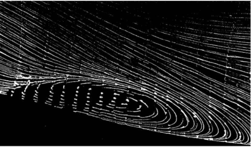
The separation in the bottom part of the duct is caused by a blockage of the flow creating a favorable pressure gradient, accelerating the flow into the second bend of the single turn S-duct. Even though the flow was separated, a noticeable increase in static pressure was caused by the continued diffusion of the duct [1]. Figure 2.9 shows the flow traveling from left to right through a single turn S-duct with oil flow visualizations along the center plane. The separated region continues in the bottom of the duct until the flow reattaches as the region of reversed flow thins resulting from the continuous inflow of boundary layer fluid [11]. At this point, the region of low momentum fluid is lifted off of the wall developing into a region of low velocity and low total pressure in the bottom half of the duct [11].

Figure 2.9: Oil flow visualization along a plate inserted along centerline plane within the single turn S-duct flow moving from left to right. (Figure from Well-born et al. [11])

In the second bend of the single turn S-duct, the cross-flow pressure gradient begins to reverse with boundary layer flow flowing towards the upper centerline [11]. Although this is a similar trend to the lower surface in first bend, no large scale vortical structures or flow separation occurs on the upper surface in the second bend because the pressure gradients and boundary layer flow is not as strong as in the first bend [11]. This is shown in Figure 2.9 with flow along the second bend on the upper surface being attached without the indication of recirculating flow.

In the case of the double, or two turn, S-duct, the flow features observed by Wellbornet al.[1] within the first two bends comprising the single S-duct are repeated within the second turn. The second turn within a double S-duct is an upward offset, as opposed to the downward offset in the single turn S-duct in Figure 2.9. The first turn will still contain the separation region on the bottom surface in the second bend, but the separation in the second bend of the second turn is now on the upper surface. Therefore, much of the same flow features observed in the single turn S-duct will be experienced twice within the double turn S-duct as the driving physics remains the same in both turns.

2.3.3 Flow Distortion. Vorticies within the flow create distortion of the flow by degrading the uniformity and the magnitude of the total pressure profile. The fully evolved pair of counter-rotating vortices in the lower half of the duct, like the vorticies within the owl face of the first kind in Figure 2.7, continue to move low momentum fluid towards the duct’s center extending above the centerline [11]. At this point the flow has returned to a downstream direction and the cross-stream static pressure gradients have subsided [1]. The difference in momentum in a cross-stream plane presents as a difference in velocity, each with an associated dynamic pressure. With a constant static pressure, the dynamic pressure variance across the plane results in a difference in total pressure across the plane. As the total pressure profile is not consistent across the plane, the flow is considered distorted. A simple calculation of

the inlet distortion is:

Inlet Distortion = (pt max−pt min) pt avg

(2.7)

where the difference in maximum and minimum total pressure, pt max and pt min, is

divided by the time averaged total pressure, pt avg [16, p.425]. When the maximum

and minimum total pressure values across the plane are the same, the inlet distortion would calculate results with the ideal value of zero. As the difference between the maximum and minimum total pressures increase, the inlet distortion also increases. The inlet distortion varies with mass flow rate and angle of attack, but a typical design point has an inlet distortion of less than 0.1 for a good inlet [17]. Increasing the angle of attack increases the inlet distortion as the flow is not perpendicular to the beginning of the duct [16]. For S-ducts, the increase of mass flow also increases the inlet distortion as the strength and size of the separated region increases [4]. Additionally, the total pressure of the flow is compared to the total pressure before the inlet in order to assess the total pressure recovery. The flow distortion resulting from a serpentine inlet lowers the engines surge line as in Figure 2.10, the line above which it is impossible to operate the engine without the possibility of damage to the engine and aircraft [16, p.164,425]. Further, the decrease in the surge line lowers the pressure ratios that can be obtained in turn lowering the possible thrust of the engine [16].

Formal definitions and methods of determining both circumferential and radial flow distortion are outlined by the Society of Automotive Engineers [19]. The defini-tion of circumferential distordefini-tion comes from the combinadefini-tion of intensity, extent, and multiple-per-revolution [19]. The intensity, or magnitude, of the distortion is the ratio of the value of the pressure defect for the ring divided by the face average pressure (∆P C/P), while the extent defines the portion of the ring that is below the average ring pressure [19]. Lastly, the multiple-per-revolution is the number of low pressure regions that exist around the ring [19]. The difference between the average pressure of a ring and the average pressure of the face (∆P R/P) defines the radial distortion of the ring, which can be positive or negative depending if the difference is above or below the face average respectively [19].

Diffusing serpentine inlet ducts have seen increased use since the first produc-tion applicaproduc-tion in the Boeing 727 as a means to locate the engine and inlet in more convenient locations. Although the number of different variations could be infinite, the general shape includes a duct that increases in cross sectional area while directing the flow downward then back. The fluid flow generally produces separated flow at the bottom part of the bend, which propagates into large counter-rotating vorticies that create flow distortion at the compressor plate. Inlet designers characterize the dis-tortion level to provide to the engine manufactures. In turn the engine manufactures determine if the level is acceptable for a particular engine. Different engines can have different levels that are determined “acceptable” and as such there is no definition of acceptable levels of distortion. The importance of this study is determining guidance to better predict the distortion observed for a given geometry based on modeling for implementation by inlet designers.

2.4 Reynolds Averaged Navier Stokes Turbulence Models

RANS turbulence models are commonly used for turbulent flows in CFD as they are computationally inexpensive compared methods like LES or DNS, resulting

from modeling rather than resolving the turbulent viscosity. This section lays out the assumptions, formulation, and limitations associated with RANS models.

2.4.1 Assumptions. In order to model the turbulence, RANS models solve for the Reynolds stress using the Boussinesq hypothesis for first order closures. The Reynolds stress is an additional term introduced by performing Reynolds or Farve averaging to the Navier-Stokes equations, resulting in a closure problem. The Boussi-nesq hypothesis is used to solve the closure problem and relates turbulent stresses as linearly proportional to mean strain rate via the eddy viscosity [20]. This rela-tion is dominated by the observarela-tion that momentum transfer within turbulent flow is primarely driven by mixing resulting from the large energetic eddies [20]. The Boussinesq hypothesis relationship for incompressible Reynolds averaged equations can be expressed as

τij = 2µTS¯ij−

2

3ρkδij (2.8) where τij is the Reynolds stress tensor, µT is the eddy viscosity, ¯Sij is the Reynolds

averaged strain rate tensor,k is the turbulent kinetic energy, andδij is the Kronecker

delta [20].

Another assumption commonly applied is Morkovin’s hypothesis. This hypoth-esis assumes that density fluctuations do not notably impact the turbulent boundary layer [20, p.220]. Morkovin’s hypothesis is not applicable to hypersonic flows, com-pressible free shear layers, or combustion flows with heat transfer [20, p.220]. Yet, this hypothesis is still used in these applications to make the problems more tractable.

2.4.2 Formulation. The RANS equations are arrived by averaging the Navier Stokes equations. The first method was proposed by Reynolds in 1895 and thus the basis of the name Reynolds-Averaged Navier-Stokes [20, p.217]. Reynolds averag-ing can be applied by decomposaverag-ing the governaverag-ing equations into mean and fluctuataverag-ing components, then solving for the mean component [20, p.217]. The breakdown into

the two components can be expressed as:

u=u+u0 (2.9)

where the bar denotes the mean component and the prime denotes the fluctuating component. This breakdown can be applied to each velocity component, density, and pressure. The mean component can be achieved by three different averages: a time average, spatial average, or ensemble average, and thus is applicable for stationary turbulence [20, p.217]. Spatial averaging occurs across a control volume and thus is appropriate for homogenous turbulence [20, p.217]. Lastly, ensemble average is applied by averaging across a number of samples, which lends itself useful for general turbulence [20, p.218].

A different approach to Reynolds averaging can be applied to situations when the density is not constant by applying Farve averaging to the Navier-Stokes equa-tions. This is of particular importance for flows where Morkovin’s hypothesis is not applicable, when performing a Reynolds average would produce additional unknown terms including a triple product, but Farve decomposition prevents these additional terms. The Farve averaging takes the form:

e u= ρu

ρ (2.10)

in which the tilde denotes the Farve averaged quantity and the bar represents averaged quantities.

The most common method is a combination of Reynolds averaging and Farve averaging to produce a model that is applicable to a wider range of flows. For this method, Reynolds averaging is applied to density and pressure, while all the remaining variables are Farve averaged for the compressible Navier-Stokes equations [20, p.220].

There are different types of first order RANS models including 0-equation, 1-equation, and 2-equation models. A 0-equation model such as Baldwin-Lomax model

is an algebraic model that does not solve for any additional transport. The most pop-ular 1-equation model is the Spalart-Allmaras model, and it solves for the transport equation for eddy viscosity coded into the equation for turbulent kinematic viscosity. The Spalart-Allmaras model reasonably models adverse pressure gradients and flow separation and is best suited for airfoil and wing applications [20, p.225]. k−solves for the transport of turbulent kinetic energy k and the turbulent dissipation rate , and while likely the most popular 2-equation turbulence model, it requires a damping function in order to stay valid throughout the viscous sublayer [20, p.228]. k−ω is very similar to k− except solving for the specific rate of dissipation ω=/k, which has better resolution near walls [10, p.383]. The Mentor SST model combines the two through a blending function to take advantage of the strengths by using k− away from the wall andk−ω near the wall.

For second order closures, the Boussinesq hypothesis is no longer assumed, which results in the addition of six additional unknown terms. Reynolds Stress models are a second order closure RANS models that solve for the six unknown terms though six additional equations. This method includes empirical relations but it includes advection/diffusion flow history, normal stresses that behave appropriately to sud-den changed in strain, and allows convection and production terms to respond to curvature, rotation, and stratification [20].

2.4.3 Limitations. There are several limitations to RANS models in addition to those previously listed for individual methods. First, RANS turbulence models have strict requirements for near wall spacing in order to accurately solve for the surface quantities and boundary layer. Typically, the first cell needs to have a height that is kept under one wall unit (y+ = 1) [8]. The small spacing restricts the maximum timestep, as defined from Von Neuman stability analysis, which in turn increases the number of iterations run to reach a solution increasing the computational cost, core hours, needed for the simulation. Additionally, the maximum Reynolds number for the problem is limited due to a decreasing boundary layer thickness for higher

Reynolds number flows driving the requirement for more cells near the wall increasing the memory requirement for simulations above resource limitations.

The basis of first order turbulence closures, the Boussinesq hypothesis, is also limited with its applications. Specifically, it looses validity for flows with significant streamline curvature, boundary layer separation and reattachment, sudden change of mean strain rate, rotation and stratification, and secondary flows in ducts [20, p.223]. As these are all flow features present in the S-duct, a RANS turbulence model would be a poor choice for modeling the flow.

This section provided a brief overview of RANS turbulence models, while there is much more on the topic, the main points relative to the current study were pre-sented. The assumptions allow for RANS models to resolve less of the turbulent eddies than LES or DNS, which allows for cheaper and faster computational simula-tions. Conversely, these assumptions come at a cost of lower fidelity and the potential for inaccurate solutions if applied incorrectly. Modifying the governing equations through Reynolds averaging, Farve averaging, or the combination of the two is core to the methodology of RANS methods, but each average has its uses and limitations. In regards to a diffusing S-duct, the limitations for RANS have thus far prevented accurate predictions of the flow distortion, total pressure recovery, and separation locations from a single model [3]. A more detailed discussion on recent applications of RANS models to the diffusing S-duct can be found in Section 2.7.

2.5 Large Eddy Simulation Turbulence Models

LES serves itself as a turbulence modeling alternative that is less cost prohibitive than DNS but can yield more accurate results than RANS models. DNS does not use a turbulence model and resolves all temporal and spatial scales with the turbulent flow. For this reason DNS requires cells on order of the Kolomogorov length scale and the time step to match the Kolomogorov time scale. The primary difference between DNS and LES is LES resolves turbulent energy containing scales that are larger than

a filtered size, usually on the order of the cell size, and models the scales smaller than the resolved scales using a sub-grid stress (SGS) model. The observation that small scales of turbulence are relatively isotropic allows for a simple SGS model to compute rather than fully resolving it making LES possible [21]. Energy containing turbulent eddies are eddies larger than 1/6 of the integral length scale, which provides a scale for the cell size [10, p.184]. For the S-duct in this study, this falls on the order of 10 to 100 micrometers. In order to compute appropriate wall shear and heat transfer for the boundary layer at the wall within a LES turbulence model, Wall-Resolved LES or Wall-Modeled LES can be applied to account for the boundary layer. Wall-Modeled LES can be classified as Hybrid RANS/LES method or Wall-stress model method [22].

2.5.1 Turbulence Scale Filtering. Defining the separation between resolved and modeled scales can be completed using either an explicit or implicit method. The explicit method uses a filtering equation like a tophat, sharp Fourier cut-off, or Gaussian filter to separate large and small scale turbulence [20, p.236-237]. Implicit turbulence scale separation can be achieved by allowing the scale of the grid size to be the filter [21]. Note that this implicit filtering is different than Implicit Large Eddy Simulation (ILES) which uses numerical dissipation within the model to act as a subgrid model without the use of an actual subgrid model [23]. While the implicit filtering is less computationally demanding by not needing additional equations, it requires a carefully constructed grid where all cells are roughly cubes of the same size [21]. The need for cubes stems from the fact that the smallest eddy that can fully be resolved by the cell must be larger than the cell, therefore, the largest dimension of the cube defines the scale that can be resolved. Defining isotropic turbulence scales as scales that are not the large energy containing scales and are on the order of less than 1/6 of the integral length scales, sets a maximum size that the cells must be to resolve the flow [10, p.184]. The size of the integral scale is specific to the generation of the turbulence and thus could have different sizes for different types of flow conditions and geometries. In the S-duct used in this study, the separation was considered to be