www.elsevier.com/locate/spa
Quasi-maximum likelihood estimation in GARCH
processes when some coefficients are equal to zero
Christian Francq
a, Jean-Michel Zakoian
b,∗aEQUIPPE-GREMARS, UFR MSES, Universit´e Lille 3, Domaine du Pont de bois, BP 60149, 59653 Villeneuve d’Ascq, Cedex, France
bEQUIPPE-GREMARS and CREST, 15 Boulevard G. P´eri, 92245 Malakoff, Cedex, France
Received 13 February 2006; received in revised form 8 December 2006; accepted 11 January 2007 Available online 21 January 2007
Abstract
The asymptotic distribution of the quasi-maximum likelihood (QML) estimator is established for generalized autoregressive conditional heteroskedastic (GARCH) processes, when the true parameter may have zero coefficients. This asymptotic distribution is the projection of a normal vector distribution onto a convex cone. The results are derived under mild conditions. For an important subclass of models, no moment condition is imposed on the GARCH process. The main practical implication of these results concerns the estimation of overidentified GARCH models.
c
2007 Elsevier B.V. All rights reserved. MSC:62M10; 62F12
Keywords: Boundary of the parameter space; Conditional heteroskedasticity; GARCH model; Quasi-maximum likelihood estimation; Non-normal asymptotic distribution
1. Introduction
Much attention has been given recently to the asymptotic properties of the quasi-maximum likelihood estimator (QMLE) in the context of GARCH processes. Whereas ARCH (AutoRegressive Conditionally Heteroskedastic) models were introduced by Engle in 1982 [11], and generalized by Bollerslev in 1986 [7], it took about twenty years to see the emergence
∗Corresponding address: CREST and Universit´e Lille 3, Statistics, 15 Boulevard G. P´eri, 92245 Malakoff, France.
Tel.: +33 141177666; fax: +33 141177725.
E-mail address:[email protected](J.-M. Zakoian).
0304-4149/$ - see front matter c2007 Elsevier B.V. All rights reserved.
of consistency and asymptotic normality results for the general GARCH model under weak assumptions. Recent references dealing with the QML estimation of general GARCH(p,q) are the dissertation by Boussama [9], the monograph by Straumann [25] and the papers by Berkes and Horv´ath [4,3], Berkes, Horv´ath and Kokoszka [5], Hall and Yao [14] for GARCH models with heavy tailed errors, and Francq and Zakoian [12] (hereafter FZ). Using the QMLE in the GARCH framework is beneficial for it is much less sensitive with respect to heavy tailed unconditional distributions than, for instance, the least-squares method. Other estimation procedures which are not demanding in terms of unconditional moments have recently been suggested by Horv´ath and Liese [15] and Ling [18]. See Straumann and Mikosch [26], Ling and McAleer [20] for related work. See Ling and McAleer [19], Giraitis, Leipus and Surgailis [13] for recent surveys on theoretical results for GARCH models.
The GARCH estimation theory however suffers the major weakness of excluding the presence of zero coefficients in the true parameter value. Indeed, one important difference between GARCH and other popular time series models, such as ARMA models, is that the admissible parameter space needs to be inequality restricted. The data generation mechanism requires the conditional variance to be always strictly positive, which is generally obtained by imposing a strictly positive intercept and non-negative GARCH coefficients in the conditional variance equation (see however Nelson and Cao [23] for weaker, but generally non-explicit, conditions). A key regularity condition, imposed by the above cited papers to establish the asymptotic normality, is that the true parameter must lie in the interior of the parameter space. For instance, it is easily seen that the QMLE is not asymptotically Gaussian if, for instance, a GARCH(p,q) model is estimated when the underlying process is a GARCH(p−1,q), or a GARCH(p,q−1) process. Our aim in this paper is to derive the asymptotic distribution of the QML estimator under, if possible, the same mild conditions as are employed when the parameter is in the interior of the parameter space. The quasi-likelihood will be approximated by a quadratic function, and the asymptotic distribution will be obtained as the projection of a normal vector onto a convex cone. A quadratic approximation to the objective function and its optimization on a convex cone have been used by Chernoff [10] and Andrews [1] among many others (see the latter paper for a list of references). To our knowledge, when the parameter is on the boundary, asymptotic results for the general GARCH(p,q), or even for the GARCH(1, 1), are not available in the literature. Partial results can be found in Andrews [1,2] and Jordan [16].
The article proceeds as follows. Section2 describes the estimation problem of concern and recalls results available whenθ0 is not on the boundary. Section3 establishes the asymptotic distribution of the QMLE whenθ0is on the boundary. For a large class of GARCH models, the results are obtained without moment assumptions on the observed process. Section4shows how to practically compute the asymptotic distribution. Proofs are relegated to anAppendix.
For a matrix Aof generic term A(i,j)we use the normkAk = P|
A(i,j)|. The spectral radius of a square matrixAis denoted byρ(A). The symbols→L and→P denote the convergences in distribution and in probability.
2. Assumptions and preliminary results
Consider the GARCH(p,q) model:
t = p htηt ht =ω0+ q X i=1 α0it−i2 + p X j=1 β0jht−j, ∀t∈Z (1)
where (ηt) is a sequence of iid random variables such that Eη2t = 1, ω0 > 0, α0i ≥
0 (i = 1, . . . ,q), β0j ≥ 0 (j = 1, . . . ,p). A strictly stationary solution (t) is called
non-anticipative if t is a measurable function of the ηt−i,i ≥ 0. Let (1, . . . , n) be a
realization of lengthn of a non-anticipative strictly stationary solution(t)to Model(1). The
vector of parameters isθ = (θ1, . . . , θp+q+1)0 = (ω, α1, . . . , αq, β1, . . . , βp)0 and it belongs to a parameter space Θ ⊂ (0,+∞)× [0,∞)p+q. The true parameter value is denoted by
θ0=(ω0, α01, . . . , α0q, β01, . . . , β0p)0∈Θ.
Bougerol and Picard [8] showed that a unique non-anticipative strictly stationary solution(t)
to Model(1)exists if and only if the sequence of matricesA0=(A0t)has a strictly negative top
Lyapunov exponent,γ (A0) <0, where
γ (A0)= lim
t→∞ a.s.
1
t logkA0tA0t−1. . .A01k,
k · kdenoting any norm on the space of the(p+q)×(p+q)matrices, and
A0t = α01η2t · · · α0qηt2 β01ηt2 · · · β0pη2t Iq−1 0 0 α01 · · · α0q β01 · · · β0p 0 Ip−1 0
withIkbeing thek×kidentity matrix.
Conditionally on initial values20, . . . , 12−q,σ˜2 0, . . . ,σ˜
2
1−p, the Gaussian quasi-likelihood is
given by Ln(θ)=Ln(θ;1, . . . , n)= n Y t=1 1 q 2πσ˜t2 exp − 2 t 2σ˜t2 , where theσ˜2
t are defined recursively, fort≥1, by
˜ σ2 t = ˜σt2(θ)=ω+ q X i=1 αit−i2 + p X j=1 βjσ˜t−2 j.
The parameter spaceΘ is a compact subset of[0,∞)p+q+1 that bounds the first component away from zero. We will also assume throughout thatΘ contains some hypercube of the form [ω, ω] × [0, ε]p+q, for someε >0 andω > ω >0.
A QMLE ofθis defined as any measurable solutionθˆnof
ˆ θn =arg max θ∈ΘLn(θ) =arg min θ∈Θ ˜ ln(θ), (2) where ˜l n(θ)=n−1 n X t=1 ˜ `t, and `˜t = ˜`t(θ)= ˜`t(θ;n, . . . , 1)= 2 t ˜ σ2 t +logσ˜t2.
Notice that `˜t may depend on the whole set of observations since it is customary to choose
the empirical mean of the squared observations for the initial values. An ergodic and stationary approximation(`t(θ))of the sequence (`˜t(θ))is obtained as follows. Under the condition A2
below, denote by σt2=σt2(θ) the strictly stationary, ergodic and non-anticipative solution of σ2 t =ω+ q X i=1 αit−i2 + p X j=1 βjσt−2 j, ∀t.
Note thatσt2(θ0)=ht. Let
ln(θ)=n−1 n X t=1 `t, and `t =`t(θ)=`t(θ;t, . . .)= 2 t σ2 t +logσt2. LetAθ(z)=Pq i=1αizi andBθ(z)=1− Pp j=1βjzj. By convention,Aθ(z)=0 ifq =0 and Bθ(z)=1 ifp=0. To obtain the asymptotic properties of the QMLE in the classical case where
θ0is not on the boundary, the following assumptions can be made. A1: θ0∈
◦
Θ, whereΘ◦ denotes the interior ofΘ. A2: γ (A0) <0 andPpj=1βj <1,∀θ∈Θ.
A3: η2t has a non-degenerate distribution withEη2t =1.
A4: ifp>0,Aθ0(z)andBθ0(z)have no common root,Aθ0(1)6=0, andα0q+β0p6=0.
A5: κη:= Eη4t <∞.
It is worth noting that, in A2, the strict stationarity condition is imposed on the true value only. Forθ 6=θ0we only require the weaker condition thatPp
j=1βj <1 (see e.g. Kazakeviˇcius and Leipus [17], Th. 2.2). One important consequence ofγ (A0) < 0 is that Et2s < ∞for some s ∈ (0,1). For a proof of this statement see Nelson [22] and Berkes et al. [5, Lemma 2.3]. For detailed comments on these assumptions, and comparisons with similar conditions given in the aforementioned papers, see FZ, in which the following result is established.
Theorem 1.Let(θˆn)be a sequence of QML estimators satisfying(2). Then
(i) if A2–A4hold, almost surelyθˆn→θ0, as n→ ∞, (ii) if A1–A5hold,√n(θˆn−θ0) L →N(0, (κη−1)J−1), where J :=Eθ0 1 σ4 t(θ0) ∂σ2 t(θ0) ∂θ ∂σ2 t (θ0) ∂θ0 . (3)
In the next section we will allow true parameter values belonging to∂Θ := {θ0 ∈Θ :θ0i =0, for somei >0}. To preventθ0from reaching the upper bound ofΘwe defineθ0(ε)as the vector obtained by replacing all zero coefficients ofθ0byεand we make the following assumption. A6: θ0(ε)∈
◦
Θ for someε >0.
For instance, if the parameter space is specified asΘ = [ω, ω] × [0, α1] × · · · × [0, αq] ×
[0, β1] × · · · × [0, βp], Assumption A6 is satisfied whenω > ω0> ω >0 and 0≤θ0 < θ :=
(ω, α1, . . . , βp)0.
3. Asymptotic distribution ofθˆnwhenθ0is on the boundary
It is easy to understand why the positivity condition, namely α0i > 0 (i = 1, . . . ,q),
a Gaussian asymptotic distribution for √n(θˆn −θ0) is precluded when the components θˆi n
of θˆn are constrained to be non-negative and θ0 ∈ ∂Θ. If, for instance, θ0i = 0 then
√
n(θˆi n−θ0i) =
√
nθˆi n ≥ 0 for alln and the asymptotic distribution of this variable cannot
be a standard Gaussian.
ByTheorem 1, no moment assumption is required for the asymptotic distribution to hold, and thus for the existence of J, whenθ0is an interior point ofΘ. Whenθ0 ∈ ∂Θ, the asymptotic distribution of√n(θˆ
n−θ0)will to be seen to rely on the existence ofJas well. Before deriving this asymptotic distribution, we give an example showing that the matrix J may not exist if
Eθ0t4= ∞and A1 is relaxed.
3.1. Possible non-existence of J under A2–A5
Consider the ARCH(2) modelt = σtηt,σt2 = ω0+α01t2−1+α02 2
t−2 whereω0 > 0,
α01≥0,α02=0, and the distribution of the iid sequence(ηt)is defined, fora >1, by P(ηt =a)=P(ηt = −a)=
1
2a2, P(ηt =0)=1− 1
a2.
This ARCH(2) model is used to generate the quasi-likelihood function but t is in fact an
ARCH(1). The strict stationarity conditionγ (A0) < 0 takes the formα01 <exp−E(logηt2)
for an ARCH(1). The process (t) is therefore strictly stationary for any value of α01 since exp−E(logη2t) = +∞. Howevert is not second-order stationary whenα01≥1.
We have 1 σ2 t ∂σ2 t ∂α2(θ 0)= 2 t−2 ω0+α01t2−1 , whence Eθ0 1 σ2 t ∂σ2 t ∂α2 (θ0) 2 ≥ Eθ0 ( 2 t−2 ω0+α01t−2 1 )2 ηt−1=0 P(ηt−1=0) = 1 ω2 0 1− 1 a2 Eθ0(t−4 2)
firstly becauseηt−1 =0 entailst−1=0 and secondly becauseηt−1andt−2are independent. It follows that Jdoes not exist ifEθ04t = ∞.
3.2. Assumptions and main result
It is then clear that the assumptions ofTheorem 1are not sufficient to ensure the existence of
J when A1 is relaxed. In view of these remarks we introduce two alternative assumptions. The first one is a moment condition.
A7: Eθ0t6<∞.
In many interesting cases, except the ARCH(q)models, no moment assumption ont2will be required. Indeed, it will be sufficient to ensure the existence of moments for the score vector normalized by σt2. Note that under the condition γ (A0) < 0, the strictly stationary solution
σ2
t(θ0)has an expansion of the form: σt2(θ0) = c0+P∞j=1b0j2t−j withc0 > 0, b0j ≥ 0.
moments of{∂σt2/∂θ}/σt2will rely on the fact that every termt2−j appearing in the numerator of this ratio is also present in the denominator. We therefore consider the assumption
A8: b0j >0 for all j≥1, whereσt2(θ0)=c0+P∞j=1b0jt−2 j.
It should be noted that a simple sufficient condition for A8 isα01 >0 andβ01 > 0 (because
b0j ≥ α01β01j−1). A necessary condition is obviously thatα01 >0 (becauseb01 =α01). More generally, a necessary and sufficient condition for A8 is
{j|β0,j >0} 6=∅ and
j0 Y
i=1
α0i >0 for j0=min{j |β0,j >0}, (4)
meaning that the ARCH coefficients αcannot cancel up to the order j0 of the first GARCH coefficientβ equal to zero. Assumption A8 does not apply to ARCH(q) models, which is not surprising in view of the example in Section3.1. The main result of this section is the following.
Theorem 2.Let (θˆn) be a sequence of QML estimators satisfying (2). Then if A2–A6 and
eitherA7orA8hold, √ n(θˆn−θ0) L →λΛ:=arg inf λ∈Λ {λ−Z}0J{λ−Z}, with Z∼N(0, (κη−1)J−1), Λ=Λ(θ0)=Λ1× · · · ×Λp+q+1,
whereΛ1=R, and, for i=2, . . . ,p+q+1,Λi =Rif θ0i 6=0andΛi = [0,∞)if θ0i =0.
In the ARCH case, the result can be stated as follows.
Corollary 3. Let p = 0and let (θˆn)be a sequence of QML estimators satisfying(2). Then if
γ (A0) <0,A3, andA5–A7hold, √ n(θˆn−θ0) L →λΛ:=arg inf λ∈Λ {λ−Z}0J{λ−Z}, with Z∼N(0, (κη−1)J−1), Λ=Λ(θ0)=Λ1× · · · ×Λq+1,
whereΛ1=R, and, for i=2, . . . ,q+1,Λi =Rif θ0i 6=0andΛi = [0,∞)if θ0i =0. Comments.
1. Forθ0 ∈
◦
Θ, the result of this theorem reduces to that of Theorem 1. Indeed, in this case
Λ=Rp+q+1andλΛ=Z ∼N 0, (κη−1)J−1. Hence,Theorem 2has interest only whenθ0 belongs to∂Θ.
2. We stress the fact that the moment condition A3 is on the iid process, not on(t). For values
ofθ0satisfying A8, the asymptotic distribution is derived under the same mild conditions as are employed for the standard case whereθ0∈
◦ Θ.
3. Andrews [1] considered, as an example of a more general framework, the case of a GARCH(1,q)model withq > 1, assuming that the parametersα1 andβ1 are bounded away from zero. Hence the case whenα01orβ01are on the boundary is not covered. In particular, this precludes the ARCH(q) and the GARCH(1, 1) models with coefficients equal to zero. Jordan [16] allows a parameter belonging to the boundary of a non-compact set, but is restricted to an ARCH framework and requires the moment assumptionEt8<∞.
4. Practical derivation of the limiting distribution
The vectorλΛappears to be the orthogonal projection of Z ontoΛ, where orthogonality is defined in the metric associated with the covariance structure J (see the proof of Lemma 13 below), namelyx⊥yiffx0J y = 0. It is uniquely determined becauseΛ is convex. Moreover, the fact thatΛis a convex cone whose faces are sections of subspaces allows one to obtain this projection in a more explicit way (see e.g. Perlman [24]). Suppose, without loss of generality, that the first d1 components ofθ0 are positive, and that the lastd2components are null, with
d1+d2 = p+q +1. We have Λ = Rd1 × [0,∞)d2 = {λ ∈ Rd1+d2 | Kλ ≥ 0}, where
K =(0d2×d1,Id2). LetK={K1, . . . , K2d2−1 , where theKiare matrices obtained by cancelling 0, 1 or several (up tod2−1) rows ofK. LetMi =Ki0 KiJ−1Ki0
−1
Ki, letPi =Id1+d2−J −1M
i
and denote byλKi =PiZthe projection ofZonto the linear subspace ofR
d1+d2 spanned by one
of the 2d2−1 faces ofΛ(including the “face”
Rd1× {0}d2), defined byKiλ=0. Then we have,
withC= {λK i :Ki ∈KandKλKi ≥0}, λΛ = Z1 Λ(Z)+1Λc(Z)×arg min λ∈C kλ−ZkJ = Z1Λ(Z)+ 2d2−1 X i=1 PiZ1Di(Z), (5)
for some partition(Di)ofRd−Λ.
For the sake of illustration we consider the following examples.
Example 4 (One Zero Coefficient). Suppose that only one component of θ0 is zero, the other
components being positive. Thusd2=1,Λ=Rd1× [0,∞),K =(0, . . . ,0,1),K= {K}, and,
lettingZ =(Z1, . . . ,Zd)0, λΛ=Z1 Zd≥0+P Z1Zd<0, P=Id−J −1K0( K J−1K0)−1K. It follows that λΛ=Z−Z− dc (6)
where Zd− = Zd1Zd<0, andc = E(ZdZ)/Var(Zd)is the last column of J
−1 divided by the (d,d)-element of this matrix. Note that the last component ofλΛis Zd+ := Zd1Zd>0. Letting λΛ=(λΛ
1, . . . , λ
Λ d)
0, it is also seen thatλΛ
i =Ziif and only if Cov(Zi,Zd)=0.
Example 5 (Noise Estimated as an ARCH(1)). To be more specific, consider Example 4with
d1(=d2)=1. Thenθ0=(ω0,0)0and J =Eθ0 1 σ4 t 1 t2−1 2 t−1 t4−1 = 1 ω2 0 1 ω0 ω0 ω20κη , J−1= 1 κη−1 ω2 0κη −ω0 −ω0 1 . Thus λΛ=Z−Z− 2 −ω0 1 = Z1+ω0Z−2 Z2+ .
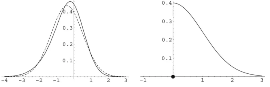
Fig. 1. Asymptotic marginal distributions of the QMLE, for the ARCH(1) modelt =
q ω+α2
t−1ηt withω0= 1, α0=0 andκη=1.5. The left-hand graph displays, as a full line, the density ofλΛ1, and as a dotted line the density of the normal distribution with the same first and second moments. The right-hand graph displays the distribution ofλΛ2, with the Dirac mass 1/2 at 0 and the densityN(0,1)on(0,+∞).
Straightforward computations show thatEλΛ1 = −ω0Eλ2Λ= −ω0(2π)−1/2and Var(λΛ)= 1 2 1− 1 π 1+(1−2κη)π 1−π ω 2 0 −ω0 −ω0 1 .
It can be seen that Var(λΛ1)=ω2 0κη−
1 2(1+
1
π)ω20 <Var(Z1)=ω02κη (seeExample 6below for a generalization).Fig. 1displays the density ofλΛ1 and that of the continuous part ofλΛ2. It is interesting to note that even the first component ofλΛis not Gaussian. Elementary computations show that its skewness coefficient is given by
E λΛ1 −EλΛ13 VarλΛ13/2 = −1 2− 1 π 1 √ 2π n κη−1 2 1+π1o 3/2.
Note that this skewness is always negative but vanishes whenκηgoes to infinity.
Example 6(Asymptotic Mean Squared Error Comparisons). The results of Lovell and
Prescott [21] for the Gaussian multiple regression model show that the Mean Squared Error (MSE) of the least-squares estimator subject to a positivity constraint is smaller than the conventional (unconstrained) MSE. As noted by Andrews [2], this property is probably true for non-standard models with a parameter on the boundary of a convex set, but this property remains a conjecture. We will verify this conjecture onExample 4. In view of(6), we have
MSE(λΛ):= Var(λΛ)+EλΛEλΛ0 = Var(Z)+Var(Zd−)cc0−2E(Z−dZ)c0+(E Zd−)2cc0. SinceE Zd−Z = E Zd+Z = E ZdZ/2 =Var(Zd)c/2, E Zd− = − √ Var(Zd)/2π andE(Zd−)2 = Var(Zd)/2, we have
MSE(λΛ)−MSE(Z)= {E(Zd−)2−Var(Zd)}cc0= −
Var(Zd)
2 cc
0
(7)
showing that the difference MSE(λΛ)−MSE(Z) is a semi-negative definite matrix. Thus, when one GARCH coefficient is null, the conventional asymptotic standard errors for the QML
estimators of the other coefficients are too large. This may have consequences in practical applications.
Acknowledgements
The authors are grateful to Professor B.P. P¨otscher who gave us helpful comments on the preliminary version of this paper which was presented at the ESEM-EEA 2006 congress. The authors are also very grateful to the Editor and the referees for their comments and constructive suggestions.
Appendix A. Proofs and technical results
A.1. Asymptotic normality of the normalized score
Before proving Theorem 2 we will establish several lemmas. Note that when θ0 ∈ ∂Θ, the functionσt2(θ)may be negative in a neighborhood ofθ0and`t(θ)may be non-defined in
this neighborhood. Instead of a standard Taylor expansion, we will use a one-sided expansion, based on right derivatives of ln(θ) = n−1Ptn=1`t(θ) about θ0. For ease of notation, denote by ∂σt2(θ0)/∂θ := ∂σt2(θ0)/∂θi
i=1,...,p+q+1 and∂`t(θ0)/∂θ := (∂`t(θ0)/∂θi)i=1,...,p+q+1 the vectors of partial derivatives of σt and `t at θ0 with the i-th derivative replaced by the right derivative when θ0i = 0. We use the same convention for the derivatives of ln, `˜t
and˜ln at θ0, and for the second partial derivatives. Under this convention, the derivatives of
`t(θ)=2t/σt2+logσt2are given by
∂`t(θ) ∂θ = 1− 2 t σ2 t 1 σ2 t ∂σ2 t ∂θ , ∂2` t(θ) ∂θ∂θ0 = 1− 2 t σ2 t 1 σ2 t ∂2σ2 t ∂θ∂θ0 + 2 2 t σ2 t −1 1 σ2 t ∂σ2 t ∂θ 1 σ2 t ∂σ2 t ∂θ0 . (A.1) FZ [12] introduce the following notation forσt2and its derivatives:
σ2 t = ∞ X k=0 Bk(1,1) ω+ q X i=1 αit−k−i2 ! , (A.2) ∂σ2 t ∂ω = ∞ X k=0 Bk(1,1), ∂σ 2 t ∂αi = ∞ X k=0 Bk(1,1)t−k−i2 , (A.3) ∂σ2 t ∂βj = ∞ X k=1 Bk,j(1,1) ω+ q X i=1 αit2−k−i ! (A.4) where Bk,j =∂ Bk ∂βj = k X m=1 Bm−1B(j)Bk−m, B = β1 β2 · · · βp 1 0 · · · 0 ... 0 · · · 1 0 , (A.5)
andB(j)is a p×pmatrix with(1,j)th element 1, and all other elements equal to zero. Similar formulas, given below, hold for the second derivatives. Elementary properties of the matrixBare established in the following lemma.
Lemma 7. For j=1, . . . ,p
B(j)Bk ≤ Bk−j+1, for all k≥ j−1, (A.6)
B(j)Bk =B(j−k), for all0≤k< j, (A.7)
A B(1)≤ A, and for j6=`2, {A B(j)}(`1, `2)=0, ∀A≥0, (A.8)
B(1)B(j)=B(j), and B(i)B(j)=0, for i>1, (A.9)
Bk(1,1)≥βjBk−j(1,1), for all k≥ j. (A.10)
Proof. First note that, when j ≤ p, the j-th row of Bj is the first row of B. The first row of
B(j)A is the j-th row of A, and the other elements of B(j)A are zeros. Thus B(j)Bj ≤ B. Multiplying the two sides of the previous inequality byBk−j, whose elements are non-negative, yields (A.6). For k < j ≤ p, the j-th row of Bk is null, except one “1” in the j-th position, which shows(A.7). The j-th column of A B(j) is the first column ofA, and the other elements of A B(j) are zeros. Thus(A.8)and(A.9)are obvious. Inequality(A.10)comes from
Bk(1,1)=Pp
j=1βjBk−1(j,1)≥βjBk−1(j,1)=βjBk−j(1,1).
The second lemma allows to consider theL1norms of the derivatives ofσt2atθ0.
Lemma 8. Under the assumptions of Theorem2,
Eθ0 1 σ2 t ∂σ2 t ∂θ (θ0) < ∞, Eθ0 1 σ4 t ∂σ2 t ∂θ ∂σ2 t ∂θ0(θ0) < ∞, Eθ0 1 σ2 t ∂2σ2 t ∂θ∂θ0(θ0) < ∞.
Proof. In this proof and the subsequent ones,K andρ denote generic constants, whose values
might change from line to line but always satisfyK >0 and 0< ρ <1. Sinceσt−2is bounded by 1/ω, the proof ofLemma 8is straightforward under Assumption A7.
Now assume that, A8, instead of A7, holds. By(A.3),∂σt2(θ0)/∂ωis bounded sinceP∞k=0Bk is finite under A2. Sinceσt2(θ0)≥ω0>0,{∂σt2(θ0)/∂ω}/σt2(θ0)therefore possesses moments of any order. Consider the derivatives with respect toαi. LetB0be the matrixBforθ=θ0. We have, in view of(A.2),
σ2 t(θ0)=ω0 ∞ X k=0 B0k(1,1)+ ∞ X k=1 k X `=1 α0`B0k−`(1,1)t2−k
with by conventionα0` =0 when`6∈ {1, . . . ,q}. By assumption A8, for allk >0 there exists an integerik ∈ {1, . . . ,min(q,k)}such that
k X `=1 α0`B0k−`(1,1)≥α0ikB k−ik 0 (1,1)≥αB k−ik 0 (1,1) >0, (A.11)
for some positive constantα(one can take α = min{α0i : α0i 6= 0}). It follows that for any
s∈(0,1), in view of(A.2)and(A.3), 1 σ2 t ∂σ2 t ∂αi (θ0)= ∞ P k=0 B0k(1,1)t−i2 −k ∞ P k=0 B0k(1,1) ω0+ q P j=1 α0jt−2 j−k ! ≤ ∞ X k=i B0k−i(1,1)t2−k ω0+αB0k−ik(1,1)2t−k ≤ ∞ X k=i B0k−i(1,1)t2−ks ωs 0α1−s{B k−ik 0 (1,1)}1−s , (A.12) where the last inequality follows fromax/(b+cx)≤ axs/(bsc1−s)for alla,x ≥0,b,c>0 ands ∈ (0,1). The latter inequality comes from the elementary inequalityx/(1+x)≤ xs for allx≥0 and alls∈(0,1). Now, for any fixeds∈(0,1), we will show that
B0k−i(1,1)/{Bk−ik
0 (1,1)}
1−s ≤Kρk for allk. (A.13)
By A2 and the compactness ofΘ, we have supθ∈Θρ(B) <1. ThuskB0kk ≤ Kρk for allk, and sinceik belongs to the finite set{1, . . . ,q}, we have
n
Bk−ik
0 (1,1)
os
≤ Kρk, and it suffices to show that B0k−i(1,1)/Bk−ik
0 (1,1)is bounded by a constant independent ofk. It is sufficient to considerksuch that B0k−i(1,1)6= 0. Let j0be defined by(4)and letri ∈ {1, . . . ,j0}be such thati −1 ≡ ri −1 (mod j0), that isi = qij0+ri withqi ≥ 0. In view of(A.10), we have
Bk−ri 0 (1,1)= B k−i+qij0 0 (1,1)≥β qi 0j0B k−i
0 (1,1) >0. Moreover,α0ri 6=0 by(4). Thus one can
takeik =ri in(A.11), so that we have B0k−i(1,1)/Bk−ik
0 (1,1)≤1/β
qi
0j0, (A.14)
and thus(A.13)holds. Then(A.12)gives
Eθ0 1 σ2 t ∂σ2 t ∂αi (θ0)≤K (∞ X k=1 ρk ) Eθ0t2s. (A.15)
Sincet2has a moment of orders, for somes ∈(0,1), the right-hand side in the last inequality is finite. Henceσt−2(∂σt2/∂αi)has a moment of order 1 atθ=θ0.
Let us turn to the derivatives with respect toβj. In view of(A.4)we have
∂σ2 t(θ0) ∂βj =ω0 ∞ X k=0 Bk,j(1,1)+ ∞ X k=2 k X `=1 α0`Bk−`,j(1,1)t−k2 (A.16)
whereB0,j =0 and, fork>0, the matricesBk,j defined in(A.5)are taken atθ0. We obtain, for any 0≤`≤k−j, by(A.6)and(A.7),
Bk−`,j ≤ k−`−j X m=1 B0m−1B0k−`−m−j+1+ k−` X m=k−`−j+1 B0m−1B(j−k+`+m) =(k−`− j)B0k−`−j+ k−` X m=k−`−j+1 B0m−1B(j−k+`+m),
which, together with(A.8), entails that Bk−`,j(1,1)≤ (k−`− j)Bk−` −j 0 (1,1)+B k−`−j 0 (1,1) ≤ k B0k−`−j(1,1). (A.17) Fork−j < `≤kwe similarly obtain
Bk−`,j ≤ k−`
X
m=1
B0m−1B(j−k+`+m), and thusBk−`,j(1,1)=0. (A.18)
Therefore, from(A.16)we deduce
∂σ2 t (θ0) ∂βj ≤ω0 ∞ X k=j k B0k−j(1,1)+ ∞ X k=j+1 k−j X `=1 α0`k B0k−`−j(1,1)t−k2 . Hence, proceeding as in(A.12)we get
1 σ2 t ∂σ2 t ∂βj (θ0)≤K+ ∞ X k=j+1 k−j X `=1 α0`k B0k−`−j(1,1)t−k2s ωs 0α1−s{B k−ik 0 (1,1)}1−s , (A.19) and thus Eθ0 1 σ2 t ∂σ2 t ∂βj (θ0)≤K+K (∞ X k=1 kρks ) Eθ02ts <∞, (A.20) by arguments already used for (A.15). This allows to conclude that the first expectation in Lemma 8exists. Applying the H¨older inequality in(A.12)and(A.19)withssuch thatEt4s <∞, it can be shown that kσt−2∂σt2(θ0)/∂θk2 < ∞. Thus the second expectation in Lemma 8 exists.
Let us now turn to the second-order derivatives ofσt2. It follows from(A.3)that
∂2σ2 t ∂ω2 = ∂2σ2 t ∂ω∂αi =0 and ∂ 2σ2 t ∂ω∂βj = ∞ X k=1 Bk,j(1,1). Thus∂2σt2/∂ω∂βj ≤P∞k=jk B k−j
0 (1,1) <∞, by(A.17)and(A.18)with`=0, which proves that∂2σt2(θ0)/∂ω∂θi is bounded and admits moments at any order. The same conclusion holds
for∂2σt2(θ0)/∂ω∂θi /σt2(θ0). By(A.3)and(A.4)we find
∂2σ2 t ∂αi∂αj =0 and ∂ 2σ2 t ∂αi∂βj = ∞ X k=2 Bk−i,j(1,1)t−k2 ,
and the arguments used for the first-order derivative with respect to βj prove that
∂2σ2
t (θ0)/∂αi∂θ /σt2(θ0)is integrable. Differentiating(A.16)with respect toβj0gives
∂2σ2 t ∂βj∂βj0 =ω0 ∞ X k=0 Bk,j,j0(1,1)+ ∞ X k=2 k X `=1 α0`Bk−`,j,j0(1,1)2 t−k (A.21) where
Bk,j,j0 = ∂ Bk,j ∂βj0 = k X m=1 Bm−1,j0B(j)Bk−m 0 + k X m=1 B0m−1B(j)Bk−m,j0 := Bk(1,)j,j0 +B( 2) k,j,j0.
We first give a bound for the terms of the formB(j)Bk,j0involved inB(2)
k,j,j0. First note that when k ≤ p, only the firstkrows of B0k contain terms depending on theβj. Thus the last p−k+1
rows ofBk,j0 are equal to zero, and it follows that
B(j)Bk,j0 =0 fork< j. (A.22)
Using successively(A.7),(A.6)and(A.9), we obtain, for j,j0=1, . . . ,pandk>0,
B(j)Bk,j0 = k X n=1 B(j)B0n−1B(j0)B0k−n ≤ j X n=1 B(j−n+1)B(j0)B0k−n+ k X n=j+1 B0n−jB(j0)B0k−n = B(j0)B0k−j+ k X n=j+1 B0n−jB(j0)B0k−n,
where by convention B0k = B(k+1) = 0 fork < 0 andPk0
n=kxn = 0 fork > k0. Using again
(A.7)and(A.6), we obtain
B(j)Bk,j0 ≤ B(j+j 0 −k)+ k X n=j+1 B0n−jB(j0−k+n) for j≤k< j+j0, (A.23) B(j)Bk,j0 = B(j 0) B0k−j+ k−j0 X n=j+1 B0n−jB(j0)B0k−n+ k X n=k−j0+1 B0n−jB(j0)B0k−n ≤ (k− j0− j+1)Bk−j−j 0+ 1 0 + k X n=k−j0+1 B0n−jB(j0−k+n), k≥ j+j0. (A.24) From (A.22) we obtain Bk(2,)j,j0 :=
Pk
m=1Bm− 1
0 B(j)Bk−m,j0 = 0 fork ≤ j. Using the fact
that the first column of B(j) is null for j > 1,(A.22)and(A.23)entail Bk(2,)j,j0(1,1) = 0 for j ≤k< j+j0. With the same argument,(A.22)–(A.24)show that fork≥ j+j0
Bk(2,)j,j0(1,1)= k−j−j0 X m=1 B0m−1B(j)Bk−m,j0(1,1) ≤ k−j−j0 X m=1 (k−m−j0−j+1)Bk−j−j 0 0 (1,1) ≤ (k−j− j 0)(k−j− j0+1) 2 B k−j−j0 0 (1,1)≤k 2Bk−j−j0 0 (1,1).
Similarly we haveBk(1,)j,j0(1,1)≤k2B k−j−j0
0 (1,1). Therefore, from(A.21)we deduce
∂σ2 t ∂βj∂β0j (θ0)≤2ω0 ∞ X k=j+j0 k2Bk−j−j 0 0 (1,1)+2 ∞ X k=j+j0+1 k−j−j0 X `=1 α0`k2Bk−` −j−j0 0 (1,1) 2 t−k.
By the arguments used to show(A.20), we conclude that
Eθ0 1 σ2 t ∂2σ2 t ∂βj∂βj0(θ0) < ∞,
which shows the existence of the last expectation inLemma 8.
The following two lemmas show the existence of the information matrixJdefined in(3), under the assumptions ofTheorem 2.
Lemma 9. Under the assumptions of Theorem2,
Eθ0 ∂`t(θ0) ∂θ ∂`t(θ0) ∂θ0 < ∞ and Eθ0 ∂2` t(θ0) ∂θ∂θ0 < ∞.
Proof. In view ofLemma 8, the derivatives ofσt2divided byσt2possess second-order moments. Forθ = θ0, the variablet2/σt2 = η2
t possesses a first-order moment and is independent of
the terms involvingσt2and its derivatives. The results then follow from(A.1), using the H¨older inequality.
Lemma 10. Under the assumptions of Theorem2,
J is non-singular and Varθ0
∂`
t(θ0)
∂θ
=κη−1 J.
Proof. The proof follows fromLemma 9 and the identifiability assumptions A3, A4 (see FZ,
Proof of Theorem 2.2(ii)).
The following lemma, together withTheorem 1(i), readily shows that J can be consistently estimated byJˆ:=∂2ln(θˆn)/∂θ∂θ0.
Lemma 11. Under the assumptions of Theorem2, for anyε > 0, there exists a neighborhood
V(θ0)of θ0such that, almost surely,
Eθ0 sup θ∈V(θ0)∩Θ ∂2` t(θ) ∂θ∂θ0 < ∞ (A.25) and lim n→∞ 1 n n X t=1 sup θ∈V(θ0)∩Θ ∂2` t(θ) ∂θ∂θ0 − ∂2` t(θ0) ∂θ∂θ0 ≤ε. (A.26)
Proof. When A7 is assumed,(A.25)is a consequence of(A.1). Now assume that A8, instead of
be the integer defined in(4). LetV(θ0)be a neighborhood ofθ0such that inf θ∈V(θ0) j0 Y i=1 αi >0 and inf θ∈V(θ0) βj0 >0.
For the sequence(ik)= (ik(θ0))satisfying(A.11)and someα >0 (for instance one can take
α=infθ∈V(θ0)min{i:1≤i≤j0}αi), we have
inf θ∈V(θ0) αikB k−ik(1,1)≥α inf θ∈V(θ0) Bk−ik(1,1) >0.
Like for(A.12)we then have sup θ∈V(θ0) 1 σ2 t ∂σ2 t (θ0) ∂αi ≤K ∞ X k=i sup θ∈V(θ0) Bk−i(1,1) Bk−ik(1,1) ρk2s t−k, (A.27) using supθ∈V(θ 0)kB
kk ≤ Kρk, which is a consequence of sup
θ∈Θρ(B) < 1. Note that Bk−ik
0 (1,1) 6= 0 implies Bk−ik(1,1) 6= 0 inV(θ0), but that B
k−i
0 (1,1) = 0 does not imply
Bk−i(1,1)=0 inV(θ0). However, in any case we have
Bk−i(1,1) Bk−ik(1,1) ≤ 1 βqi j0 .
Indeed the last equality is straightforward whenBk−i(1,1)=0 and follows from(A.14)when
Bk−i(1,1)6=0. It follows that the sup inside the sum in(A.27)is bounded. Therefore
sup θ∈V(θ0) 1 σ2 t ∂σ2 t(θ0) ∂αi 3 <∞.
Similar existence of moments can be shown for the other derivatives involved in the second derivative of`t(θ).(A.25)follows.
Now, under A7 or A8, the ergodic theorem shows that
lim n→∞ 1 n n X t=1 sup θ∈V(θ0)∩Θ ∂2` t(θ) ∂θ∂θ0 − ∂2` t(θ0) ∂θ∂θ0 =Eθ0 sup θ∈V(θ0)∩Θ ∂2` t(θ) ∂θ∂θ0 − ∂2` t(θ0) ∂θ∂θ0 .
This expectation decreases to 0 when the neighborhoodV(θ0)decreases to the singleton{θ0}. Thus(A.26)is also proved.
The following lemma shows that the initial values are asymptotically negligible.
Lemma 12. Under the assumptions of Theorem2,
n−1/2 n X t=1 ( ∂`t(θ0) ∂θ − ∂`˜ t(θ0) ∂θ ) →0 (A.28) and sup θ∈V(θ0)∩Θ n−1 n X t=1 ( ∂2` t(θ) ∂θ∂θ0 − ∂2`˜ t(θ) ∂θ∂θ0 ) P →0. (A.29)
Proof. From FZ, p. 625, we have sup θ∈V(θ0)∩Θ n−1 n X t=1 ( ∂2` t(θ) ∂θi∂θj −∂ 2`˜ t(θ) ∂θi∂θj ) ≤K n−1 n X t=1 ρtΥ t, whereK >0, ρ∈(0,1), and Υt = sup θ∈V(θ0)∩Θ 1+ 2 t σ2 t 1+ 1 σ2 t ∂2σ2 t ∂θi∂θj + 1 σ2 t ∂σ2 t ∂θi 1 σ2 t ∂σ2 t ∂θj .
It is known that, under the strict stationarity assumption A2,t admits a moment of order 6sfor
somes >0 (see Nelson [22] and Berkes et al. [5, Lemma 2.3]). Using the H¨older inequality, it follows thatEΥs
t <∞. The Markov inequality and the elementary inequality(a+b)s ≤as+bs
for alla,b≥0,s∈(0,1)entail ∀ε >0, P K n−1 n X t=1 ρtΥ t > ε ! ≤K E(Υts)ε−sn−s n X t=1 ρst →0, asn→ ∞,
which shows(A.29). The convergence(A.28)is shown by similar arguments. The following lemma establishes the asymptotic normality of the normalized score.
Lemma 13. Under the assumptions of Theorem2, Jn := ∂2ln(θ0)
∂θ∂θ0 is an a.s. positive definite matrix for sufficiently large n, and
Zn:= −Jn−1 √ n∂ln(θ0) ∂θ L −→Z, with Z∼N{0, (κη−1)J−1}.
Proof. The central limit theorem of Billingsley [6] for square-integrable stationary martingale
differences entails that √ n∂ln(θ0) ∂θ =n −1/2 n X t=1 (1−η2 t) 1 σ2 t ∂σ2 t ∂θ (θ0) L →N{0, (κη−1)J}.
The ergodic theorem andLemma 10show thatJn→ Jalmost surely asn → ∞. The conclusion
follows from the Slutsky lemma.
A.2. Proof ofTheorem2 The notationan
oP=(1)
bnstands for sequences(an)and(bn)such thatan−bn converges to
zero in probability. Whenθ0∈
◦
Θ, FZ [12] (proof of Theorem 2.2) showed that under A1–A5, √ n(θˆn−θ0) oP=(1) Zn:= −Jn−1 √ n∂ln(θ0) ∂θ . (A.30)
This relation cannot hold whenθ0 ∈ ∂Θ because then, at least one component of the left-hand side vector is a positive random variable. Instead we will establish that, for allθ0∈Θ,
√
n(θˆn−θ0)
oP=(1)λΛ
n (A.31)
where λΛn = arg infλ∈Λ{λ−Zn}0Jn{λ−Zn}. When θ0 ∈
◦
Θ we have λΛn = Zn because Λ=Rp+q+1, so(A.31)reduces to(A.30)in this case. In the general case,λΛn can be interpreted
as the orthogonal projection of Zn on Λ for the inner product hx,yiJn = x 0J
ny. It will be
convenient to approximate this projection by that of Zn on the space
√
n(Θ −θ0)which, by the assumption thatΘ contains a hypercube, increases toΛ. This projection can be written as √ n(θJn(Zn)−θ0)with θJn(Zn)=arg inf θ∈Θ kZn− √ n(θ−θ0)kJ n, whereasλ Λ n =arg infλ∈ Λ kZn−λkJn.
The proof ofTheorem 2rests on a quadratic expansion aboutθ0of the quasi-likelihood function. Using a Taylor expansion for a function with right partial derivatives we get, for allθandθ0inΘ,
˜l n(θ)= ˜ln(θ0)+ ∂˜l n(θ0) ∂θ0 (θ−θ0)+ 1 2(θ−θ0) 0∂2˜ln(θ0) ∂θ∂θ0 (θ−θ0)+Rn(θ) (A.32) = ˜ln(θ0)− 1 2nZ 0 nJn √ n(θ−θ0)− 1 2n √ n(θ−θ0)0JnZn +1 2(θ−θ0) 0 Jn(θ−θ0)+Rn(θ)+R∗n(θ) = ˜ln(θ0)+ 1 2nkZn− √ n(θ−θ0)k2 Jn− 1 2nZ 0 nJnZn+Rn(θ)+R∗n(θ), (A.33)
whereRn(θ)andRn(θ)∗are remainder terms which will be discussed below. We will establish the following intermediate results. For allθ0∈Θ,
(i) √n(θJn(Zn)−θ0)=OP(1),
(ii) √n(θˆn−θ0)=OP(1), (iii) for any sequence(θn)such that
√ n(θn−θ0)=OP(1), Rn(θn)=oP(n−1), R∗n(θn)=oP(n−1), (iv) kZn−√n(θˆn−θ0)k2Jn oP(1) = kZn−λΛnk2Jn, (v) √n(θˆn−θ0) oP(1) = λΛn, (vi)λΛn →L λΛ.
To prove (i) we first remark that, in view ofLemma 10, the claim thatkxkJ
n is a norm, a.s. forn
large, is justified. The triangle inequality gives
k √ n(θJn(Zn)−θ0)kJn ≤ kZn− √ n(θJn(Zn)−θ0)kJn + kZnkJn ≤ kZnkJn + kZnkJn =OP(1),
where the second inequality holds becauseθ0∈ΘandθJn(Zn)minimizeskZn−
√
n(θ−θ0)kJ
n
overΘ, and the equality follows fromLemma 13. Thus (i) is proved. By the Taylor expansion
˜l n(θ)= ˜ln(θ0)+∂ ˜l n(θ0) ∂θ0 (θ−θ0)+ 1 2(θ−θ0) 0 " ∂2˜l n(θi j∗) ∂θ∂θ0 # (θ−θ0), where theθi j∗ lie betweenθandθ0, the first remainder term in(A.32)satisfies
Rn(θ)=1 2(θ−θ0) 0 (" ∂2˜l n(θi j∗) ∂θ∂θ0 # −∂ 2˜l n(θ0) ∂θ∂θ0 ) (θ−θ0). (A.34)
Whenθ = ˆθn, byTheorem 1(i),(A.29)and(A.26), the difference of second-order derivatives tends to zero in probability asntends to infinity. Hence
Rn(θˆn)=oP(k ˆθn−θ0k2)=oP(k ˆθn−θ0k2Jn).
The second remainder term in(A.33)is given by
Rn∗(θ)= ( ∂˜l n(θ0) ∂θ − ∂ln(θ0) ∂θ ) (θ−θ0)+1 2(θ−θ0) 0 ( ∂2˜l n(θ0) ∂θ∂θ0 −Jn ) (θ−θ0).(A.35) Therefore, in view of(A.28)and(A.29)we have
Rn∗(θˆn)=oP(n−1/2k ˆθn−θ0kJn)+oP(k ˆθn−θ0k 2 Jn). We then have ˜l n(θˆn)− ˜ln(θ0)= 1 2nkZn− √ n(θˆn−θ0)k2Jn − 1 2nkZnk 2 Jn +Rn( ˆ θn)+R∗n(θˆn) = 1 2n{kZn− √ n(θˆn−θ0)k2Jn − kZnk 2 Jn +oP(k √ n(θˆn−θ0)kJn)+oP(k √ n(θˆn−θ0)k2Jn)} ≤0,
becauseθˆnminimizes˜ln(·)overΘ. It follows that
kZn− √ n(θˆn−θ0)k2Jn ≤ kZnk 2 Jn +oP(k √ n(θˆn−θ0)kJn)+oP(k √ n(θˆn−θ0)k2Jn) ≤ {kZnkJn +oP(k √ n(θˆn−θ0)kJn)} 2, where the last inequality holds becausekZnkJ
n =OP(1). By the triangle inequality we deduce
that k√n(θˆn−θ0)kJn ≤ k √ n(θˆn−θ0)−ZnkJn + kZnkJn ≤2kZnkJn+oP(k √ n(θˆn−θ0)kJn).
Thusk√n(θˆn−θ0)kJn{1+oP(1)} ≤2kZnkJn =OP(1), and (ii) readily follows.
In view of (A.34), (A.29) and (A.26), we have Rn(θn) = oP(kθn −θ0k2) = oP(n−1),
which proves the first part of (iii). The second equality similarly follows from (A.35) and
Rn∗(θn)=oP(n−1/2kθn−θ0k)+oP(kθn−θ0k2)=oP(n−1).
By(A.33), by the fact thatθˆnminimizes˜ln(·)and thatθJn(Zn)minimizeskZn−
√
n(θ−θ0)kJ
n,
and by (i)–(iii) we have
0≤ kZn− √ n(θˆn−θ0)k2Jn − kZn− √ n(θJn(Zn)−θ0)k 2 Jn =2n{˜ln(θˆn)− ˜ln(θJn(Zn))} −2n{(Rn+R ∗ n)(θˆn)−(Rn+Rn∗)(θJn(Zn))} ≤ −2n{(Rn+R∗n)(θˆn)−(Rn+Rn∗)(θJn(Zn))} =oP(1). Now since√n(θJn(Zn)−θ0)=λ Λ
n fornsufficiently large, (iv) holds.
The vectorλΛn being the projection of Znon the convex setΛfor the scalar producthx,yiJn,
it is characterized byλΛn ∈ Λ,hZn−λΛn, λΛn −λiJn ≥ 0,∀λ ∈ Λ; see e.g. Zarantonello [27],
k √ n(θˆn−θ0)−Znk2Jn = k √ n(θˆn−θ0)−λΛnk2Jn + kλ Λ n −Znk2Jn +2h√n(θˆn−θ0)−λΛn, λΛn −ZniJn ≥ k √ n(θˆn−θ0)−λΛnk2Jn + kλ Λ n −Znk2Jn. Hence, by (iv) k√n(θˆn−θ0)−λΛnk 2 Jn ≤ kZn− √ n(θˆn−θ0)k2Jn− kZn−λ Λ nk 2 Jn =oP(1), and (v) is proved.
The continuous mapping theorem entails (vi), because (Zn,Jn)
L
→ (Z,J)byLemma 13,
λΛ
n = f(Zn,Jn)andλΛ = f(Z,J)where f is a continuous function, except on the set of the
points(Zn,Jn)such that Jnis singular, which is a set of P(Z,J)-probability zero. The proof of
Theorem 2follows from (v) and (vi).
References
[1] D.W.K. Andrews, Estimation when a parameter is on a boundary of the parameter space: Part II, Yale University, 1997 (Unpublished manuscript).
[2] D.W.K. Andrews, Estimation when a parameter is on a boundary, Econometrica 67 (1999) 1341–1384.
[3] I. Berkes, L. Horv´ath, The efficiency of the estimators of the parameters in GARCH processes, Annals of Statistics 32 (2004) 633–655.
[4] I. Berkes, L. Horv´ath, The rate of consistency of the quasi-maximum likelihood estimator, Statistics and Probability Letters 61 (2003) 133–143.
[5] I. Berkes, L. Horv´ath, P.S. Kokoszka, GARCH processes: Structure and estimation, Bernoulli 9 (2003) 201–227. [6] P. Billingsley, The Lindeberg–Levy theorem for martingales, Proceedings of the American Mathematical Society
12 (1961) 788–792.
[7] T. Bollerslev, Generalized autoregressive conditional heteroskedasticity, Journal of Econometrics 31 (1986) 307–327.
[8] P. Bougerol, N. Picard, Stationarity of GARCH processes and of some nonnegative time series, Journal of Econometrics 52 (1992) 115–127.
[9] F. Boussama, Ergodicit´e, m`elange et estimation dans les mod`eles GARCH, Th`ese de l’Universit´e Paris-7, 1998. [10] H. Chernoff, On the distribution of the likelihood ratio, Annals of Mathematical Statistics 54 (1954) 573–578. [11] R.F. Engle, Autoregressive conditional heteroskedasticity with estimates of the variance of the United Kingdom
inflation, Econometrica 50 (1982) 987–1007.
[12] C. Francq, J.M. Zakoian, Maximum likelihood estimation of pure GARCH and ARMA-GARCH processes, Bernoulli 10 (2004) 605–637.
[13] L. Giraitis, R. Leipus, D. Surgailis, Recent advances in ARCH modelling, in: A. Kirman, G. Teyssiere (Eds.), Long-Memory in Economics, Springer, Berlin, 2007.
[14] P. Hall, Q. Yao, Inference in ARCH and GARCH models with heavy-tailed errors, Econometrica 71 (2003) 285–317.
[15] L. Horv´ath, F. Liese,Lp-estimators in ARCH-models, Journal of Statistical Planning and Inference 119 (2004) 277–309.
[16] H. Jordan, Asymptotic Properties of ARCH(p)Quasi Maximum Likelihood Estimators under Weak Conditions, Ph.D. Thesis, University of Vienna, 2003.
[17] V. Kazakeviˇcius, R. Leipus, On stationarity in the ARCH(∞) model, Econometric Theory 18 (2002) 1–16. [18] S. Ling, Self-weighted and local quasi-maximum likelihood estimators for ARMA-GARCH/IGARCH models,
Journal of Econometrics, 2006 (in press).
[19] S. Ling, M. McAleer, A survey of recent theoretical results for time series models with GARCH errors, Journal of Economic Survey 16 (2002) 245–269.
[20] S. Ling, M. McAleer, Adaptive estimation in nonstationary ARMA models with GARCH noises, Annals of Statistics 31 (2003) 642–674.
[21] M.C. Lovell, E. Prescott, Multiple regression with inequality constraints: Pretesting bias, hypothesis testing and efficiency, Journal of the American Statistical Association 65 (1970) 913–925.
[23] D.B. Nelson, C.Q. Cao, Inequality constraints in the univariate GARCH model, Journal of Business and Economic Statistics 10 (1992) 229–235.
[24] M.D. Perlman, One-sided testing problems in multivariate analysis, The Annals of mathematical Statistics 40 (1969) 549–567. Corrections in The Annals of mathematical Statistics (1971) 42, 1777.
[25] D. Straumann, Estimation in Conditionally Heteroscedastic Time Series Models, in: Lecture Notes in Statistics, Springer, Berlin, Heidelberg, 2005.
[26] D. Straumann, T. Mikosch, Quasi-maximum-likelihood estimation in heteroscedastic time series: A stochastic recurrence equations approach, Annals of Statistics 34 (2006) 2449–2495.
[27] E.H. Zarantonello, Projections on convex sets in Hilbert spaces and spectral theory, in: E.H. Zarantonello (Ed.), Contributions to Nonlinear Functional Analysis, Acad. Press, New York, 1971.