A Spline based Method for Modelling and Generating a Nonhomogeneous Poisson Process

N. Mustafee, K.-H.G. Bae, S. Lazarova-Molnar, M. Rabe, C. Szabo, P. Haas, and Y.-J. Son, eds.

A SPLINE-BASED METHOD FOR MODELLING AND GENERATING A NONHOMOGENEOUS POISSON PROCESS

Lucy E. Morgan, Barry L. Nelson, Andrew C. Titman, David J. Worthington

Statistics and Operational Research Centre for Doctoral Training in Partnership with Industry Lancaster University

Lancaster, LA1 4YR, UK

ABSTRACT

This paper presents a spline-based input modelling method for inferring the intensity function of a non-homogeneous Poisson process (NHPP) given arrival-time observations. A simple method for generating arrivals from the resulting intensity function is also presented. Splines are a natural choice for modelling intensity functions as they are smooth by construction, and highly flexible. Although flexibility is an advantage in terms of reducing the bias with respect to the true intensity function, it can lead to overfitting. Our method is therefore based on maximising the penalised NHPP log-likelihood, where the penalty is a measure of rapid changes in the spline-based representation. An empirical comparison of the spline-based method against two recently developed input modelling techniques is presented, along with an illustration of the method given arrivals from a real-world accident and emergency (A&E) department.

1 INTRODUCTION

This paper presents a novel spline-based method for modelling and generating non-homogeneous Poisson process (NHPP) arrivals within stochastic simulation models. Our motivation for the creation of a new input modelling method is that intensity functions are, in reality, likely to be smooth. There are a number of interval-based (piecewise) input modelling methods, but these models assume that the behaviour of arrivals can change instantaneously in time. Interval-based methods also require knowledge of the interval boundaries. In reality, if unknown, these are hard to determine, and if the true rate function is smooth are never correct. In this paper we consider arrival processes that can be appropriately described by NHPPs, and we assume that we have a number of arrival-time observations from the real-world system of interest from which to estimate the process. Note that, in reality, only a finite number of observations can ever be collected to build the input model so it will inevitably contain some error.

In stochastic simulation, error in the input models propagates through the simulation model to the output of interest. In the literature this error is known as input modelling error; for further information see Song et al. (2014), Lam (2016), Morgan et al. (2016), Morgan et al. (2019), and references therein. It is therefore of interest to find an input modelling method that recovers the underlying true arrival process in an accurate and efficient way so that less error is passed to the simulation performance measures of interest.

Our main contribution in this paper is a spline-based representation of the intensity function of a NHPP where the intensity,λ(t), describes the rate of arrivals to the system for timest≥0. Spline functions are piecewise-polynomials that are, by design, smooth and satisfy continuity constraints at the knots joining their pieces; see de Boor (1978). They are continuous and twice-continuously differentiable everywhere, and therefore intensity functions known to have jumps or non-differentiable points lie outside of the scope of this paper. Spline functions are highly flexible, becoming more so as the number of basis functions used in their construction is increased. In this paper we do not aim to estimate the optimal number of basis functions; instead we propose using a large number of them to enable a reduction in the bias with respect to the true arrival process. Increasing the flexibility of the spline-based model may reduce bias, but can also result in over-fitting the model to the observed data. Our proposed method for fitting the spline-based model is therefore based on the penalised log-likelihood where the penalty is a measure of rapid changes in the resulting function. This penalty acts to reduce the variability and stabilise the resulting function.

The paper is organised as follows. In §2 we discuss the current literature for modelling and generating NHPPs. In §3 the construction of the spline-based intensity function is presented. In §4 a simple method for generating arrivals from the resulting representation is described and in §5 we compare the method to two appropriate competitors in the literature. In §6 we conclude and suggest future research directions.

2 BACKGROUND

Modelling arrival processes using NHPPs has been a topic of interest for many years, and as such a number of methods exist. In this paper we focus on modelling the intensity function of a NHPP using arrival-time observations. An alternative approach is to model the integrated intensity function, Λ(t); see Leemis (1991) and references therein. Also, in some contexts we only have arrival counts over intervals instead of arrival-times; see Nicol and Leemis (2014) and references therein.

A common approach to modelling the intensity function of a NHPP using arrival-time observations is to use an exponential function, λ(t) =exp{g(t)} where g(t) describes polynomial or trigonometric components. This exponential form ensures the intensity function is non-negative at all time points as required. Amongst others, Lewis and Shedler (1976), Lee et al. (1991) and Kuhl et al. (1997) adopted this approach. Note that numerically optimising the parameters ing(t)within these methods is computationally expensive and often requires a good starting point.

Alternative approaches to modelling the intensity function tend to assume that the intensity is a piecewise polynomial of some degree. Chen and Schmeiser (2015) present the I-SMOOTH algorithm which takes a constant representation, and aims to smooth it by doubling the number of piecewise-constant intervals in each iteration. Similarly Chen and Schmeiser (2017) start from a piecewise-piecewise-constant representation, and present the MNO-PQRS algorithm that results in a piecewise-quadratic representation. Both algorithms assume the initial piecewise-constant representation to be known. Zheng and Glynn (2017) fit a piecewise-linear approximation under the assumption that the boundary points are known. Kao and Chang (1988) present a piecewise polynomial representation, where the interval boundaries are selected subjectively as well as the polynomial degree within each interval. In §5 we compare our spline-based model to the methods by Zheng and Glynn (2017) and Chen and Schmeiser (2017).

We will next present the spline-based input model. Channouf (2008) used a spline function to represent the intensity function of both NHPPs and doubly stochastic Poisson processes, but unlike us did not take advantage of the B-spline composition of a spline-function which requires many fewer parameters to be estimated, and is key to our arrival-generation approach in §4.

3 FITTING A SPLINE FUNCTION VIA PENALISED LIKELIHOOD

of the NHPP. A cubic spline function can be defined as a linear combination of ncubic basis functions, otherwise known as cubic B-splines. Under this definition the spline-based intensity is

λ(t;ccc) = n

∑

ckBk,sssk(t),

whereBk,sssk(t)is thek

th_{cubic B-spline at timetdefined over the ordered knot sequencesss}

k={sk−(d+1),sk−d, . . . , sk}, andck∈Ris its coefficient fork=1,2, . . . ,n. B-splines are locally defined functions. Fort∈[sk−(d+1),sk]

a cubic B-spline is non-negative and twice continuously differentiable; otherwise it is equal to 0. For degree d>1, B-splines are composed recursively from lower degree B-splines as follows

Bk,d,sssk(t) =

t−sk−(d+1)

sk−1−sk−(d+1)

Bk,d−1,sssk(t) +

sk−t sk−sk−d

Bk+1,d−1,sssk+1(t),

whered is the degree of the B-spline; see de Boor (1978).

The knot sequence upon which a spline function is built combines then local knot sequences of its component B-splines. Let this knot sequence be denotedsss={s−d,s−d+1, . . . ,s0,s1, . . . ,sn}. Although it

may seem unconventional to start the knot sequencessswith knots−d, if we are interested in estimating an arrival rate function on the interval [0,T], then setting s0=0 and sn−d =T ensures that for allt∈[0,T],

d+1 B-splines are non-zero. In this paper we use cardinal B-splines which are B-splines with uniformly spaced local knot sequences, and are therefore horizontal translates of each other; in §4 we discuss how this can be advantageous for arrival generation. Naturally, the larger the number of B-spline functions used to compose the spline function the greater the flexibility of the resulting representation. The number of B-splines increases with the number of knots. From hereon, we drop the knot sequence subscript on the B-spline and letBk(t) denote thekth B-spline.

For spline functions, once the knot sequencessshas been fixed, allnB-splines are fixed for allt. The shape of the resulting spline function is therefore completely determined by the spline coefficients,ccc. It is therefore cccthat we optimise, given arrival-time observations from our arrival process of interest, to fit the spline-based representation of the intensity function. To find the optimal values for the spline coefficients,ccc, we maximise the penalised log-likelihood of the NHPP. In this paper we propose fitting the spline function using a large number of B-spline basis functions,n, allowing for a highly flexible representation. The penalisation of the log-likelihood acts to prevent over fitting and stabilise the representation. Our choice of penalty is standard in the cubic spline literature, having first been introduced by Reinsch (1967) as a smoothing splines penalty. Letaidenote the number of arrivals observed on theithday, and 0≤ti1<ti2<· · ·<tiai≤T,i=1,2, . . . ,m

denote the observed arrival-times. The penalised log-likelihood is

lp(λ(t;ccc))∝ m

∑

∑

log(λ(ti j;ccc))−m

Z T

0

λ(y;ccc)dy−1 2θ

Z T

0

{λ00(u;ccc)}2du

∝ m

∑

∑

∑

ckBk(ti j) ! −m n

∑

Bk(y)dy−1

2θ n

∑

∑

B00_k(u)B00h(u)du,

were the penalty term is controlled by parameterθ. For largeθ rapid changes in the spline function are reduced forcing the fitted intensity closer to the overall mean rate; in the limit asθ→∞the rate function becomes constant.

known optimisation approach; we therefore only outline our use of the method here and point the reader to Conn et al. (2000) for more detail. Within the trust region algorithm we use a second-order Taylor series as the local model of the penalised log-likelihood. Note that our choice of penalty enables easy calculation of the gradient and the Hessian of the local model. At each step the second-order model leads to a convex, quadratic trust region sub-problem with a unique solution. We also propose an additional constraint in the trust region sub-problem, namely that ccc≥0. This is a simple way to force the rate function, λ(t;ccc), to stay non-negative, but we acknowledge that it is stronger than necessary since negative spline coefficients are possible whilst still maintaining a positive rate function. Another implication of assuming the spline coefficients are non-negative is that it allows us to exploit the superposition property of Poisson processes for arrival generation; see §4. When the intensity function is cyclic in nature it will also be necessary to impose this structure on the spline function representation. This is easily achieved by adding constraints of the form: λ(0;ccc) =λ(T;ccc)λ0(0;ccc) =λ0(T;ccc),λ00(0;ccc) =λ00(T;ccc), to the trust region sub-problem.

One drawback of using the trust region algorithm is that asn, the number of B-splines, grows large (i.e. the dimension of the problem increases) it can struggle to converge to the true, locally optimal spline coefficient values or even stall. As ngrows the flexibility of the spline function increases on smaller and smaller intervals. Unlike the spline function which is a cubic polynomial the local model is a second-order approximation, therefore to ensure the validity of the local model the algorithm must take smaller and smaller steps sometimes stopping before an optimum is reached. Note that this is a property of the trust region algorithm. We leave the search for alternative optimisation approaches to future work, and now consider how to choose the ‘best’ combination of penalty parameter,θ, and optimised spline coefficients, ccc_θ, for the spline function representation of the intensity function.

3.1 SELECTING {θ,bcccθ}

Our approach for choosing the combination{θ,bcccθ}utilises a modification of the AIC score of Cavanaugh

and Neath (2011), known as the regularisation information criterion (RIC); see Dixon and Ward (2018) and Shibata (1989). As with most information criteria, this score is based on Kullback-Leibler (KL) information, a measure of the distance between two distributions, (Kullback 1997). Both AIC and RIC trade off the goodness-of-fit of a proposed model, in this case a spline function, and its complexity, but RIC takes into account the penalisation of the log-likelihood; that is, RIC uses the effective degrees of freedom,e, where the degrees of freedom is used in traditional AIC. The RIC score is defined as follows:

RICθ = −2l(λ(ttt;bcccθ)) +2e = −2l(λ(ttt;bcccθ)) +2 tr(Ip(bcccθ)Jp(bcccθ)

−1₎

whereIp(bcccθ)is the observed Fisher information andJp(bcccθ)is the negative Hessian matrix of the penalised

log-likelihood. The combination, {θ,bcccθ}, that minimises the RIC score is chosen.

Letθ?denote the optimal penalty value. Given a fixed penalty valueθ, we search for the optimal spline coefficients,bcccθ, using trust region optimisation. The search for the combination {θ?,bcccθ?} that minimises

the RIC score therefore reduces to a one-dimensional line search forθ?∈[0,∞). For speed, we propose a simple search to narrow the interval in which to search for the optimal penalty,θ?, to the intervalO. Note that there is no guarantee that the RIC score function is convex, but in practice convexity only appeared to be an issue around low penalty values which does not concern us as the final intensity representation does not change much for small changes in a small penalty. Letθ0denote the initial penalty value in the search.

We start with a high initial penalty value,θ0=η, and jump backwards towards 0 by halving the penalty

at each step, θ0=η,θ1=η/2,θ2=η/4, . . .; this allows us to take larger steps initially. By evaluating the RIC at each step we can identify an interval of penalty values, O, in which at least a local minimum of RIC lies. The choice of the initial penalty value θ0=η is arbitrary, but we must check that we are

1. Fixθk=₂1kη

(a) Evaluatebcccθk using the trust region algorithm.

(b) Evaluate RICθk

2. If RICθk >RICθk−1, then stop the search and setO= [θk,θk−1}. 3. Elsek=k+1. Return to Step 1.

Say the algorithm terminates at step k, we then complete a more intensive search for θ?∈O where O is the interval O= [θk,θk−1). In practice we used the R function optimise (R Core Team. 2018), which

combines a golden section search and successive parabolic interpolation, for the search of the narrower intervalO. Note that although there is no guarantee that the RIC score function is convex in practice the search procedure outlined above worked well. An alternative approach would be to do a simple grid search to study the RIC over a large interval.

At this point we have provided a spline-based representation,λ(t;bcccθ?), of the intensity function of a

NHPP. We now discuss a simple way to generate arrivals from this representation.

4 ARRIVAL GENERATION

In practice arrival generation is a requirement for the spline-based intensity to be used as an input process in stochastic simulation. We propose generating arrivals from the spline function by using a thinning algorithm on each of the B-spline components,λk(t) =ckBk(t), fork=1,2, . . . ,n. By the superposition property of a Poisson process, the superposition of arrivals generated from each of thenscaled B-splines are equivalent to arrivals generated from the spline functionλ(t) =∑nk=1ckBk(t). The advantage of generating arrivals in this way is that the maximum of each scaled B-spline is known. Thekth cubic B-spline has a maximum at its central knot,sk−2; thus the maximum of thekth scaled B-spline is ckBk(sk−2). First let us consider

the generation of arrivals from the scaled B-spline λd+1(t) =cd+1Bd+1(t); note that B-spline Bd+1(t) is

the first B-spline with fully positive support [0,sd+1]. Let B?d+1(t) denote a function that majorises this

B-spline such thatB?_d+1(t)≥Bd+1(t)for allt∈[0,sd+1]; a simple choice of majorising function would be

B?_d+1(t) =maxtBd+1(t)fort∈[0,sd+1]. Clearly this also means the scaled majorising function,cd+1B?d+1,

majorises the scaled B-spline,cd+1Bd+1(t). Using thinning, an arrivalq? generated from cd+1B?d+1(t)has

probability of rejection 1−Bd+1(q?)/B?d+1(q?). In the same way thinning can be used to generate arrivals

from the remaining scaled B-splines.

Note that by using cardinal B-splines we can simplify arrival generation further, as all n spline components, λk(t;ccc), are a scaled translation of any other. Let h denote the uniform difference between two successive knots, then λk(t;ccc) =ckBd+1(t−h(k−(d+1))) for all k, with maximum at knots2. The

following algorithm describes how to generate a single day of arrival observations, q1,q2, . . ., from a spline-based intensity constructed from cardinal B-splines.

0. Preliminary Step. Calculateh- the difference between any two knots in the uniform knot sequence of the spline function.

1. For jin 1 to n:

(a) Generate arrivalsq?_1j,q?_2j, . . . from the scaled majorising functioncjB?_d+1(t). (b) Thin arrivals, q?_1j,q?_2j, . . ., with probability of thinning 1−Bd+1(·)

B?

d+1(·), leaving arrivals q1j,q2j, . . . from NHPP with rate functioncjBd+1(t).

(c) Translate the arrivals to the jth B-spline knot sequence by addingh×(j−(d+1))to each of the arrivals in turn. Discard any arrivals outside interval[0,T].

2. Superpose and order the arrivals from thenB-splines.

simulation experiments requiring the generation of a large number of arrivals. To avoid excessive rejections within the thinning algorithm arrivals generated from B-splines B1(t),B2(t),B3(t),Bn−2(t),Bn−1(t) and

Bn(t), that have only part of their support within interval [0,T], could be considered more carefully. Also knowledge of the shape and maximum of each B-spline could be utilised to create tight majorising functions. For example a tight piecewise-linear majorising function for each scaled B-spline. Note that Klein and Roberts (1984) propose a highly efficient, simple method for generating arrivals from a piecewise-linear function. We leave these ideas open for future work.

5 EVALUATION

In this section we evaluate our spline-based method for modelling the intensity function of a NHPP by comparing it to two alternative methods recently presented in the literature. We then consider a realistic example and use the spline-based method to fit an intensity function given arrival-time observations from a real-world accident and emergency (A&E) department.

5.1 Monte Carlo Comparison of the Method

In the following experiments we compare the spline-based method, presented in Section 3, to two recently developed methods from the input modelling literature. The chosen methods, like the spline-based method, allow estimation of the intensity function of a Poisson process given arrival-time observations. These methods are the piecewise-quadratic input model presented by Chen and Schmeiser (2017), known as MNO-PQRS, and the piecewise-linear approach by Zheng and Glynn (2017).

Both the piecewise-linear and piecewise-quadratic methods to which we compare our spline-based method assume that the number and position of the intervals from which the piecewise representations of the intensity function are built are known. Our first experiment was therefore to compare the three methods using a piecewise function with a known number of intervals and known interval boundaries. While we do not consider such piecewise functions to occur naturally, we create this example to be as advantageous to the competitors as possible. The true intensity function in this experiment was chosen to be piecewise-linear with six equal-length intervals on[0,24]. We considered fitting the intensity using the three methods for three levels of arrival data corresponding tom=15,30 and 100 days of observations. In this experiment, since our interval of interest is [0,24]it would be natural to think of mas a number of days of data, but note that other time increments could be used. Note that, in all of the following experiments the same 50, equally spaced knots were used to build all spline-based representations. This equates to the use ofn=46 B-splines.

To compare the fit of the estimated intensity functions we considered metrics that indicated how well the true intensity, λc(t), was recovered. Our metrics were the integrated absolute difference, δ =

RT

0 |b_λ(q)−_λc(q)|dq, and the maximum absolute difference, _ζ = max

0≤q≤T| b

λ(q)−λc(q)|. For each level of input data mwe fit the intensity functionG=500 times, and for each fit,m days of arrival observations were generated. The same arrivals were therefore used for all three methods to fit the intensity. The average integrated absolute difference and average maximum absolute gap over theG=500 replications, denoted

¯

δ and ¯ζ respectively, were recorded.

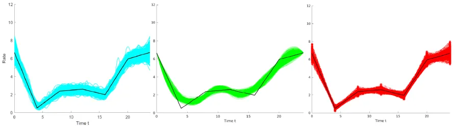
In Table 1 the averaged metrics from the three input modelling methods in the first experiment are presented. Recall that the true intensity in this case was piecewise-linear. In Table 1 the spline-based method is denoted ‘SPL’, the piecewise-quadratic method ‘PQ’ and the piecewise-linear method ‘PL’. In addition to Table 1, Figure 1 displays the output of theG=500 fits of the intensity function for the three methods form=30 days of arrival observations. The spline-based method is displayed on the left (cyan), the piecewise-quadratic representation in the centre (green), and the piecewise-linear representation is on the right (red). The plots also display the true piecewise-linear intensity (black).

Table 1: The average maximum absolute difference, ¯ζ, and the average integrated absolute difference, ¯δ, fromG=500 fits of the intensity function using three levels of input datam=15,30 and 100. The true intensity function,λc(t), in this experiment was piecewise-linear.

m=15 m=30 m=100

Method ζ¯ δ¯ ζ¯ δ¯ ζ¯ δ¯ SPL 0.978 6.288 0.805 4.879 0.548 3.076 PQ 5.441 8.177 5.383 7.452 5.356 6.844 PL 0.701 4.646 0.513 3.303 0.275 1.802

The piecewise-linear method performed the best in all three experiments, but this was to be expected given that the true intensity was piecewise-linear and the interval number and placements were known. The spline-based method also performs well; both averaged metrics are only slightly higher than those from the piecewise-linear representation for all three levels of input data. The piecewise-quadratic method performs the worst for all three levels of input data, m. In particular the average maximum absolute gap for this method is much higher than the other methods. In Figure 1 we can see what causes this behaviour, as the piecewise-quadratic function appears to smooth over the sharp corners of the truly piecewise-linear intensity function.

Another comment that should be made is that although both the piecewise-linear and piecewise-quadratic methods require knowledge of the number and location of the intervals on which their representations are built, this does not mean that the true interval locations were the best choice from which to build the piecewise-quadratic function in this experiment. The way the piecewise-quadratic function smooths over the corners of the truly piecewise-linear intensity in Figure 1 indicates that the method lacks the flexibility to represent those parts of the intensity. Additional flexibility could be gained within the MNO-PQRS method by using a larger number of intervals in the initial piecewise-constant function from which it is built.

In reality it is unlikely that the number and position of the intervals on which the piecewise representations are built are known, even if the function is truly piecewise-linear, which is also unlikely. In fact, unless the intensity is truly piecewise it is impossible to say what the correct placement of the intervals is. Our next experiment was therefore to compare the three methods when the true intensity function was a smooth function. In this experiment both the number and placement of the intervals required for the piecewise-linear and piecewise-quadratic methods for the best-possible fit were unknown. At this point a subjective number and placement of the intervals could have been used but we chose to utilise a data-driven method. Given

Table 2: The average maximum absolute difference, ¯ζ, and the average integrated absolute difference, ¯δ, fromG=500 fits of the intensity function using three levels of input datam=15,30 and 100. The true intensity function, λc(t), in this experiment was a smooth, cyclic sinusoidal function with an additional peak.

m=15 m=30 m=100

Method ζ¯ δ¯ ζ¯ δ¯ ζ¯ δ¯ SPL 0.892 7.754 0.674 5.738 0.450 3.575 PQ 4.175 8.814 4.073 6.518 4.011 3.758 PL 2.331 20.898 2.064 16.885 1.490 11.220

arrival-time observations the method presented by Chen and Schmeiser (2019) selects the optimal number of equal-length intervals from which to run the MNO-PQRS method. As before, in this experiment the intensity function was fitG=500 times for each method for the three levels of input data m=15,30 and 100. For each dataset the method of Chen and Schmeiser (2019) was used as a pre-processing tool to select the optimal number of intervals from which to build the piecewise-quadratic function. The number of intervals over the G=500 fits varied from 4 to 11 intervals for m=15 and 30 days of data and 4 to 18 intervals form=100. The number and positioning of intervals chosen for the MNO-PQRS method was also used for the piecewise-linear method in this experiment. An important point to make clear is that the placement and number of intervals used to build the piecewise-linear and piecewise-quadratic functions has a large effect on the resulting representation. The spline-based method, on the other hand, only requires that a large number of B-splines,n, are used, and the knots used to construct these are spaced uniformly throughout the interval.

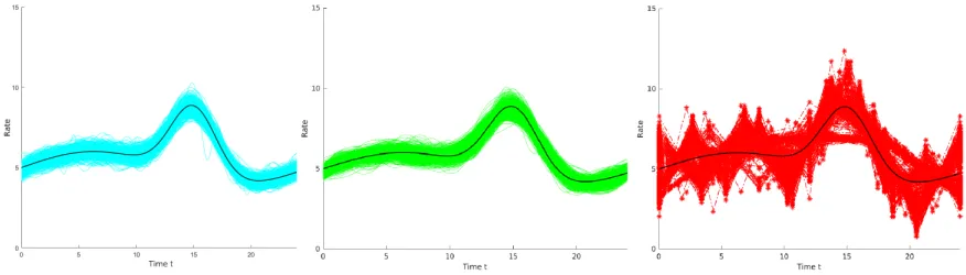
The smooth intensity function for which we compare the three methods is a cyclic function as seen in Figure 2 (black). This function was constructed from a sinusoidal function with an additional peak at time t=15. The averaged metrics from theG=500 replications are reported in Table 2. In addition to Table 2, Figure 2 displays the output of theG=500 fits of the intensity function for the three methods form=30 days of arrival observations.

It is clear from Table 2 that, for all three levels of input data, the spline-based method outperforms both the piecewise-quadratic and piecewise-linear methods in terms of the average maximum absolute gap and the average integrated absolute difference. In particular, the spline-based method seems to dominate the other methods by quite a margin when considering the average maximum absolute gap, ¯ζ. Note that, all methods are seen to improve as the number of observations of the whole interval,m, increases.

In this experiment the piecewise-linear method appears to perform particularly poorly in terms of the average integrated-absolute difference. This highlights the importance of knowing the number and placement of intervals for this method. In Figure 2,G=500 fits of the intensity givenm=30 observations of the arrival process are presented. From Figure 2 the spline-based method, and the piecewise-quadratic method can be seen to give reasonable representations; in almost all G=500 replications both methods appear to follow the shape of the true intensity well. The piecewise-linear method on the other hand appears to be more erratic, and in a reasonably large number of cases smooths over the peak in the true intensity function. Looking in more detail at the results from Figure 2 we found that, for all G=500 fits of the intensity function, the integrated absolute difference,δ, was larger for the piecewise-linear representation than the other methods. There was also no noticeable relationship between the number of intervals and recording a high integrated absolute difference for the piecewise-linear method.

In summary, in our second experiment the spline-based method was shown to dominate its competitors in terms of the metrics of average maximum absolute difference and average integrated absolute difference. These metrics are measures of how well a method recovers the underlying intensity function of a NHPP. If a simulation experiment were to be performed with an arrival process described by the smooth intensity function used in this experiment, it is our belief that the spline-based method would on average pass the least input modelling error to the output of a simulation model as it appears to recover the underlying true arrival rate better than its competitors.

5.2 Realistic Example

We now present a realistic example for fitting the spline-based model to arrivals from an A&E department. The arrival rate to the A&E system was believed to follow a cyclic pattern over a week-long period. In this experiment we focused on observations over the summer months: June, July and August, from the years 2011/12 as we believed the weekly arrival behaviour in this period to be similar. Summer is also a season with few public holidays which are believed to cause fluctuations to arrivals to A&E. In total there were m=24 weeks of observations from the A&E department.

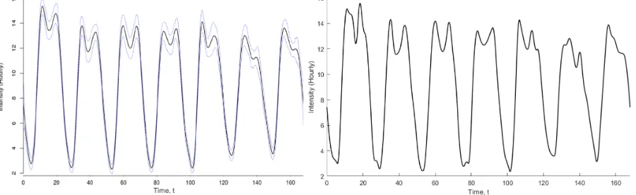
Before fitting the spline function we considered the assumption that the arrivals follow a NHPP. Using a chi-square goodness-of-fit test we checked whether the total number of arrivals on each day of the week can be said to be Poisson. In conclusion we had significant evidence to reject that the arrival counts on Wednesdays, Thursdays and Fridays were Poisson; the counts on these days were particularly overdispersed in comparison to a Poisson distribution. Despite this, in reality, NHPPs are often used as input models without checking such assumptions. We will therefore proceed to fit the arrival data using our spline-based method but we will also fit the arrival rate using the MNO-PQRS method as it has no dependency on the input process being Poisson. The spline fit, constructed from 56 uniformly spaced knot points i.e. n=52 B-splines, can be seen on the left of Figure 3 along with a 95% pointwise confidence interval.

The choice of 56 knots corresponds to a knot every 3 hours with knots at the same time each day; note that, although placement of the knots at the same time is not necessary, it seemed natural in this cyclic context. The MNO-PQRS fit can be seen on the right of Figure 3. Note that prior to running MNO-PQRS the pre-processing method of Chen and Schmeiser (2018) was used and split the week into 88 intervals of equal length.

The resulting representations in Figure 3 exhibit very similar behaviour. On Thursday and Friday, the 4thand 5thcycles in the arrival rate, where the p-value of the goodness-of-fit test was particularly significant (<1×10−6) we appear to see the most discrepancy between the fits but even there the difference is not great. Of course, since this is real-world example we do not know the true underlying arrival rate, and therefore which method is closer to the truth, but the similarity between the representations indicates that the spline-based method is not greatly sensitive to data which diverges from Poisson assumptions in terms of being overdispersed.

6 CONCLUSION

In this paper we presented a new spline-based input modelling method. This method utilises the penalised log-likelihood for fitting the intensity function of a NHPP given arrival-time observations. We also presented a simple method for generating arrivals from the fitted spline-based representation. This method took advantage of the composition of the spline function as a linear combination of B-spline basis functions with known maximums. An algorithm was also presented to assist arrival generation in practice.

Compared to two recent methods in the literature, the spline-based method was seen to perform best in terms of the average integrated absolute difference and average maximum absolute gap when the true intensity function was smooth. The chosen metrics were indicators of how well the true arrival rate function was recovered. When the true intensity was piecewise-linear the spline-based input modelling method was also seen to perform well. Both experiments highlighted the advantage of not requiring prior knowledge of the number and placement of intervals for the spline-based method.

A realistic input modelling situation, given observations from an A&E department, was also presented. We showed that, even when the observations departed from Poisson assumptions, the spline-based technique returned a similar rate function to the one produced by MNO-PQRS, which was designed to fit the rate functions of general input processes. This suggests that the spline-based method is not sensitive to overdispersed observations.

In practice, arrival counts are sometimes recorded instead of arrival-times. Our method could be extended to work for arrival count data through a simple modification of the log-likelihood. In the same way, provided an appropriate likelihood can be derived, the penalised log-likelihood method could be extended for use with other non-stationary non-Poisson arrival processes. We leave these extensions for future work.

Another area of interest for future work is how to choose a suitably large number of B-splines, n, from which to build the spline function. Too few basis functions will lead to a lack of flexibility of the spline-based model and thus no penalisation, but too many can lead to a discrepancy between the second-order approximation used in the trust region algorithm and the objective function. The number of basis functions chosen should be large enough to ensure that the true intensity function can reasonably approximated by a cubic over each interval. Choosingn“large enough” is therefore a question of interest. ACKNOWLEDGEMENTS

REFERENCES

Cavanaugh, J. E., and A. A. Neath. 2011. “Akaike’s Information Criterion: Background, Derivation, Properties, and Refinements”. InInternational Encyclopedia of Statistical Science, 26–29. Springer. Channouf, N. 2008.Mod´elisation et Optimisation d’un Centre d’appels T´el´ephoniques: ´etude du Processus

d’arriv´ee. Ph. D. thesis, D´epartement d’Informatique et de Recherche Op´erationnelle, Universit´e de Montr´eal, Montr´eal.

Chen, H., and B. Schmeiser. 2015. “I-SMOOTH: Iteratively Smoothing Mean-Constrained and Nonnegative Piecewise-Constant Functions”.INFORMS Journal on Computing 25(3):432–445.

Chen, H., and B. W. Schmeiser. 2017. “MNO–PQRS: Max Nonnegativity Ordering Piecewise-Quadratic Rate Smoothing”. ACM Transactions on Modeling and Computer Simulation27(3):1–19.

Chen, H., and B. W. Schmeiser. 2018. “MISE-Optimal Grouping of Point-Process Data with a Constant Dispersion Ratio”. In Proceedings of the 2018 Winter Simulation Conference, edited by M. Rabe, A. A. Juan, N. Mustafee, A. Skoogh, S. Jain, and B. Johansson, 1563–1574. Piscataway, New Jersey: Institute of Electrical and Electronics Engineers, Inc.

Chen, H., and B. W. Schmeiser. 2019. “MISE-Optimal Grouping for MNOPQRS Rate-Function Estimators”. Technical report, Chung Yuan Christian University, Taiwan.

Conn, A. R., N. I. Gould, and P. L. Toint. 2000. Trust Region Methods, Volume 1. Philadelphia: Society for Industrial and Applied Mathematics (SIAM).

de Boor, C. 1978.A Practical Guide to Splines, Volume 27. New York: Springer-Verlag.

Dixon, M. and T. Ward 2018. “Takeuchi’s Information Criteria as a Form of Regularization”. https: //arxiv.org/pdf/1803.04947.pdf.

Green, L. 2006. “Queueing Analysis in Healthcare”. In Patient Flow: Reducing Delay in Healthcare Delivery, edited by R. W. Hall, 281–307. Boston: Springer.

Kao, E. P., and S.-L. Chang. 1988. “Modeling Time-Dependent Arrivals to Service Systems: A Case in using a Piecewise-Polynomial Rate Function in a Nonhomogeneous Poisson Process”. Management Science34(11):1367–1379.

Kim, S.-H., and W. Whitt. 2014. “Are Call Center and Hospital Arrivals Well Modeled by Nonhomogeneous Poisson Processes?”. Manufacturing & Service Operations Management 16(3):464–480.

Klein, R. W., and S. D. Roberts. 1984. “A Time-Varying Poisson Arrival Process Generator”. Simula-tion 43(4):193–195.

Kuhl, M. E., J. R. Wilson, and M. A. Johnson. 1997. “Estimating and Simulating Poisson Processes Having Trends or Multiple Periodicities”. IIE Transactions29(3):201–211.

Kullback, S. 1997. Information Theory and Statistics. Courier Corporation.

Lam, H. 2016. “Advanced Tutorial: Input Uncertainty and Robust Analysis in Stochastic Simulation”. In Proceedings of the 2016 Winter Simulation Conference, edited by T. M. K. Roeder, P. I. Frazier, R. Szechtman, E. Zhou, T. Huschka, and S. E. Chick, 178–192. Piscataway, New Jersey: Institute of Electrical and Electronics Engineers, Inc.

Lee, S., J. R. Wilson, and M. M. Crawford. 1991. “Modeling and Simulation of a Nonhomogeneous Poisson Process having Cyclic Behavior”. Communications in Statistics-Simulation and Computation 20(2-3):777–809.

Leemis, L. M. 1991. “Nonparametric Estimation of the Cumulative Intensity Function for a Nonhomogeneous Poisson Process”.Management Science37(7):886–900.

Lewis, P. A., and G. S. Shedler. 1976. “Statistical Analysis of Non-stationary Series of Events in a Data Base System”. Technical report, Naval Postgraduate School. Monterey, California.

Morgan, L. E., B. L. Nelson, A. C. Titman, and D. J. Worthington. 2019. “Detecting Bias due to Input Modelling in Computer Simulation”.European Journal of Operational Research. doi:https://doi.org/ 10.1016/j.ejor.2019.06.003.

of the 2016 Winter Simulation Conference, edited by T. M. K. Roeder, P. I. Frazier, R. Szechtman, E. Zhou, T. Huschka, and S. E. Chick, 370–381. Piscataway, New Jersey: Institute of Electrical and Electronics Engineers, Inc.

Nicol, D. M., and L. M. Leemis. 2014. “A Continuous Piecewise-Linear NHPP Intensity Function Estimator”. InProceedings of the 2014 Winter Simulation Conference, edited by A. Tolk, S. Y. Diallo, I. O. Ryzhov, L. Yilmaz, S. Buckley, and J. A. Miller, 498–509. Piscataway, New Jersey: Institute of Electrical and Electronics Engineers, Inc.

Pritsker, A., D. Martin, J. Reust, M. Wagner, J. Wilson, M. Kuhl, J. Roberts, O. Daily, A. Harper, E. Edwards, L. Bennett, J. Burdick, and M. Allen. 1996. “Organ Transplantation Modeling and Analysis”. InProceedings of the 1996 Western Multiconference: Simulation in the Medical Sciences, edited by A. J.G. and M. Katzper, 29–35. The Society for Computer Simulation, San Diego, California. R Core Team. 2018. R: A Language and Environment for Statistical Computing. Vienna, Austria: R

Foundation for Statistical Computing.

Reinsch, C. H. 1967. “Smoothing by spline functions”.Numerische mathematik10(3):177–183.

Shibata, R. 1989. “Statistical Aspects of Model Selection”. In From Data to Model, 215–240. Berlin, Heidelberg: Springer.

Song, E., B. L. Nelson, and C. D. Pegden. 2014. “Advanced Tutorial: Input Uncertainty Quantification”. In Proceedings of the 2014 Winter Simulation Conference, edited by A. Tolk, S. Y. Diallo, I. O. Ryzhov, L. Yilmaz, S. Buckley, and J. A. Miller, 162–176. Piscataway, New Jersey: Institute of Electrical and Electronics Engineers, Inc.

Viswanadham, N., and Y. Narahari. 1992. Performance Modeling of Automated Manufacturing Systems. Englewood Cliffs, New Jersey, Prentice Hall.

Zheng, Z., and P. W. Glynn. 2017. “Fitting Continuous Piecewise Linear Poisson Intensities via Maximum Likelihood and Least Squares”. In Proceedings of the 2017 Winter Simulation Conference, edited by W. K. V. Chan, A. D’Ambrogio, G. Zacharewicz, N. Mustafee, G. Wainer, and E. Page, 1740–1749. Piscataway, New Jersey: Institute of Electrical and Electronics Engineers, Inc.

AUTHOR BIOGRAPHIES

LUCY E. MORGANis a Development Lecturer in Simulation and Stochastic Modelling in the Department of Management Science at Lancaster University. Her research interests are input uncertainty in simulation models and arrival process modelling. Her e-mail address is [email protected].

BARRY L. NELSONis the Walter P. Murphy Professor in the Department of Industrial Engineering and Management Sciences at Northwestern University and a Distinguished Visiting Scholar in the Lancaster University Management School. He is a Fellow of INFORMS and IISE. His research centers on the design and analysis of computer simulation experiments on models of stochastic systems. His e-mail address is

[email protected].

ANDREW C. TITMANreceived his Ph.D. from the University of Cambridge and currently is Lecturer in Statistics in the Department of Mathematics and Statistics at Lancaster University. His research interests include survival and event history analysis and latent variable modelling, with applications in biostatistics and health economics. His e-mail address [email protected].