1
Innovation across cities
Kwok Tong Soo*
Lancaster University
May 2017
Abstract
This paper examines the distribution of patenting activity across cities in the OECD,
using a sample of 218 cities from 2000 to 2008. We obtain three main results. First,
patenting activity is more concentrated than population and GDP. Second, patenting
activity is less persistent than population and GDP, especially in the middle of the
distribution. Third, in a parametric model, patenting does not exhibit
mean-reversion, and is positively associated with GDP and population density. Our results
suggest that policymakers can influence the amount of innovative activity through
the use of appropriate policies.
JEL Classification: R1, O3.
Keywords: Patents; Zipf’s Law; transition probability; dynamic panel data; local
linear estimator.
* Department of Economics, Lancaster University Management School, Lancaster LA1 4YX, United Kingdom.
Tel: +44(0)1524 594418. Email: [email protected]
1
“The mysteries of the trade become no mysteries; but are as it were in the air…”
Alfred Marshall (1920), Principles of Economics, 8th Edition, p.225.
1.
INTRODUCTION
Since at least Marshall (1920) it has been argued that forces of agglomeration may lead to the
formation of industrial clusters, and by extension, cities. As has been discussed in greater detail
elsewhere (Krugman, 1991, Fujita et al, 1999), Marshall identified three reasons for the spatial
concentration of economic activity: knowledge spillovers, thick markets for specialised skills,
and the backward and forward linkages associated with large local markets. Because of the
presence of knowledge spillovers, cities are not only the centre of economic activity, but also
the focal point of innovative activity. Indeed, if it is argued that innovative activity makes use
of all three of Marshall’s external economies, then innovative activity should be even more
concentrated than economic activity in general. Anecdotal evidence supports this idea; for
instance, in 2008 Tokyo had 27 percent of Japan’s population, but 32.3 percent of GDP, and
34.3 percent of the number of patents.
This paper explores the distribution of patenting activities across cities, the persistence and
growth of patenting in cities, and the determinants of patenting activity. In so doing, we make
use of methods developed for the analysis of city populations, and city population thus acts as
a useful benchmark to compare with patents. We use a sample of 218 cities from OECD
countries, from 2000 to 2008, and obtain three main results. First, patenting is more unevenly
distributed across cities than population or GDP. Second, patenting is less persistent than both
population and GDP, especially in the middle of the distribution. Third, even after controlling
2
associated with GDP and population density. Taken together our results suggest that it may be
possible for policymakers to implement policies that encourage innovation in cities.
Usually in this literature the analysis is performed using a sample of cities within a country.
One reason for this is that different countries may have different institutional settings, which
may influence the distribution of innovative activity in the country. Our use of data for cities
across OECD countries may be defended along the following lines. First, we focus on
innovations, and innovators are often highly skilled, footloose people, who may be more likely
to move across international borders. In this context, the cities in the sample are the largest
cities in each country with a minimum population of 500,000, so may be viewed as substitutes
(even if imperfect) by innovators. Second, some of the theoretical literature on city systems
(for instance, Gabaix, 1999) shows that, if each region or country follows Zipf’s Law (which
in turn arises from Gibrat’s Law), then the overall distribution will follow Zipf’s Law as well.
Hence, using a larger geographic region as the sample should not materially influence the
analysis. Indeed, we are unable to reject the null hypothesis that Gibrat’s Law of proportional
growth holds for patents, thus suggesting that the mechanism identified by Gabaix (1999) may
apply in our sample. Third, in estimating the determinants of innovative activity, we make use
of methods which control for unobserved city-specific effects, so institutional frameworks
which are different across countries should not influence the results.
This paper is related to three strands of literature. First, the literature on the production of
knowledge in cities is discussed in Audretsch and Feldman (1996, 1999) and has been surveyed
in Audretsch and Feldman (2004). This line of research is mainly focussed on the impact of
industrial concentration and diversity on the productivity of R&D (“spillovers”). A closely
3
composition on economic growth in cities. Unlike this literature, our focus is not on R&D
spillovers, but rather on the distribution of innovation across cities, and the factors that may
explain the distribution.
There is an associated branch of the literature which examines innovative and creative activities
in cities. This includes OhUallachain (1999), Berry and Glaeser (2005), Bettencourt et al (2007,
2010), and Strumsky and Thill (2013). However, much of this literature focuses on US cities,
and is primarily interested in describing the distribution of innovative activity across cities. In
the present paper, we use an international dataset comprising the largest cities in the OECD,
thus allowing us to see whether any trends that we observe operate across national boundaries.
In addition, whilst we are also interested in how innovative activity is distributed across cities,
we extend the analysis to consider the persistence and evolution of innovative activity over
time.
Methodologically, since the paper presents evidence on the distribution and growth of
innovation in cities, it is related to the literature on the size distribution and growth of cities, as
discussed in Gabaix and Ioannides (2004), Eaton and Eckstein (1997), Black and Henderson
(2003), Dobkins and Ioannides (1999, 2001), Ioannides and Overman (2001, 2003, 2004), Soo
(2005, 2007), and Bosker et al (2008). On the distribution of innovation in cities, we make use
of the concept of Zipf’s Law (Zipf, 1949), that the size of cities follows a Pareto distribution.
Gabaix and Ibragimov (2011) develop a simple way of improving the performance of OLS
estimates of Zipf’s Law. On the persistence of innovation in cities, we make use of the concept
of transition probability matrices. Finally, on the growth of innovation over time, we make use
of both parametric and non-parametric approaches to describe the growth patterns of
4
The next section discusses the data used in this paper. This is followed in Section 3 by the
analysis of the distribution of innovative activity, in Section 4 by the persistence of innovative
activity, in Section 5 by the growth of innovative activity, and in Section 6 by the determinants
of innovative activity. Because of the wide range of methods used, they will be discussed within
each section to maximise clarity. The final section concludes.
2.
DATA
The data is obtained from the OECD Metropolitan Database, which contains data for metro
areas with a population of 500,000 or more across OECD countries. Metro areas are defined
following a harmonised functional definition developed by the OECD in OECD (2012). This
is important, since studies using data across countries can be affected by the fact that the data
may not be defined consistently across countries. We avoid this by using data from the OECD
Metropolitan Database. There are a total of 275 cities from 28 OECD countries. Patent data is
available for 218 metro areas from 16 countries from 2000 to 2008, and represents a count of
the number of patent applications by the city of the inventor1. The dataset also includes other
variables, such as population, geographical and administrative information, labour markets,
and GDP (measured in US$ in constant prices and constant PPPs with a base year of 2005).
< Place Table 1 here >
< Place Table 2 here >
Table 1 shows the distribution of cities across countries in the data. Most major OECD
5
United Kingdom, for which patent data are not available. Table 2 reports the correlation
between patenting activity, economic activity as measured by GDP, and population in our
sample, for 2008. There is high correlation between all three variables; large cities are also
cities with lots of economic activity, and lots of innovative activity. Figure 1 graphically
represents the same information as in Table 22.
< Place Figure 1 here >
< Place Table 3 here >
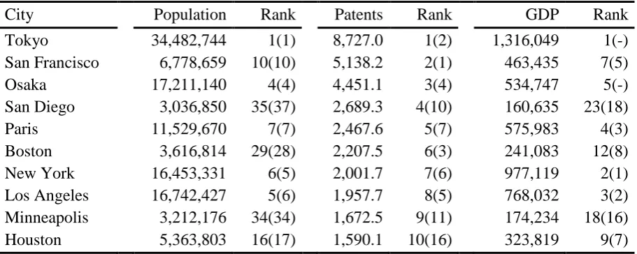
Table 3 presents the ten cities with the largest number of patents in 2008, along with their
population and GDP, with their 2000 ranks in parentheses. Although in general the cities with
the most patents also have the most population and the highest GDP, there are some anomalies.
For instance, San Francisco is associated with Silicon Valley, and has a larger number of
patents than would be predicted by its population or GDP. Similarly, Boston is associated with
biotechnology and the IT cluster of Route 128, while San Diego is a centre for biotechnology
and communications technology. Two other features of Table 3 are noteworthy. First,
comparing rankings between 2008 and 2000 shows that populations are persistent over time,
whereas GDP and patents are less so; we shall return to this in Section 4 below. Second, cities
in the United States dominate the table, occupying seven of the top ten patenting cities in 2008;
the equivalent number in 2000 was five of the top ten from the United States. This emphasises
the United States’ dominance in innovation, although it may be partially driven by cities in
countries which have been omitted from our sample due to lack of data, for instance London
6
3.
THE DISTRIBUTION OF INNOVATIVE ACTIVITY
In this section we compare the distribution of patents across cities with the distribution of
population and economic activity. If the idea behind Marshall’s external economies is correct,
then we would expect that patents are going to be more highly concentrated than economic
activity in general, and that economic activity is in turn going to be more highly concentrated
than population.
< Place Table 4 here >
A simple way to compare the distribution of the three variables is to compare the standard
deviations of the natural logs of the variables. This is reported in Table 4, where it is clear that
population has the smallest standard deviation, followed by GDP and patents. That is, as
predicted by Marshall’s theory, patents are more concentrated in a small number of cities than
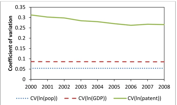
economic activity and population. Figure 2 plots the coefficient of variation (standard deviation
divided by the mean) over time for the three variables. Not only does Figure 2 show the same
patterns as in Table 4, in addition it shows that the coefficient of variation of patenting is
decreasing over time, unlike for population and GDP, which have remained fairly constant over
the time period of Figure 2. This suggests that patents are becoming less concentrated over
time. Figure 3 plots the kernel density functions for the three variables in 2008 (in natural logs),
using an Epanechnikov kernel and the Silverman (1986) rule of thumb bandwidth. This figure
again shows the greater dispersion of patents compared to the other two variables, which
indicates greater concentration of patents in the cities which undertake the most patenting.
7 < Place Figure 3 here >
An alternative way of comparing the distribution of these variables, which has been popular in
the city size literature, is to use Zipf’s Law, which states that the size distribution follows a
simple Pareto distribution with shape parameter equal to 1. To operationalise this idea, let:
𝑅𝑅 =𝐴𝐴𝑆𝑆−𝛼𝛼, (1)
where 𝑅𝑅 is the rank of a city in terms of its size (with the largest city being ranked 1), 𝑆𝑆 is the
size of the city used in constructing 𝑅𝑅, and 𝐴𝐴 and 𝛼𝛼 are parameters. Taking natural logs of
equation (1) and adding a random error term 𝜖𝜖 gives:
ln𝑅𝑅 = ln𝐴𝐴 − 𝛼𝛼ln𝑆𝑆+𝜖𝜖. (2)
Thus the Zipf’s Law prediction is that there is a linear relationship between the natural log of
the rank and the natural log of the size. The parameter 𝛼𝛼 is a measure of the inequality of the
distribution; the larger is 𝛼𝛼, the more equal is the distribution across cities.
< Place Figure 4 here >
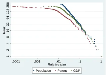
Figure 4 plots the scatter diagram of the rank of a city versus its size as measured by population,
GDP and number of patents, for 2008, on a log scale with the largest value normalised to 1.
The figure shows that, whilst there appears to be a roughly linear relationship between log of
rank and log of population, there is pronounced curvature for GDP and especially for patents.
Another observation that can be made from Figure 4 is that, overall, population is more equally
distributed than GDP, which in turn is more equally distributed than patents. If Marshall’s
external economies argument is correct, then this is what we would expect; that larger cities
8
proximity to other innovating agents will yield greater external economies than other types of
economic activity.
Gabaix and Ioannides (2004) show that OLS estimation of equation (2) leads to biased results,
while Gabaix and Ibragimov (2011) show that a simple way to improve OLS estimation of
equation (2) is instead to estimate the following equation:
ln�𝑅𝑅 −12�= ln𝐴𝐴 − 𝛼𝛼ln𝑆𝑆+𝜖𝜖, (3)
with the standard error of 𝛼𝛼 being given by (2⁄𝑛𝑛)1 2⁄ 𝛼𝛼, where 𝑛𝑛 is the number of cities. The
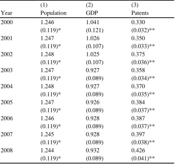
results of estimating equation (3) for each year for population, GDP and patents are presented
in Table 5, which reports the values of 𝛼𝛼. Comparing across the three variables, the coefficients
for population are always larger than for GDP, which in turn are always larger than for patents.
This confirms the visual inspection of Figure 4 discussed above; population is the most equally
distributed across cities, followed by GDP, with patents being the most unequally distributed.
< Place Table 5 here >
Comparing the coefficients across time, the coefficient for population is almost constant over
time. The coefficient for GDP shows greater variation over time (although part of the variation
is driven by data availability), while the coefficient for patents shows the greatest variation
over time. Especially for patents, there appears to be a trend of rising coefficients, which
indicates that patenting activity is becoming more dispersed over time. This may indicate that
the Marshallian external economies in innovative activity are becoming weaker over time,
perhaps in response to developments in communication technology, and supports the analysis
using the coefficient of variation in Figure 2. In terms of Zipf’s Law (the hypothesis that 𝛼𝛼 =
9
populations are more equal in size than would be predicted by Zipf’s Law, whereas patents are
less equally distributed than the Zipf’s Law prediction3.
4.
THE PERSISTENCE OF INNOVATIVE ACTIVITY
In this section we examine how persistent is innovative activity, relative to population and
GDP. We make use of transition probability matrices first introduced into the economic growth
literature by Quah (1993), and used in the city population literature by Eaton and Eckstein
(1997), Dobkins and Ioannides (2000), and Black and Henderson (2003). We group the sample
of cities into ten cells in each year. Let 𝐹𝐹𝑡𝑡 be a 10 × 1 vector which denotes the distribution of
sizes across cities at time 𝑡𝑡. Assume that 𝐹𝐹𝑡𝑡 evolves according to:
𝐹𝐹𝑡𝑡+1= 𝑀𝑀𝐹𝐹𝑡𝑡, (4)
where 𝑀𝑀 is a 10 × 10 transition probability matrix, mapping the assignment from period 𝑡𝑡 into
an assignment in period 𝑡𝑡+ 1. Following Dobkins and Ioannides (2000), we define the vector
𝐹𝐹𝑡𝑡 based on the deciles of the distribution4. Since we have data from 2000 to 2008, and since
population changes only slowly, we present results for the 8-year transition matrix between
2000 and 20085.
< Place Table 6 here >
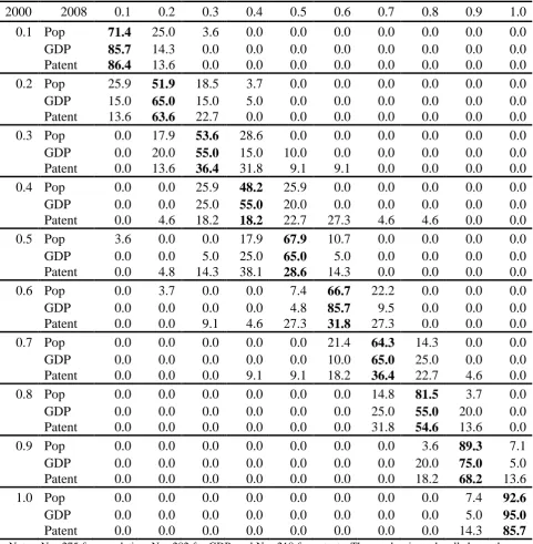
Table 6 presents the results, arranged so as to make the comparison between the three variables
(population, GDP and patents) as clear as possible. Overall, patents exhibit less persistence
than population and GDP; the diagonal elements of the matrix (in bold type) are, on average,
smaller for patents than for population and GDP. This is especially true in the middle of the
10
persistent they are over time6. Indeed, the mobility of a city both up and down the distribution
of patents is quite large; a city which in the year 2000 was between the 60th and 70th percentiles
of the distribution of patents, could by the year 2008 lie anywhere between the 30th and 90th
percentiles.
Nevertheless, where patenting activity does exhibit considerable persistence, is at both ends of
the distribution. Cities in the bottom 10th percentile of the distribution of patents in the year
2000 only had a 13.6 percent chance of moving up to the 20th percentile by 2008, which is a
lower likelihood of transition than for both population and GDP. A similar though less
pronounced pattern can be observed at the top of the distribution. What this suggests is that
cities that start off with low levels of patenting activity, struggle to develop any innovation
capacity (or perhaps choose to specialise in non-innovation-intensive activities); cities with lots
of patenting activity benefit from Marshallian external economies, while cities in between may
end up in either a virtuous or a vicious cycle of innovation.
5.
THE GROWTH OF INNOVATIVE ACTIVITY
In this section we make use of both parametric and nonparametric approaches to examine the
growth of innovative activity. Perhaps a natural starting point is to assume that city growth and
city size are independently distributed; that is, that city growth obeys Gibrat’s Law. We follow
Black and Henderson (2003) in estimating the following equation:
ln(𝑆𝑆𝑖𝑖𝑡𝑡)−ln(𝑆𝑆𝑖𝑖𝑡𝑡−1) =𝛽𝛽𝑖𝑖+𝛿𝛿𝑡𝑡+𝛾𝛾ln(𝑆𝑆𝑖𝑖𝑡𝑡−1) +𝜖𝜖𝑖𝑖𝑡𝑡, (5)
where 𝛽𝛽𝑖𝑖 are city fixed effects and 𝛿𝛿𝑡𝑡 are time fixed effects. Hence, both here and in Section 6,
11
variables (and therefore any city- or country-specific effects such as different institutional
arrangements, are partialled-out). Equation (5)7 may be rewritten as follows:
ln(𝑆𝑆𝑖𝑖𝑡𝑡) =𝛽𝛽𝑖𝑖 +𝛿𝛿𝑡𝑡+ (1 +𝛾𝛾) ln(𝑆𝑆𝑖𝑖𝑡𝑡−1) +𝜖𝜖𝑖𝑖𝑡𝑡. (6)
The null hypothesis implied by Gibrat’s Law is that 𝛾𝛾 = 0 or 1 +𝛾𝛾 = 1. Given the null
hypothesis of Gibrat’s Law, the error term cannot be serially correlated, so we use a
conventional fixed-effects model to estimate equation (6). Here, unlike in the previous section,
we make use of data on an annual basis.
< Place Table 7 here >
The estimated values of 1 +𝛾𝛾 for population, GDP and patents using the conventional
fixed-effects model are reported in columns (1) to (3) of Table 7. Standard errors are clustered by
city to allow for heteroskedasticity and within-city correlation in the residuals, and all results
reported include both year and city fixed effects. For all three variables of interest, the Gibrat’s
Law null hypothesis that 1 +𝛾𝛾= 1 is rejected in favour of the alternative that 1 +𝛾𝛾 < 1. That
is, rather than random growth, we find evidence of mean-reversion; large cities grow more
slowly than small ones. The coefficient is smallest (hence mean reversion is the quickest) for
patents, followed by GDP and population. Similarly to the results of the previous section,
patents exhibit less persistence than GDP and especially population.
However, parametric models such as equation (6) do not give a complete picture of the
relationship between size and growth of cities. Therefore, we supplement equation (6) with a
non-parametric estimator. Consider the following general model of the relationship between
the size and growth of a city8:
12
where Δ𝑆𝑆𝑖𝑖𝑡𝑡 =𝑆𝑆𝑖𝑖𝑡𝑡+1− 𝑆𝑆𝑖𝑖𝑡𝑡. However, the functional form 𝑚𝑚(∙) is not specified. 𝑚𝑚(∙) may be
estimated using a local weighted average estimator:
𝑚𝑚�(𝑆𝑆0) =∑𝑁𝑁𝑖𝑖=1𝑤𝑤𝑖𝑖0,ℎΔ𝑆𝑆𝑖𝑖𝑡𝑡, (8)
where the weights 𝑤𝑤𝑖𝑖0,ℎ = 𝑤𝑤(𝑆𝑆𝑖𝑖𝑡𝑡,𝑆𝑆0,ℎ) sum to 1. The weights increase as 𝑆𝑆𝑖𝑖𝑡𝑡 becomes closer
to 𝑆𝑆0. The Nadaraya-Watson or kernel regression estimator (used for instance in the cities
literature by Ioannides and Overman, 2003 and Eeckhout, 2004) uses a kernel weighting
function 𝐾𝐾(∙), so that:
𝑚𝑚�(𝑆𝑆0) =
1
𝑁𝑁ℎ∑𝑁𝑁𝑖𝑖=1𝐾𝐾�𝑆𝑆𝑖𝑖𝑖𝑖−𝑆𝑆0ℎ �Δ𝑆𝑆𝑖𝑖𝑖𝑖 1
𝑁𝑁ℎ∑𝑁𝑁𝑖𝑖=1𝐾𝐾�𝑆𝑆𝑖𝑖𝑖𝑖−𝑆𝑆0ℎ �
. (9)
The constant ℎ is the bandwidth of the kernel function. The kernel regression estimator can be
obtained by minimising ∑ 𝐾𝐾 �𝑆𝑆𝑖𝑖𝑖𝑖−𝑆𝑆0
ℎ �(Δ𝑆𝑆𝑖𝑖𝑡𝑡− 𝑚𝑚0)2 𝑁𝑁
𝑖𝑖=1 with respect to 𝑚𝑚0. That is, the kernel
regression estimator is a local constant estimator, because it assumes that 𝑚𝑚(𝑆𝑆) is a constant in
the local neighbourhood of 𝑆𝑆0. Instead, one can let 𝑚𝑚(𝑆𝑆) be linear in the neighbourhood of 𝑆𝑆0,
so that 𝑚𝑚(𝑆𝑆) =𝑎𝑎0 +𝑏𝑏0(𝑆𝑆 − 𝑆𝑆0) in the neighbourhood of 𝑥𝑥0. The local linear estimator
minimises:
∑ 𝐾𝐾 �𝑆𝑆𝑖𝑖𝑖𝑖−𝑆𝑆0
ℎ � �Δ𝑆𝑆𝑖𝑖𝑡𝑡− 𝑎𝑎0− 𝑏𝑏0(𝑆𝑆𝑖𝑖𝑡𝑡− 𝑆𝑆0)� 2 𝑁𝑁
𝑖𝑖=1 (10)
with respect to 𝑎𝑎0 and 𝑏𝑏0, where 𝐾𝐾(∙) is a kernel weighting function. Then 𝑚𝑚�(𝑆𝑆) =𝑎𝑎�0+
𝑏𝑏�0(𝑆𝑆 − 𝑆𝑆0) in the neighbourhood of 𝑆𝑆0. Fan (1992) and Fan and Gijbels (1996) argue that the
local linear estimator has many attractive properties. The local linear estimator is the best
among all linear smoothers, and has a smaller bias than the Nadaraya-Watson estimator,
especially at the boundaries of the support of 𝑆𝑆𝑖𝑖𝑡𝑡. Compared to other local regression estimators
such as LOWESS (Cleveland, 1979), the local linear estimator is much less computationally
intensive. On the other hand, Hansen (2017) argues that the Nadaraya-Watson estimator
outperforms the local linear estimator when 𝑚𝑚(𝑆𝑆) is close to a flat line, but the opposite is true
13
In implementing a nonparametric estimator of the type just described, there are three
considerations9. The first consideration is the degree of polynomial used. Although the local
constant and local linear estimators have been described above, these can be extended to local
polynomial estimators. However, high-order local polynomial estimators may face the curse of
dimensionality; that is, data sparsity becomes more of a problem for higher order polynomials.
This increases the variance of the estimate. We therefore use the local linear estimator for its
superior performance relative to the Nadaraya-Watson estimator, but also to keep the order of
the polynomial low to reduce the curse of dimensionality. A second consideration is the kernel
weighting function used; possible choices include the Gaussian, Epanechnikov, uniform,
biweight and triweight kernels. The Epanechnikov kernel has the smallest integrated mean
squared error (IMSE; see Wand and Jones, 1995), so we use this kernel. However, the
difference between the Epanechnikov kernel and other kernels is often small.
A third consideration is the bandwidth ℎ used. Larger values of ℎ will reduce the variance,
since more points will be included in the estimate. However, as ℎ increases, the average
distance between the local points ans 𝑆𝑆0 will also increase, which can result in a larger bias and
oversmoothing. We use the rule-of-thumb plugin estimator of the asymptotically optimal
constant bandwidth (note this is not the same as Silverman’s (1986) rule of thumb bandwidth
estimator). A confidence interval is also reported for the local linear estimator. The residual
variance at each smoothing point is estimated by locally fitting a polynomial of order 3, and
the bandwidth used for the confidence interval is 1.5 ×ℎ. To implement this estimator, we
standardise the size and growth of cities by subtracting the annual mean from the raw data and
14 < Place Figure 5 here >
Figure 5 reports the results of the nonparametric estimates, for the three variables population,
GDP and patents, together with a 95 percent confidence interval; the scatterplot of data points
has been omitted for clarity. From this figure it can be seen that GDP most closely follows the
Gibrat’s Law null hypothesis of no relationship between GDP and GDP growth. Even here
there is some evidence that cities with larger GDP exhibit slower growth than cities with
smaller GDP. For population, cities in the middle of the population distribution grow faster
than those at both ends of the distribution. For patents, the confidence bands are much narrower
than for the other two variables, and, consistently with the parametric results in Table 7, it is
cities with the fewest patents that experience the fastest patent growth rates. However, cities
between 1 and 2 standard deviations below the mean experience slower patent growth rates on
average. Without additional analysis it is difficult to interpret this finding. However, the result
bears some similarity with those obtained by Davis and Weinstein (2008), hence may indicate
the presence of mean-reversion or multiple equilibria. Whilst it may be relatively easy for cities
with few patents to rapidly increase their patenting rate, it may be more difficult to step up to
the next level and join the ranks of the major innovating centres.
6.
THE DETERMINANTS OF INNOVATIVE ACTIVITY
In the previous section, one general conclusion that emerged was that cities with relatively
fewer patents, experience more rapid growth in patenting activity. In this section we explore
this further, and investigate the possible determinants of innovative activity in a city. Similarly
to Black and Henderson (2003), we extend equation (6) in the previous section to include
15
ln(𝑆𝑆𝑖𝑖𝑡𝑡) =𝛽𝛽𝑖𝑖 +𝛿𝛿𝑡𝑡+ (1 +𝛾𝛾) ln(𝑆𝑆𝑖𝑖𝑡𝑡−1) +𝛙𝛙𝐗𝐗𝐢𝐢𝐢𝐢+𝜖𝜖𝑖𝑖𝑡𝑡, (11)
where the vector 𝐗𝐗𝐢𝐢𝐢𝐢 may include both time-varying and time-invariant variables. Including the
lagged dependent variable in equation (11) means that conventional OLS, fixed- and
random-effects estimates are all biased. We therefore use the Blundell and Bond (1998) system GMM
method in its asymptotically efficient, two-step form. The method estimates a system of two
equations; the equation in levels, and in orthogonal deviations (each observation is subtracted
from the average of all future available observations). Because of the inclusion of the levels
equation, it is possible to recover the coefficients on time-invariant explanatory variables. The
reported standard errors are clustered by city so are robust to heteroskedasticity and arbitrary
serial correlation within panels, and are corrected for downward bias using the Windmeijer
(2005) correction. Time dummies are included in all regressions to reduce the
contemporaneous correlation across cities.
The lagged dependent variable is assumed to be endogenous and needs to be instrumented.
Under standard system GMM, the variables in the levels equation are instrumented with lags
of their own first differences, while the variables in the orthogonal transformed equation are
instrumented with lags of the variables in levels. However, this results in the number of
instruments being quadratic in the time dimension. To avoid the problem of too many
instruments in system GMM (see Roodman (2009b)), we follow the recent literature (Mehrhoff
(2009), Kapetanios and Marcellino (2010), Bai and Ng (2010)) and replace the GMM
instruments with their principal components. Principal components analysis is run on the
correlation matrix of the GMM instruments, and the principal components with the largest
eigenvalues are selected as instruments. Additional statistics reported in Table 8 show that in
each specification the principal components explain most of the variation in the instruments,
16
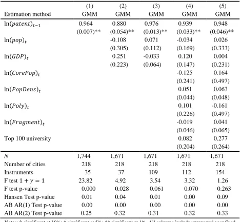
In the Appendix, to check the robustness of our results to the instrument selection process just
described, we report the results of estimating the same specifications as in Table 8, for (1) the
full set of GMM instruments as in Blundell and Bond (1998), and (2) results using bootstrap
resampling of the principal-components-based estimates.
As a first step, we re-estimate equation (6) for the three variables population, GDP and patents
using the GMM method outlined above. The results are reported in columns (4) to (6) of Table
7. Notably, the GMM results are quite different from the fixed-effects results. The standard
errors in all three cases are much larger than those obtained using fixed-effects. This means
that we cannot reject the Gibrat’s Law null hypothesis that 1 +𝛾𝛾 = 1 for all three variables.
That is, we find little evidence of mean reversion in all three variables. That the results are
quite different when the GMM method is used, suggests that the endogeneity of the lagged
dependent variable is an important issue.
< Place Table 8 here >
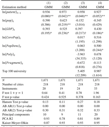
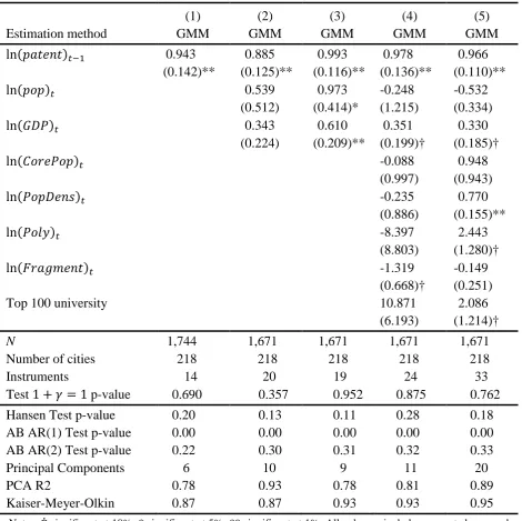
Table 8 presents the results of estimating equation (11), which add additional controls to the
bivariate regression of equation (6). In columns (1) and (2), population and GDP are included.
In column (1), these two variables are assumed to be exogenous, while in column (2) they are
assumed to be endogenous and are instrumented in the same way as the lagged dependent
variable. Including population and GDP results in a slight increase in the size and significance
of the coefficient on lagged patents, when compared with the results in column (6) of Table 7.
Controlling for the endogeneity of the other two variables, in column (2), both population and
17
Columns (3) and (4) include additional controls. This includes the number of local governments
per 100,000 inhabitants of the metropolitan area (capturing the fragmentation of local
government), the number of non-contiguous core areas in the metro area (the polycentricity of
the city), the share of the total metropolitan population living in the core areas of the city, the
population density, and an indicator for whether there is a top-100 university in the city. By
including core population, population density and polycentricity, we seek to explore whether
the concentration of people (Marshall’s knowledge spillovers) affects the degree of innovative
activity. The fragmentation of local government may affect the coordination of government
policies across local governments, which again may influence innovation. In column (3), all
these additional variables are assumed to be exogenous, whereas in column (4), population
density and the share of the total metropolitan population living in the core areas of the city are
treated as endogenous and are instrumented in the usual way.
Including the presence of a top-100 university as an explanatory variable comes from the idea
that knowledge spillovers from university research and research collaborations with local
universities may spur private sector research. Early research on such relationships includes
Jaffe (1989), and more recently Abramovsky et al (2007). There are three major global
university rankings: the Academic Ranking of World Universities (ARWU or the Shanghai
Ranking), the Times Higher Education World University Rankings, and the QS World
University Rankings. The QS World University Rankings were not available for our sample
period, and the other two rankings are available only since 2003 (ARWU) and 2004 (Times).
The results reported below make use of the ARWU rankings in 2008, and we code all cities
with a top-100 university according to this ranking equal to 1, and all other cities equal to zero.
A total of 32 cities in our sample includes at least one top-100 university according to this
18
Once the endogeneity of population density and population share of the core are controlled for
in column (4), population density is positively and significantly associated with patenting
activity. This suggests that if Marshall’s knowledge spillovers are active, one channel via which
they operate is through increased interaction because of greater population density. The other
four additional variables – the degree of polycentricity, the share of metropolitan population
living in the core, the degree of local government fragmentation, and the presence of a top-100
university – do not have statistically significant effects on patenting. Inclusion of these
additional variables leaves the coefficients on lagged patents and GDP unchanged in terms of
both size and significance. However, population is no longer statistically significant in columns
(3) and (4)11. This suggests that, controlling for these additional variables, the level of
economic activity is more strongly associated with innovative activity than the mere presence
of a larger population.
In Table 8, we are unable to reject the null hypothesis of Gibrat’s Law, that 1 +𝛾𝛾 = 1, for all
specifications. That is, there is no evidence of mean reversion; alternatively, we find strong
evidence of persistence in patenting. The results of Table 8 sit somewhat uncomfortably with
the results in previous sections. For instance, in Table 6 in Section 4, the transition probability
matrix showed that patents are persistent at both tails of the distribution, but not in the middle
of the distribution. In Figure 5 in Section 5, the local linear estimates show evidence of
nonlinearity in the relationship between patenting and the growth of patenting. We speculate
that this apparent disparity is due to the fact that the (parametric) approach adopted in this
section restricts the relationship between patents and growth of patents to be linear, whereas
the nonparametric approaches in previous sections are better-able to capture the true
19
We also include a set of diagnostic statistics in Table 8 (similar statistics are reported for the
GMM estimates in columns (4) to (6) of Table 7). First, we report the number of instruments
used, which ranges from 19 to 33 instruments. These are fairly low, which should mitigate the
problem of having too many instruments (see Roodman (2009b))13, and as discussed above, is
because we have used the principal components of the GMM instruments; if we had not done
so, column (4) of Table 8 would have had over 150 instruments. Second, we report the Hansen
test of over-identification. In the baseline column (1), this has a p-value of 0.13, and takes on
similar values as we include additional controls. This suggests reasonable confidence in the
validity of our instruments. A third set of test statistics reported is the Arellano and Bond (1991)
tests for first- and second-order serial correlation in the first-differenced residuals. We find
evidence of first-order serial correlation, but not second-order serial correlation, across all
specifications in Table 8. First-order serial correlation is expected in a dynamic panel; that we
do not find second-order serial correlation provides evidence that our use of lags as instruments
is valid.
7.
CONCLUSIONS
Competition among firms drives innovation in a capitalist economy, as firms seek to gain a
competitive edge over their rivals. Hence as urbanisation proceeds and economic activity
becomes increasingly concentrated in cities, so too does innovative activity. What this paper
has set out to do, is to describe and explain the distribution of innovative activity across OECD
cities. Although there has been much research on innovation in cities, to our knowledge this is
the first paper to compare the distribution of innovation to the distribution of population and
20
Our first main result is that innovation is more highly concentrated than both population and
general economic activity. This is suggestive of the role of Marshall’s knowledge spillovers as
a key driver of innovation. Our second main result is that innovation is less persistent than
population or economic activity, especially in the middle of the distribution. Even in the
relatively short time period in our sample, cities can become much more (or less) innovative.
This gives policymakers hope, that government policy can influence how innovative a city is.
Our third main result is that, even after controlling for the endogeneity of some explanatory
variables, innovation is positively related to general economic activity and population density.
Again this gives policymakers a handle on what types of policies may be more effective at
promoting innovation.
The present paper’s focus on cities as centres of innovative activity yields both advantages and
disadvantages. On the one hand, cities are undoubtedly important; in the OECD, the vast
majority of the population lives and works in cities. So thinking about government policies in
terms of cities may be the more natural unit of analysis. On the other hand, precisely because
cities have not historically been the default unit of analysis, our analysis suffers from data
limitations that not only restrict our sample, but also prevent us from digging deeper into the
determinants of innovative activity as in Audretsch and Feldman (1996, 1999). Such data is
available for different geographical units, and analysis using this data should serve as an
important next step in this line of research. In addition, the use of firm-level data on
productivity and innovation would enable us to present more direct evidence on knowledge
21
Finally, although we find that Gibrat’s Law holds in our sample, more could also be done with
regard to the assumption made, that it makes sense to combine data across major OECD cities.
For instance, the Gibrat’s Law equation (6) could be augmented with a set of country indicators
interacted with lagged city population; this would yield a set of country-specific coefficients,
and a test could be performed for the equality of the country-specific coefficients across
countries. Failure to reject the null of equality would indicate that the relationship between size
and growth is common across countries, and would be supportive of the aggregation of cities
across countries. We have not performed such a test in this paper, since, as shown in Table 1,
each country has a different number of cities in the sample, which represents a different fraction
of each country’s urban population. In this situation, the proposed test may over-reject the null,
as we are not performing a like-for-like comparison between countries. As suggested above,
the use of data for different geographical units may be one way of addressing this issue.
Acknowledgements
Thanks to Geraint Johnes, seminar participants at The Work Foundation, the editor, Jens
Suedekum, and two anonymous referees for helpful suggestions. The author is responsible for
any errors and omissions.
NOTES
1 Are patents an input or an output in the knowledge creation process? Griliches (1990) provides an insightful
discussion on the use of patent statistics in Economics, and concludes that, in the absence of detailed R&D data,
patent data can be used as an indicator of both inventive input and output.
22
2 A simple regression of the natural log of patents against the natural log of population for any one year yields a
coefficient which is always larger than 1; this implies that a 1 percent increase in population has a greater than 1
percent effect on patents. A similar result is obtained for a regression of the natural log of patents against the
natural log of GDP.
3 Some papers in the literature (for instance, Eeckhout, 2004) have suggested that a lognormal distribution may
be more appropriate for city sizes. Along similar lines, Clauset et al (2009) present a set of techniques to validate
and quantify the existence of power laws. We do not pursue these lines of inquiry in this paper.
4 Ioannides and Overman (2001) discuss further the implications of this way of defining 𝐹𝐹
𝑡𝑡 as compared to that
used by Eaton and Eckstein (1997) and Black and Henderson (2003), which is based on fractions of the
contemporaneous mean. In this paper, since we are comparing the distributions of different variables, a
decile-based definition seems more appropriate.
5 Many of the papers which make use of transition probability matrices on city populations go on to obtain the
long run, implied ergodic distribution of city sizes. We do not do so, because the relatively short time period of
our sample means there are relatively few off-diagonal elements of the transition matrices, making the calculations
sensitive to the choice of cell boundaries. In addition, it would require 𝐹𝐹𝑡𝑡 to be defined based on fractions of the
contemporaneous mean (see the previous note) as opposed to our decile-based definition.
6 Because of the many zero entries in the table, it is not possible to perform a chi-squared test of the similarity
between the distributions of the three variables.
7 Equation (5) is of course just the equation that is estimated in a panel unit root test. Conventional panel unit root
tests cannot be used for our data because of the limited time dimension and the fact that we have an unbalanced
panel for GDP. See for instance Bosker et al (2008) for an application of tests of this type to German city sizes.
23
9 We performed a series of sensitivity analyses based on each of the three considerations below. Whilst there are
some differences in the results depending on the choices made, the justification for the results reported is discussed
in the text.
10 Results using the Times ranking are qualitatively similar.
11 This change in results is not driven by the change in sample size between column (2) and column (4).
12 It is of course possible to include nonlinear (quadratic, cubic) terms in the parametric regression analysis.
Exploratory analysis suggested that it is difficult to obtain statistically significant coefficients for the nonlinear
terms. This may indicate that, if nonlinearity does exist in the relationship between size and growth, that the
relationship is more complex than can be captured by the addition of quadratic and cubic terms.
24
REFERENCES
Abramovsky, L., Harrison, R., & Simpson, H. (2007). University research and the location of
business R&D. Economic Journal, 117(519), C114-C141.
Arellano, M. & Bond, S. (1991). Some tests of specification for panel data: Monte Carlo
evidence and an application to employment equations. Review of Economic Studies, 58(2),
277-297.
Audretsch, D.B. & Feldman, M.P. (1996). R&D spillovers and the geography of innovation
and production. American Economic Review, 86(4), 253-273.
Audretsch, D.B. & Feldman, M.P. (1999). Innovation in cities: Science-based diversity,
specialization and localized competition. European Economic Review, 43(2), 409-429.
Audretsch, D.B. & Feldman, M.P. (2004). Knowledge spillovers and the geography of
innovation. In Henderson, J. V. & Thisse, J.-F. (Eds.), Handbook of Regional and Urban
Economics Volume 4 (pp. 2713-2739). Amsterdam: North Holland.
Bai, J. & Ng, S. (2010). Instrumental variable estimation in a data rich environment.
Econometric Theory, 26(6), 1577-1606.
Berry, C.R. and Glaeser, E.L. (2005). The divergence of human capital levels across cities.
25
Bettencourt, L.M.A., Lobo, J., Strumsky, D., & West, G.B. (2010). Urban scaling and its
deviations: Revealing the structure of wealth, innovation and crime across cities. PLoS ONE,
5(11), 1-9.
Bettencourt, L.M.A., Lobo, J., & Strumsky, D. (2007). Invention in the city: Increasing returns
to patenting as a scaling function of metropolitan size. Research Policy, 36(1), 107-120.
Black, D., & Henderson, J.V. (2003). Urban evolution in the USA. Journal of Economic
Geography, 3(4), 343-372.
Blundell, R., & Bond, S. (1998). Initial conditions and moment restrictions in dynamic panel
data models. Journal of Econometrics, 87(1), 115-143.
Bosker, M., Brakman, S., Garretsen, H., & Schramm, M. (2008). A century of shocks: The
evolution of the German city size distribution 1925-1999. Regional Science and Urban
Economics, 38(4), 330-347.
Cameron, A. C., & Trivedi, P.K. (2005). Microeconometrics: Methods and Applications.
Cambridge: Cambridge University Press.
Clauset, A., Shalizi, C.R., & Newman, M.E.J. (2009). Power-law distributions in empirical
data. SIAM Review, 51(4), 661-703.
Cleveland, W.S. (1979). Robust locally weighted regression and smoothing scatterplots.
26
Davis, D.R. & Weinstein, D.E. (2008). A search for multiple equilibria in urban industrial
structure. Journal of Regional Science, 48(1), 29-65.
Dobkins, L.H., & Ioannides, Y.M. (2000). Dynamic evolution of the US city size distribution.
In Huriot, J.-M. & Thisse, J.-F. (Eds.), The Economics of Cities, (pp. 217-260). Cambridge:
Cambridge University Press.
Dobkins, L.H., & Ioannides, Y.M. (2001). Spatial interactions among US cities: 1900-1990.
Regional Science and Urban Economics, 31(6), 701-731.
Eaton, J., & Eckstein, Z. (1997). Cities and growth: Theory and evidence from France and
Japan. Regional Science and Urban Economics, 27(4-5), 443-474.
Eeckhout, J. (2004). Gibrat’s Law for (all) cities. American Economic Review, 94(5),
1429-1451.
Fan, J. (1992). Design-adaptive nonparametric regression. Journal of the American Statistical
Association, 87(420), 998-1004.
Fan, J., & Gijbels, I. (1996). Local polynomial modelling and its applications. London:
Chapman and Hall.
Fujita, M., Krugman, P.R., & Venables, A.J. (1999). The Spatial Economy. Cambridge, MA:
27
Gabaix, X., & Ibragimov, R. (2011). Rank – 1/2: A simple way to improve the OLS estimation
of tail exponents. Journal of Business Economics and Statistics, 29(1), 24-39.
Gabaix, X., & Ioannides, Y.M. (2004). The evolution of city size distributions. In Henderson,
J. V., & Thisse, J.-F. (Eds.), Handbook of Regional and Urban Economics, Volume 4, (pp.
2341-2379). Amsterdam: North Holland.
Glaeser, E.L., Kallal, H.D., Scheinkman, J.A., & Shleifer, A. (1992). Growth in cities. Journal
of Political Economy, 100(6), 1126-1152.
Glaeser, E.L., Scheinkman, J.A., & Shleifer, A. (1995). Economic growth in a cross-section of
cities. Journal of Monetary Economics, 36(1), 117-143.
Griliches, Z. (1990). Patent statistics as economic indicators: A survey. Journal of Economic
Literature, 28(4), 1661-1707.
Hansen, B.E. (2017). Econometrics. Unpublished manuscript, University of Wisconsin.
Ioannides, Y.M., & Overman, H.G. (2004). Spatial evolution of the US urban system. Journal
of Economic Geography, 4(2), 131-156.
Ioannides, Y.M., & Overman, H.G. (2003). Zipf’s Law for cities: An empirical examination.
28
Ioannides, Y.M., & Overman, H.G. (2001). Cross-sectional exolution of the US city size
distribution. Journal of Urban Economics, 49(3), 543-566.
Jaffe. A.B. (1989). Real effects of academic research. American Economic Review, 79(5),
957-970.
Kapetanios, G., & Marcellino, M. (2010). Factor-GMM estimation with large sets of possibly
weak instruments. Computational Statistics and Data Analysis, 54(11), 2655-2675.
Krugman, P.R. (1991). Geography and Trade. Cambridge, MA: MIT Press.
Marshall, A. (1920). Principles of Economics (8th Edition). London: MacMillan.
Mehrhoff, J. (2009). A solution to the problem of too many instruments in dynamic panel data
GMM (Discussion Paper 200931). Frankfurt: Deutsche Bundesbank.
OECD (2012). Redefining “Urban”: A new way to measure metropolitan areas. Paris: OECD
Publishing.
OhUallachain, B. (1999). Patent places: Size matters. Journal of Regional Science, 39(4),
613-636.
Quah, D. (1993). Empirical cross-section dynamics in economic growth. European Economic
29
Roodman, D. (2009a). How to do xtabond2: An introduction to ‘difference’ and ‘system’
GMM in Stata. Stata Journal, 9(1), 86-136.
Roodman, D. (2009b). A note on the theme of too many instruments. Oxford Bulletin of
Economics and Statistics, 71(1), 135-158.
Silverman, B. (1986). Density estimation for statistics and data analysis. London: Chapman
and Hall.
Soo, K.T. (2005). Zipf’s Law for cities: A cross-country investigation. Regional Science and
Urban Economics, 35(3), 239-263.
Soo, K.T. (2007). Zipf’s Law and urban growth in Malaysia. Urban Studies, 44(1), 1-14.
Strumsky, D., & Thill, J.-C. (2013). Profiling US metropolitan regions by their social research
networks and regional economic performance. Journal of Regional Science, 53(5), 813-833.
Wand, M.P., & Jones, M.C. (1995). Kernel smoothing. New York: Chapman and Hall.
Windmeijer, F. (2005). A finite sample correction for the variance of linear efficient two-step
GMM estimators. Journal of Econometrics, 126(1), 25-51.
Zipf, G.K. (1949). Human behaviour and the principle of least effort. Cambridge, MA:
30
TABLE 1: Distribution of cities across countries in the sample
Country Number of cities Country Number of cities
Austria 3 Japan 36
Belgium 4 Mexico 31
Denmark 1 Netherlands 5
Estonia 1 Norway 1
Finland 1 Portugal 2
France 15 Spain 8
Germany 24 Sweden 3
Italy 11 United States 72
[image:31.595.155.438.344.415.2]Total 218
TABLE 2: Correlation between patents, GDP and population, 2008 (N = 218)
Patents GDP Population
Patents 1.000
GDP 0.833 1.000
Population 0.797 0.939 1.000
TABLE 3: Top 10 cities with the largest number of patents in 2008
City Population Rank Patents Rank GDP Rank
Tokyo 34,482,744 1(1) 8,727.0 1(2) 1,316,049 1(-)
San Francisco 6,778,659 10(10) 5,138.2 2(1) 463,435 7(5)
Osaka 17,211,140 4(4) 4,451.1 3(4) 534,747 5(-)
San Diego 3,036,850 35(37) 2,689.3 4(10) 160,635 23(18)
Paris 11,529,670 7(7) 2,467.6 5(7) 575,983 4(3)
Boston 3,616,814 29(28) 2,207.5 6(3) 241,083 12(8)
New York 16,453,331 6(5) 2,001.7 7(6) 977,119 2(1)
Los Angeles 16,742,427 5(6) 1,957.7 8(5) 768,032 3(2)
Minneapolis 3,212,176 34(34) 1,672.5 9(11) 174,234 18(16)
Houston 5,363,803 16(17) 1,590.1 10(16) 323,819 9(7)
[image:31.595.71.527.496.678.2]31
TABLE 4: Descriptive statistics for population, GDP and patents
Variable N Mean Std. Dev.
ln (𝑝𝑝𝑝𝑝𝑝𝑝) 1,332 14.04 0.7547 ln (𝐺𝐺𝐺𝐺𝐺𝐺) 1,332 10.75 0.9210 ln (𝑝𝑝𝑎𝑎𝑡𝑡𝑝𝑝𝑛𝑛𝑡𝑡) 1,332 4.906 1.3876
Notes: Statistics reported for a consistent sample of 148 cities for which complete data are available from 2000 to 2008.
TABLE 5: Zipf regressions for population, GDP and patents, by year
(1) (2) (3)
Year Population GDP Patents
[image:32.595.126.475.281.606.2]2000 1.246 1.041 0.330
(0.119)* (0.121) (0.032)**
2001 1.247 1.026 0.350
(0.119)* (0.107) (0.033)**
2002 1.248 1.025 0.375
(0.119)* (0.107) (0.036)**
2003 1.247 0.927 0.358
(0.119)* (0.089) (0.034)**
2004 1.248 0.927 0.370
(0.119)* (0.089) (0.035)**
2005 1.247 0.926 0.384
(0.119)* (0.089) (0.037)**
2006 1.246 0.928 0.387
(0.119)* (0.089) (0.037)**
2007 1.245 0.928 0.397
(0.119)* (0.089) (0.038)**
2008 1.244 0.932 0.426
(0.119)* (0.089) (0.041)**
Notes: † significant at 10%; * significant at 5%; ** significant at 1%. Statistical significance is in terms of the
32
TABLE 6: Transition probability matrices for population, GDP and patents, 2000-2008
2000 2008 0.1 0.2 0.3 0.4 0.5 0.6 0.7 0.8 0.9 1.0
0.1 Pop 71.4 25.0 3.6 0.0 0.0 0.0 0.0 0.0 0.0 0.0
GDP 85.7 14.3 0.0 0.0 0.0 0.0 0.0 0.0 0.0 0.0
Patent 86.4 13.6 0.0 0.0 0.0 0.0 0.0 0.0 0.0 0.0
0.2 Pop 25.9 51.9 18.5 3.7 0.0 0.0 0.0 0.0 0.0 0.0
GDP 15.0 65.0 15.0 5.0 0.0 0.0 0.0 0.0 0.0 0.0
Patent 13.6 63.6 22.7 0.0 0.0 0.0 0.0 0.0 0.0 0.0
0.3 Pop 0.0 17.9 53.6 28.6 0.0 0.0 0.0 0.0 0.0 0.0
GDP 0.0 20.0 55.0 15.0 10.0 0.0 0.0 0.0 0.0 0.0
Patent 0.0 13.6 36.4 31.8 9.1 9.1 0.0 0.0 0.0 0.0
0.4 Pop 0.0 0.0 25.9 48.2 25.9 0.0 0.0 0.0 0.0 0.0
GDP 0.0 0.0 25.0 55.0 20.0 0.0 0.0 0.0 0.0 0.0
Patent 0.0 4.6 18.2 18.2 22.7 27.3 4.6 4.6 0.0 0.0
0.5 Pop 3.6 0.0 0.0 17.9 67.9 10.7 0.0 0.0 0.0 0.0
GDP 0.0 0.0 5.0 25.0 65.0 5.0 0.0 0.0 0.0 0.0
Patent 0.0 4.8 14.3 38.1 28.6 14.3 0.0 0.0 0.0 0.0
0.6 Pop 0.0 3.7 0.0 0.0 7.4 66.7 22.2 0.0 0.0 0.0
GDP 0.0 0.0 0.0 0.0 4.8 85.7 9.5 0.0 0.0 0.0
Patent 0.0 0.0 9.1 4.6 27.3 31.8 27.3 0.0 0.0 0.0
0.7 Pop 0.0 0.0 0.0 0.0 0.0 21.4 64.3 14.3 0.0 0.0
GDP 0.0 0.0 0.0 0.0 0.0 10.0 65.0 25.0 0.0 0.0
Patent 0.0 0.0 0.0 9.1 9.1 18.2 36.4 22.7 4.6 0.0
0.8 Pop 0.0 0.0 0.0 0.0 0.0 0.0 14.8 81.5 3.7 0.0
GDP 0.0 0.0 0.0 0.0 0.0 0.0 25.0 55.0 20.0 0.0
Patent 0.0 0.0 0.0 0.0 0.0 0.0 31.8 54.6 13.6 0.0
0.9 Pop 0.0 0.0 0.0 0.0 0.0 0.0 0.0 3.6 89.3 7.1
GDP 0.0 0.0 0.0 0.0 0.0 0.0 0.0 20.0 75.0 5.0
Patent 0.0 0.0 0.0 0.0 0.0 0.0 0.0 18.2 68.2 13.6
1.0 Pop 0.0 0.0 0.0 0.0 0.0 0.0 0.0 0.0 7.4 92.6
GDP 0.0 0.0 0.0 0.0 0.0 0.0 0.0 0.0 5.0 95.0
Patent 0.0 0.0 0.0 0.0 0.0 0.0 0.0 0.0 14.3 85.7
33 TABLE 7: Test of Gibrat’s Law
(1) (2) (3) (4) (5) (6)
Variable Population GDP Patents Population GDP Patents
Estimation method FE FE FE GMM GMM GMM
ln(𝑝𝑝𝑝𝑝𝑝𝑝𝑝𝑝𝑝𝑝𝑎𝑎𝑡𝑡𝑖𝑖𝑝𝑝𝑛𝑛)𝑡𝑡−1 0.919 0.969
(0.035)** (0.350)**
ln(𝐺𝐺𝐺𝐺𝐺𝐺)𝑡𝑡−1 0.897 0.654
(0.020)** (0.317)*
ln(𝑝𝑝𝑎𝑎𝑡𝑡𝑝𝑝𝑛𝑛𝑡𝑡)𝑡𝑡−1 0.186 0.912
(0.058)** (0.137)**
R2 0.99 0.90 0.31
N 2,200 2,033 1,744 2,200 2,033 1,744
Cities 275 271 218 275 271 218
F-test 1 +𝛾𝛾 = 1 5.34 25.67 198.96 0.01 1.19 0.41
F-test p-value 0.022 0.000 0.000 0.930 0.276 0.522
Instruments 17 14 14
Hansen Test p-value 0.00 0.29 0.20
AB AR(1) Test p-value 0.94 0.06 0.00
AB AR(2) Test p-value 0.94 0.10 0.22
Principal Components 8 5 6
PCA R2 0.84 0.67 0.78
Kaiser-Meyer-Olkin 0.83 0.81 0.87
Notes: † significant at 10%; * significant at 5%; ** significant at 1%. All columns include unreported year and city fixed effects, and the sample covers the time period from
34
TABLE 8: The determinants of patenting activity (dependent variable: ln(𝑝𝑝𝑎𝑎𝑡𝑡𝑝𝑝𝑛𝑛𝑡𝑡)𝑡𝑡)
(1) (2) (3) (4)
Estimation method GMM GMM GMM GMM
ln(𝑝𝑝𝑎𝑎𝑡𝑡𝑝𝑝𝑛𝑛𝑡𝑡)𝑡𝑡−1 0.936 0.973 0.958 0.927
(0.080)** (0.042)** (0.048)** (0.052)**
ln(𝑝𝑝𝑝𝑝𝑝𝑝)𝑡𝑡 0.390 0.623 -0.152 -0.345
(0.386) (0.219)** (3.014) (0.429)
ln(𝐺𝐺𝐺𝐺𝐺𝐺)𝑡𝑡 0.393 0.525 0.397 0.430
(0.195)* (0.236)* (0.217)† (0.186)*
ln(𝐶𝐶𝑝𝑝𝐶𝐶𝑝𝑝𝐺𝐺𝑝𝑝𝑝𝑝)𝑡𝑡 0.017 0.516
(1.195) (1.298)
ln(𝐺𝐺𝑝𝑝𝑝𝑝𝐺𝐺𝑝𝑝𝑛𝑛𝑃𝑃)𝑡𝑡 0.063 0.500
(3.200) (0.244)*
ln(𝐺𝐺𝑝𝑝𝑝𝑝𝑃𝑃)𝑡𝑡 -3.963 0.678
(34.333) (3.120)
ln(𝐹𝐹𝐶𝐶𝑎𝑎𝐹𝐹𝑚𝑚𝑝𝑝𝑛𝑛𝑡𝑡)𝑡𝑡 -0.672 -0.113
(0.818) (0.276)
Top 100 university 5.405 0.987
(12.209) (1.614)
N 1,671 1,671 1,671 1,671
Number of cities 218 218 218 218
Instruments 20 19 24 33
F test 1 +𝛾𝛾 = 1 0.64 0.41 0.78 1.96
F test p-value 0.424 0.525 0.378 0.163
Hansen Test p-value 0.13 0.11 0.27 0.18
AB AR(1) Test p-value 0.00 0.00 0.00 0.00
AB AR(2) Test p-value 0.30 0.31 0.32 0.33
Principal components 10 9 11 20
PCA R2 0.93 0.78 0.81 0.89
Kaiser-Meyer-Olkin 0.87 0.93 0.93 0.95
Notes: † significant at 10%; * significant at 5%; ** significant at 1%. All columns include unreported year and
city fixed effects. Estimation is via the two-step Blundell-Bond (1998) System GMM with Windmeijer (2005) corrected standard errors. 𝐶𝐶𝑝𝑝𝐶𝐶𝑝𝑝𝐺𝐺𝑝𝑝𝑝𝑝 is the concentration of population in the metropolitan core. 𝐺𝐺𝑝𝑝𝑝𝑝𝐺𝐺𝑝𝑝𝑛𝑛𝑃𝑃 is population density. 𝐺𝐺𝑝𝑝𝑝𝑝𝑃𝑃 is the degree of polycentricity of the city. 𝐹𝐹𝐶𝐶𝑎𝑎𝐹𝐹𝑚𝑚𝑝𝑝𝑛𝑛𝑡𝑡 is the degree of fragmentation of local government. Top 100 university is an indicator for whether there is a top-100 university in the city, as ranked
35
FIGURE 1: Scatterplot of patent applications, population and real GDP, 2008 (N = 218)
Patent applications and population.
Patent applications and real GDP.
FIGURE 2: Coefficient of variation for population, GDP and patents, for a consistent sample
of 148 cities, 2000-2008
1 10 10 0 10 00 10 00 0 P at en t ap pl ic at io ns ( c o un t)
500 1000 2000 4000 8000 16000 Total population metro area (thousand persons)
1 10 10 0 10 00 10 00 0 P at en t ap pl ic at io ns ( c o un t)
2000 20000 200000 200000 GDP (millions US$)
0 0.05 0.1 0.15 0.2 0.25 0.3 0.35
2000 2001 2002 2003 2004 2005 2006 2007 2008
Co effic ie nt o f v ar ia tio n
[image:36.595.116.480.385.601.2]36
FIGURE 3: Kernel density functions for population, GDP and patents, for 2008, log scale
Notes: Epanechnikov kernel used. Bandwidth is the Silverman (1986) rule-of-thumb bandwidth. Bandwidth = 0.2254 for population, bandwidth = 0.3106 for GDP, bandwidth = 0.4393 for patents.
FIGURE 4: Zipf plots of population, patents and GDP, for 2008, log scale, normalised to the
size of the largest city
0
.2
.4
.6
.8
0 5 10 15 20
ln(pop) ln(GDP)
ln(patent)
1
2
4
8
16
32
64
128
256
R
ank
.0001 .001 .01 .1 1
Relative size
[image:37.595.121.477.486.738.2]37
FIGURE 5: Nonparametric local linear estimates of the relationship between city size and city
growth
Notes: The shaded area indicates the 95% confidence interval. Bandwidth indicates the bandwidth used for the smoothing, while pwidth = 1.5*bandwidth indicates the bandwidth used for the confidence interval. See the text for more details.
-. 3 -. 2 -. 1 0 .1 .2 S ta nd ar di s ed po pu lat ion g row th
-2 -1 0 1 2 3 4
Standardised population, log scale
kernel = epanechnikov, degree = 1, bandwidth = .61, pwidth = .91
Population -1 0 1 2 3 S tan da rd is e d p at en t gr ow th
-3 -2 -1 0 1 2
Standardised patents, log scale
kernel = epanechnikov, degree = 1, bandwidth = .2, pwidth = .31
Patents -. 5 0 .5 1 S ta nd ar di s ed G D P gr ow th
-3 -2 -1 0 1 2 3 4
Standardised GDP, log scale
kernel = epanechnikov, degree = 1, bandwidth = .69, pwidth = 1.03
38
Appendix: Additional results for the determinants of patenting activity
In Section 6, the results were presented using the Blundell and Bond (1998) system GMM
method, with the instruments used being the principal components of the GMM instruments,
to avoid the problem of too many instruments (Roodman, 2009b). However, this may raise
questions about the robustness of the inferences made. In this Appendix, we report two
additional results to those reported in Section 6. First, as reported in Table A1, we use the
standard GMM instruments instead of the principal components of the GMM instruments.
Second, as reported in Table A2, we employ bootstrap resampling methods on the principal
components estimates. One thousand replications were performed, with the sample drawn in
each replication being a bootstrap sample of cities (i.e. a block bootstrap is used). The results
reported in Table A2, in addition to the bootstrapped standard errors, also include a bias
correction obtained from the difference between the bootstrap estimates and the GMM
estimates reported in Table 8 (see, for instance, Cameron and Trivedi, 2005).
Comparing the results of Table A1 with those of Table 8, using the standard GMM instruments
in Table A1 results in a large number of instruments; over 100 in columns (3) to (5). This may
give rise to the problem of too many instruments. The use of the principal components of the
GMM instruments in Table 8 results in similar performance of the Arellano and Bond (1991)
tests, and superior performance of the Hansen test of overidentifying restrictions. In Table 8,
we never reject the null hypothesis of overidentification at conventional significance levels,
but in Table A1 we reject the null four out of five times. The coefficients on the lagged
dependent variable are of similar orders of magnitude, although in Table A1 there is a slightly
higher likelihood of rejecting the null hypothesis of Gibrat’s Law. In addition, in Table 8 we
39
density, which we are unable to in Table A1. Overall, we interpret Table A1 as indicating that
using the full set of GMM instruments may lead to incorrect inferences because of the presence
of too many instruments, hence justifying the use of the principal components reduction of the
instrument set in the text.
The results reported in Table A2 with bootstrap resampling are broadly comparable with those
in Table 8, in terms of both the estimated coefficients, and the specification tests. We never
statistically reject the Gibrat’s Law hypothesis that 1 +𝛾𝛾 = 1. In column (5), which is
comparable to column (4) in Table 8, GDP and population density are positively and
significantly associated with patents. In addition, the presence of a top 100 university and how
polycentric the city is, are now positively associated with patents. The positive association
between the presence of a top university and patenting is perhaps unsurprising. That a more
polycentric city is more innovative, controlling for other variables such as population density,
40
TABLE A1: The determinants of patenting activity (dependent variable: ln(𝑝𝑝𝑎𝑎𝑡𝑡𝑝𝑝𝑛𝑛𝑡𝑡)𝑡𝑡): Full set
of GMM instruments
(1) (2) (3) (4) (5)
Estimation method GMM GMM GMM GMM GMM
ln(𝑝𝑝𝑎𝑎𝑡𝑡𝑝𝑝𝑛𝑛𝑡𝑡)𝑡𝑡−1 0.964 0.880 0.976 0.939 0.948
(0.007)** (0.054)** (0.013)** (0.033)** (0.046)**
ln(𝑝𝑝𝑝𝑝𝑝𝑝)𝑡𝑡 -0.108 0.071 -0.034 0.026
(0.305) (0.112) (0.169) (0.333)
ln(𝐺𝐺𝐺𝐺𝐺𝐺)𝑡𝑡 0.251 -0.033 0.120 0.004
(0.223) (0.064) (0.147) (0.231)
ln(𝐶𝐶𝑝𝑝𝐶𝐶𝑝𝑝𝐺𝐺𝑝𝑝𝑝𝑝)𝑡𝑡 -0.125 0.164
(0.241) (0.497)
ln(𝐺𝐺𝑝𝑝𝑝𝑝𝐺𝐺𝑝𝑝𝑛𝑛𝑃𝑃)𝑡𝑡 0.051 0.063
(0.044) (0.048)
ln(𝐺𝐺𝑝𝑝𝑝𝑝𝑃𝑃)𝑡𝑡 0.101 -0.161
(0.226) (0.497)
ln(𝐹𝐹𝐶𝐶𝑎𝑎𝐹𝐹𝑚𝑚𝑝𝑝𝑛𝑛𝑡𝑡)𝑡𝑡 -0.019 0.041
(0.046) (0.065)
Top 100 university 0.082 0.277
(0.204) (0.264)
N 1,744 1,671 1,671 1,671 1,671
Number of cities 218 218 218 218 218
Instruments 35 37 109 112 154
F test 1 +𝛾𝛾= 1 23.82 4.92 3.54 3.32 1.26
F test p-value 0.000 0.028 0.061 0.070 0.263
Hansen Test p-value 0.01 0.04 0.01 0.00 0.09
AB AR(1) Test p-value 0.00 0.00 0.00 0.00 0.00
AB AR(2) Test p-value 0.25 0.32 0.31 0.32 0.33
Notes: † significant at 10%; * significant at 5%; ** significant at 1%. All columns include unreported year fixed
effects. Estimation is via the two-step Blundell-Bond (1998) System GMM with Windmeijer (2005) corrected