Word Reordering and a Dynamic Programming Beam Search Algorithm for Statistical Machine Translation

Programming Beam Search Algorithm for

Statistical Machine Translation

Christoph Tillmann

_{Hermann Ney}

IBM T. J. Watson Research Center RWTH Aachen

In this article, we describe an efficient beam search algorithm for statistical machine translation based on dynamic programming (DP). The search algorithm uses the translation model presented in Brown et al. (1993). Starting from a DP-based solution to the traveling-salesman problem, we present a novel technique to restrict the possible word reorderings between source and target language in order to achieve an efficient search algorithm. Word reordering restrictions especially useful for the translation direction German to English are presented. The restrictions are gener-alized, and a set of four parameters to control the word reordering is introduced, which then can easily be adopted to new translation directions. The beam search procedure has been successfully tested on the Verbmobil task (German to English, 8,000-word vocabulary) and on the Canadian Hansards task (French to English, 100,000-word vocabulary). For the medium-sized Verbmobil task, a sentence can be translated in a few seconds, only a small number of search errors occur, and there is no performance degradation as measured by the word error criterion used in this article.

1. Introduction

This article is about a search procedure for statistical machine translation (MT). The task of the search procedure is to find the most likely translation given a source sen-tence and a set of model parameters. Here, we will use a trigram language model and the translation model presented in Brown et al. (1993). Since the number of possible translations of a given source sentence is enormous, we must find the best output without actually generating the set of all possible translations; instead we would like to focus on the most likely translation hypotheses during the search process. For this purpose, we present a data-driven beam search algorithm similar to the one used in speech recognition search algorithms (Ney et al. 1992). The major difference between the search problem in speech recognition and statistical MT is that MT must take into account the different word order for the source and the target language, which does not enter into speech recognition. Tillmann, Vogel, Ney, and Zubiaga (1997) proposes a dynamic programming (DP)–based search algorithm for statistical MT that mono-tonically translates the input sentence from left to right. The word order difference is dealt with using a suitable preprocessing step. Although the resulting search proce-dure is very fast, the preprocessing is language specific and requires a lot of manual

∗IBM T. J. Watson Research Center, Yorktown Heights, NY 10598. E-mail: ctill@us.ibm.com. The research reported here was carried out while the author was with Lehrstuhl f ¨ur Informatik VI, Computer Science Department, RWTH Aachen.

work. Currently, most search algorithms for statistical MT proposed in the literature are based on theA∗ concept (Nilsson 1971). Here, the word reordering can be easily included in the search procedure, since the input sentence positions can be processed in any order. The work presented in Berger et al. (1996) that is based on theA∗concept, however, introduces word reordering restrictions in order to reduce the overall search space.

The search procedure presented in this article is based on a DP algorithm to solve the traveling-salesman problem (TSP). A data-driven beam search approach is pre-sented on the basis of this DP-based algorithm. The cities in the TSP correspond to source positions of the input sentence. By imposing constraints on the possible word reorderings similar to that described in Berger et al. (1996), the DP-based approach becomes more effective: when the constraints are applied, the number of word re-orderings is greatly reduced. The original reordering constraint in Berger et al. (1996) is shown to be a special case of a more general restriction scheme in which the word reordering constraints are expressed in terms of simple combinatorical restrictions on the processed sets of source sentence positions.1 _{A set of four parameters is given to} control the word reordering. Additionally, a set of four states is introduced to deal with grammatical reordering restrictions (e.g., for the translation direction German to English, the word order difference between the two languages is mainly due to the German verb group. In combination with the reordering restrictions, a data-driven beam search organization for the search procedure is proposed. A beam search prun-ing technique is conceived that jointly processes partial hypotheses accordprun-ing to two criteria: (1) The partial hypotheses cover the same set of source sentence positions, and (2) the partial hypotheses cover setsC of source sentence positions of equal car-dinality. A partial hypothesis is said to covera set of source sentence positions when exactly the positions in the set have already been processed in the search process. To verify the effectiveness of the proposed techniques, we report and analyze results for two translation tasks: the German to English Verbmobil task and French to English Canadian Hansards task.

The article is structured as follows. Section 2 gives a short introduction to the trans-lation model used and reports on other approaches to the search problem in statistical MT. In Section 3, a DP-based search approach is presented, along with appropriate pruning techniques that yield an efficient beam search algorithm. Section 4 reports and analyzes translation results for the different translation directions. In Section 5, we conclude with a discussion of the achieved results.

2. Previous Work

2.1 IBM Translation Approach

In this article, we use the translation model presented in Brown et al. (1993), and the mathematical notation we use here is taken from that paper as well: a source string f₁J =f1· · ·fj· · ·fJ is to be translated into a target stringeI1 =e1· · ·ei· · ·eI. Here, Iis the

length of the target string, andJis the length of the source string. Among all possible target strings, we will choose the string with the highest probability as given by Bayes’

Figure 1

Architecture of the statistical translation approach based on Bayes’ decision rule.

decision rule:

ˆeI₁ = arg max

eI

1

{Pr(eI₁|f₁J)}

= arg max

eI

1

{Pr(eI₁)·Pr(f₁J |eI₁)} (1)

Pr(eI

1)is the language model of the target language, whereas Pr(f

J

catego-rization as an explicit transformation step. In the search procedure both the language and the translation model are appliedafterthe text transformation steps. The following “types” of parameters are used for the IBM-4 translation model:

Lexicon probabilities: We use the lexicon probability p(f | e)for translating the single target word e as the single source word f. A source word f may be translated by the “null” word e0 (i.e., it does not produce any target worde). A translation probabilityp(f |e0)is trained along with the regular translation probabilities.

Fertilities: A single target wordemay be aligned ton=0, 1 or more source words. This is explicitly modeled by the fertility parameterφ(n|e): the probability that the target word e is translated by n source words is φ(n | e). The fertility for the “null” word is treated specially (for details see Brown et al. [1993]). Berger et al. (1996) describes the extension of a partial hypothesis by a pair of target words (e,e), where e is not connected to any source wordf. In this case, the so-called spontaneous target wordeis accounted for with the fertility. Here, the translation probability φ(0 | e) and no-translation probabilityp(f |e).

Class-based distortion probabilities: When covering a source sentence position j, we use distortion probabilities that depend on the previously covered source sentence positions (we say that a source sentence positionjis cov-ered for a partial hypothesis when it is taken account of in the translation process by generating a target word or the “null” worde0 ). In Brown et al. (1993), two types of distortion probabilities are distinguished: (1) the leftmost word of a set of source wordsf aligned to the same target word e (which is called the “head”) is placed, and (2) the remaining source words are placed. Two separate distributions are used for these two cases. For placing the “head” the center function center(i)(Brown et al. [1993] uses the notation i) is used: the average position of the source words

with which the target word ei−1 is aligned. The distortion probabilities are class-based: They depend on the word classF(f)of a covered source wordf as well as on the word classE(e)of the previously generated target worde. The classes are automatically trained (Brown et al. 1992).

2.2 Search Algorithms for Statistical Machine Translation

In this section, we give a short overview of search procedures used in statistical MT: Brown et al. (1990) and Brown et al. (1993) describe a statistical MT system that is based on the same statistical principles as those used in most speech recognition systems (Jelinek 1976). Berger et al. (1994) describes the French-to-English Candide translation system, which uses the translation model proposed in Brown et al. (1993). A detailed description of the decoder used in that system is given in Berger et al. (1996) but has never been published in a paper: Throughout the search process, partial hypotheses are maintained in a set of priority queues. There is a single priority queue for each subset of covered positions in the source string. In practice, the priority queues are initialized only on demand; far fewer than the full number of queues possible are actu-ally used. The priority queues are limited in size, and only the 1,000 hypotheses with the highest probability are maintained. Each priority queue is assigned a threshold to select the hypotheses that are going to be extended, and the process of assigning these thresholds is rather complicated. A restriction on the possible word reorderings, which is described in Section 3.6, is applied.

Wang and Waibel (1997) presents a search algorithm for the IBM-2 translation model based on the A∗ concept and multiple stacks. An extension of this algorithm is demonstrated in Wang and Waibel (1998). Here, a reshuffling step on top of the original decoder is used to handle more complex translation models (e.g., the IBM-3 model is added). Translation approaches that use the IBM-2 model parameters but are based on DP are presented in Garc´ıa-Varea, Casacuberta, and Ney (1998) and Niessen et al. (1998). An approach based on the hidden Markov model alignments as used in speech recognition is presented in Tillmann, Vogel, Ney, and Zubiaga (1997) and Tillmann, Vogel, Ney, Zubiaga, and Sawaf (1997). This approach assumes that source and target language have the same word order, and word order differences are dealt with in a preprocessing stage. The work by Wu (1996) also uses the original IBM model parameters and obtains an efficient search algorithm by restricting the possible word reorderings using the so-called stochastic bracketing transduction grammar.

Three different decoders for the IBM-4 translation model are compared in Germann et al. (2001). The first is a reimplementation of the stack-based decoder described in Berger et al. (1996). The second is a greedy decoder that starts with an approximate solution and then iteratively improves this first rough solution. The third converts the decoding problem into an integer program (IP), and a standard software package for solving IP is used. Although the last approach is guaranteed to find the optimal solution, it is tested only for input sentences of length eight or shorter.

This article will present a DP-based beam search decoder for the IBM-4 translation model. The decoder is designed to carry out an almost full search with a small number of search errors and with little performance degradation as measured by the word error criterion. A preliminary version of the work presented here was published in Tillmann and Ney (2000).

3. Beam Search in Statistical Machine Translation

3.1 Inverted Alignment Concept

To explicitly describe the word order difference between source and target language, Brown et al. (1993) introduced an alignment concept, in which a source position jis mapped to exactly one target positioni:

e

.

In

this

case

my

colleague

can

k

not

visit

on

the

fourth

of

May

m K S

you

a v M n

c

h

t

b

F

e

s

u

c

h

e

n

.

n

d

e

a

n

n

o

e

g

e

e

e

n

i

a

i

I

i

i

i

m

e

s

i

r

t

e

l

l

l

l

a

m

n

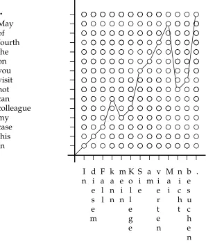
Regular alignment example for the translation direction German to English. For each German source word there is exactly one English target word on the alignment path.

An example for this kind of alignment is given in Figure 2, in which each German source positionjis mapped to an English target positioni. In Brown et al. (1993), this alignment concept is used for model IBM-1 through model IBM-5. For search purposes, we use the inverted alignment concept as introduced in Niessen et al. (1998) and Ney et al. (2000). An inverted alignment is defined as follows:

inverted alignment: i→j=bi

Here, a target position iis mapped to a source position j. Thecoverage constraint for an inverted alignment is not expressed by the notation: Each source positionjshould be “hit” exactly once by the path of the inverted alignment bI

1 = b1· · ·bi· · ·bI. The

Figure 3

Illustration of the transitions in the regular and in the inverted alignment model. The regular alignment model (left figure) is used to generate the sentence from left to right; the inverted alignment model (right figure) is used to generate the sentence from bottom to top.

sentenceeI

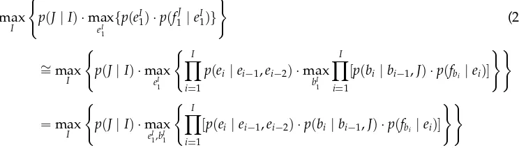
1 of lengthI=Jfor an observed source sentence f1J of length J:

max

I

p(J|I)·max

eI

1

{p(eI

1)·p(f1J |eI1)}

(2)

∼

=max

I

p(J|I)·max

eI

1

_I

i=1

p(ei|ei−1,ei−2)·max

bI

1

I

i=1

[p(bi|bi−1,J)·p(fbi|ei)]

=max

I

p(J|I)·max

eI

1,bI1

_I

i=1

[p(ei|ei−1,ei−2)·p(bi|bi−1,J)·p(fbi |ei)]

The following notation is used:ei−1,ei−2 are the immediate predecessor target words, eiis the word to be hypothesized,p(ei|ei−1,ei−2)denotes the trigram language model probability, p(fbi |ei)denotes the lexicon probability for translating the target word ei as source word fbi, and p(bi | bi−1,J)is the distortion probability for covering source positionbiafter source positionbi−1. Note that in equation (2) two products overiare merged into a single product overi. The translation probabilityp(f₁J |eI

1)is computed in the maximum approximation using the distortion and the lexicon probabilities. Finally, p(J|I)is the sentence length model, which will be dropped in the following (it is not used in the IBM-4 translation model). For each source sentencef₁J to be translated, we are searching for the unknown mapping that optimizes equation (2):

i→(bi,ei)

Table 1

DP-based algorithm for solving traveling-salesman problems due to Held and Karp. The outermost loop is over the cardinality of subsets of already visited cities.

input: citiesj=1,. . .,Jwith distance matrixdjj initialization:D({k},k):=d1k

for each path lengthc=2,. . .,Jdo

for each pair(C,j), whereC ⊆ {2,. . .,J}andj∈ C and|C|=cdo

D(C,j) = min

j∈C\{j}{djj+D(C\{j},j _)}

traceback:

•find shortest tour:D∗= min

k∈{2,...,J}[D({2,. . .,J},k) +dk1]

•recover optimal sequence of cities

translation lattice, the unknown target word sequence can be obtained by tracing back the translation decisions to the partial hypothesis at stage i=1. The grid points are defined in Section 3.3. In the left part of the figure the regular alignment concept is shown for comparison purposes.

3.2 Held and Karp Algorithm for Traveling-Salesman Problem

Held and Karp (1962) presents a DP approach to solve the TSP, an optimization prob-lem that is defined as follows: Given are a set of cities {1,. . .,J} and for each pair of cities j,j the cost djj > 0 for traveling from city j to city j. We are looking for

the shortest tour, starting and ending in city 1, that visits all cities in the set of cities exactly once. We are using the notationC for the set of cities, since it corresponds to a coverage set of processed source positions in MT. A straightforward way to find the shortest tour is by trying all possible permutations of the J cities. The resulting algorithm has a complexity ofO(J!). DP can be used, however, to find the shortest tour inO(J2_·2J_{), which is a much smaller complexity for larger values ofJ. The approach}

recursively evaluates the quantityD(C,j):

D(C,j) := costs of the partial tour starting in city 1, ending in cityj, and visiting all cities inC

Subsets of cities C of increasing cardinalitycare processed. The algorithm, shown in Table 1, works because not all permutations of cities have to be considered explicitly. During the computation, for a pair(C,j), the order in which the cities inC have been visited can be ignored (exceptj); only the costs for the best path reachingj has to be stored. For the initialization the costs for starting from city 1 are set:D({k},k) =d1kfor

each k∈ {2,. . .,|C|}. Then, subsets C of increasing cardinality are processed. Finally, the cost for the optimal tour is obtained in the second-to-last line of the algorithm. The optimal tour itself can be found using a back-pointer array in which the optimal decision for each grid point (C,j)is stored.

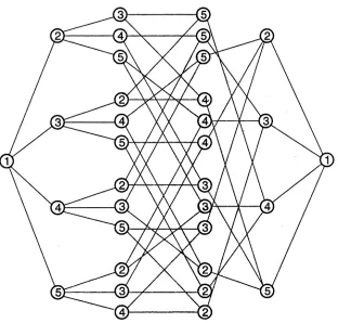
Figure 4

Illustration of the algorithm by Held and Karp for a traveling salesman problem withJ=5 cities. Not all permutations of cities have to be evaluated explicitly. For a given subset of cities the order in which the cities have been visited can be ignored.

cityj. Of all the different paths merging into the nodej, only the partial path with the smallest cost has to be retained for further computation.

3.3 DP-Based Algorithm for Statistical Machine Translation

In this section, the Held and Karp algorithm is applied to statistical MT. Using the concept of inverted alignments as introduced in Section 3.1, we explicitly take care of the coverage constraint by introducing a coverage set C of source sentence positions that have already been processed. Here, the correspondence is according to the fact that each source sentence position has to be covered exactly once, fulfilling the coverage constraint. The cities of the more complex translation TSP correspond roughly to triples

(e,e,j), the notation for which is given below. The final path output by the translation algorithm will contain exactly one triple(e,e,j)for each source positionj.

Table 2

DP-based algorithm for statistical MT that consecutively processes subsetsC of source sentence positions of increasing cardinality.

input: source language stringf1· · ·fj· · ·fJ

initialization

for each cardinalityc=1, 2,. . .,Jdo

for each pair(C,j), whereC ⊆ {1,. . .,J}andj∈ C and|C|=cdo for each pair of target wordse,e∈E

Qe(e,C,j) =p(fj|e) max

e j∈C\{j}

{p(j|j,J)·p(e|e,e)·Qe(e,C\{j},j)}

traceback:

•find best end hypothesis: max

e,e,j{p

($|e,e)·Qe(e,{1,. . .,J},j)} •recover optimal word sequence

auxiliary quantity is defined:

Qe(e,C,j) := probability of the best partial hypothesis(ei₁,bi₁), where C={bk|k=1,. . .,i},bi=j,ei=e, andei−1=e

The above auxiliary quantity satisfies the following recursive DP equation:

Qe(e,C,j) =p(f_j|e)· max

e j∈C\{j}

p(j|j,J)·p(e|e,e)·Qe(e,C\{j},j)

Here,jis the previously covered source sentence position ande,eare the predecessor words. The DP equation is evaluated recursively for each hypothesis (e,e,C,j). The resulting algorithm is depicted in Table 2. Some details concerning the initialization and the finding of the best target language string are presented in Section 3.4.p($|e,e)

is the trigram language probability for predicting the sentence boundary symbol $. The complexity of the algorithm isO(E3_·J2_·2J_{), whereEis the size of the target language}

vocabulary.

3.4 Verb Group Reordering: German to English

The above search space is still too large to translate even a medium-length input sentence. On the other hand, only very restricted reorderings are necessary; for ex-ample, for the translation direction German to English, the word order difference is mostly restricted to the German verb group. The approach presented here assumes a mostly monotonic traversal of the source sentence positions from left to right.2_{A small} number of positions may be processed sooner than they would be in that monotonic traversal. Each source position then generates a certain number of target words. The restrictions are fully formalized in Section 3.5.

A typical situation is shown in Figure 5. When translating the sentence monotoni-cally from left to right, the translation of the German finite verbkann, which is the left verbal brace in this case, is skipped until the German noun phrasemein Kollege, which is the subject of the sentence, is translated. Then, the right verbal brace is translated:

i

.

fourth

the

of

May

this

case

colleague

can

not

visit

In

e

e

F

a

k

n

n

m

i

d

I

n

s

l

l

a

m K

o

S

.

you

on

my

n

i

e

i

n

i

e

m

l

l

e

g

e

b

e

s

u

c

h

e

n

c

h

t

i

e

r

t

e

n

a v

a

M

Word reordering for the translation direction German to English: The reordering is restricted to the German verb group.

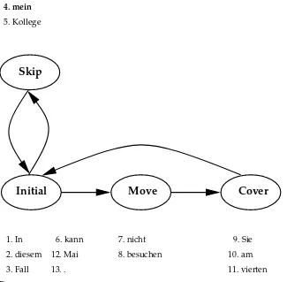
The infinitive besuchenand the negation particle nicht. The following restrictions are used: One position in the source sentence may be skipped for a distance of up toL=4 source positions, and up to two source positions may be moved for a distance of at mostR=10 source positions (the notationLandRshows the relation to the handling of the left and right verbal brace). To formalize the approach, we introduce four verb group statesS:

• Initial: A contiguous initial block of source positions is covered.

• Skip: One word may be skipped, leaving a “hole” in the monotonic traversal.

• Move: Up to two words may be “moved” from later in the sentence.

• Cover: The sentence is traversed monotonically until the stateInitial is

Initial

Skip

Move

Cover

11. vierten 5. Kollege

4. mein

1. In

3. Fall

2. diesem 12. Mai 6. kann

13. .

8. besuchen 7. nicht

10. am 9. Sie

Figure 6

Order in which the German source positions are covered for the German-to-English reordering example given in Figure 5.

The statesMoveandSkipboth allow a set of upcoming words to be processed sooner than would be the case in the monotonic traversal. The stateInitialis entered whenever there are no uncovered positions to the left of the rightmost covered position. The sequence of states needed to carry out the word reordering example in Figure 5 is given in Figure 6. The 13 source sentence words are processed in the order shown. A formal specification of the state transitions is given in Section 3.5. Any number of consecutive German verb phrases in a sentence can be processed by the algorithm. The finite-state control presented here is obtained from a simple analysis of the German-to-English word reordering problem and is not estimated from the training data. It can be viewed as an extension of the IBM-4 model distortion probabilities.

Using the above states, we define partial hypothesis extensions of the following type:

(S,C\{j},j)→(S,C,j)

lan-guage model probability p(e| $, $). Here, $ is the sentence boundary symbol, which is thought to be at position 0 in the target sentence. The search starts in the

hypoth-esis (Initial,{∅}, 0). {∅} denotes the empty set, where no source sentence position is

covered. The following recursive equation is evaluated:

Qe(e,S,C,j) (3)

=p(fj|e) max

e,S,j (S,C\{j},j)→(S,C,j)

j∈C\{j}

{p(j|j,J)·p(e|e,e)·Qe(e,S,C\{j},j)}

The search ends in the hypotheses(Initial,{1,. . .,J},j); the last covered position may be in the rangej∈ {J−L,. . .,J}, because some source positions may have been skipped at the end of the input sentence.{1,. . .,J}denotes a coverage set including all positions from position 1 to positionJ. The final translation probabilityQFis

QF= max e,e j∈{J−L,...,J}

p($|e,e)·Qe(e,Initial,{1,. . .,J},j) (4)

where p($ | e,e) denotes the trigram language model, which predicts the sentence boundary $ at the end of the target sentence.QF can be obtained using an algorithm very similar to the one given in Table 2. The complexity of the verb group reordering for the translation direction German to English is O(E3_·J·(R2_{·L·R)), as shown in} Tillmann (2001).

3.5 Word Reordering: Generalization

For the translation direction English to German, the word reordering can be restricted in a similar way as for the translation direction German to English. Again, the word order difference between the two languages is mainly due to the German verb group. During the translation process, the English verb group is decomposed as shown in Figure 7. When the sentence is translated monotonically from left to right, the trans-lation of the English finite verb canis moved, and it is translated as the German left verbal brace before the English noun phrase my colleague, which is the subject of the sentence. The translations of the infinitive visit and of the negation particle not are skipped until later in the translation process. For this translation direction, the trans-lation of one source sentence position may be moved for a distance of up to L = 4 source positions, and the translation of up to two source positions may be skipped for a distance of up to R = 10 source positions (we take over theL and R notation from the previous section). Thus, the role of the skipping and the moving are simply reversed with respect to their roles in German-to-English translation. For the example translation in Figure 7, the order in which the source sentence positions are covered is given in Figure 8.

We generalize the two approaches for the different translation directions as fol-lows: In both approaches, we assume that the source sentence is mainly processed monotonically. A small number of upcoming source sentence positions may be pro-cessed earlier than they would be in the monotonic traversal: The statesSkipandMove are used as explained in the preceding section. The positions to be processed outside the monotonic traversal are restricted as follows:

• The number of positions dealt with in the statesMove andSkip is restricted.

.

In

diesem

Fall

kann

mein

Kollege

Sie

am

vierten

Mai

nicht

besuchen

.

n h

c

o

n

o

v y

o

u

o

n

o

u

u

o M

I t

i

s

c

a

s

e

m

y

l

l

e

a

g

e

c

a

n t

i

s

i

t

t

h

e

f

t

h

r

f a

y

Word reordering for the translation direction English to German: The reordering is restricted to the English verb group.

These restrictions will be fully formalized later in this section. In the stateMove, some source sentence positions are “moved” from later in the sentence to earlier. After source sentence positions are moved, they are marked, and the translation of the sentence is continued monotonically, keeping track of the positions already covered. To formalize the approach, we introduce four reordering statesS:

• Initial: A contiguous initial block of source positions is covered.

• Skip: A restricted number of source positions may be skipped, leaving “holes” in the monotonic traversal.

• Move: A restricted number of words may be “moved” from later in the sentence.

• Cover: The sentence is traversed monotonically until the stateInitial is

reached.

To formalize the approach, the following notation is introduced: rmax(C) = max

Initial

Skip

Cover

Move

13. not

2. this 3. case 6. colleague 14. visit

15. . 4. can

5. my 7. you

8. on 9. the 10. fourth 11. of 12. May

Figure 8

Order in which the English source positions are covered for the English-to-German reordering example given in Figure 7.

lmin(C) = min

c∈C/ c

u(C) = card({c|c∈ C/ and c<rmax(C)}) m(C) = card({c|c∈ C and c>lmin(C)}) w(C) = rmax(C)−lmin(C)

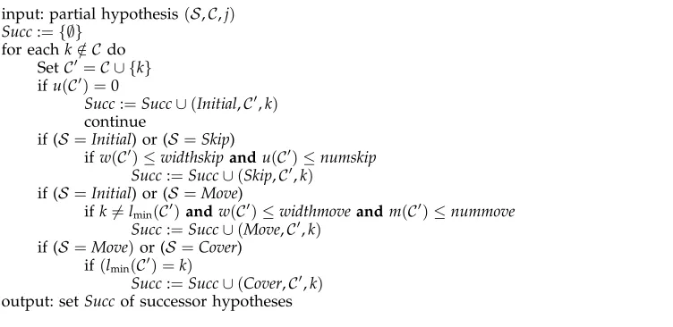
rmax(C)is the rightmost covered andlmin(C)is the leftmost uncovered source position. u(C) is the number of “skipped” positions, andm(C) is the number of “moved” po-sitions. The function card(·) returns the cardinality of a set of source positions. The functionw(C)describes the “window” size in which the word reordering takes place. A procedural description for the computation of the set of successor hypotheses for a given partial hypothesis (S,C,j) is given in Table 3. There are restrictions on the possible successor states: A partial hypothesis in state Skip cannot be expanded into a partial hypothesis in state Move and vice versa. If the coverage set for the newly generated hypothesis covers a contiguous initial block of source positions, the state

Initial is entered. No other stateSis considered as a successor state in this case (hence

Table 3

Procedural description to compute the setSuccof successor hypotheses by which to extend a partial hypothesis(S,C,j).

input: partial hypothesis(S,C,j)

Succ:={∅}

for eachk∈ C/ do SetC=C ∪ {k}

ifu(C) =0

Succ:=Succ∪(Initial,C_,k)

continue

if (S=Initial) or (S=Skip)

ifw(C)≤widthskipandu(C)≤numskip

Succ:=Succ∪(Skip,C,k)

if (S=Initial) or (S=Move)

ifk=lmin(C)andw(C)≤widthmoveandm(C)≤nummove

Succ:=Succ∪(Move,C,k)

if (S=Move)or (S=Cover)

if(lmin(C) =k)

Succ:=Succ∪(Cover,C,k)

output: setSuccof successor hypotheses

There is an asymmetry between the two reordering statesMoveandSkip: While in stateMove, the algorithm is not allowed to cover the positionlmin(C). It must first enter the stateCover to do so. In contrast, for the stateSkip, the newly generated hypothesis always remains in the stateSkip (until the stateInitial is entered.) This is motivated by the word reordering for the German verb group. After the right verbal brace has been processed, no source words may be moved into the verbal brace from later in the sentence. There is a redundancy in the reorderings: The same reordering might be carried out using either the stateSkip or Move, especially ifwidthskip and widthmove are about the same. The additional computational burden is alleviated somewhat by the fact that the pruning, as introduced in Section 3.8, does not distinguish hypotheses according to the states. A complexity analysis for different reordering constraints is given in Tillmann (2001).

3.6 Word Reordering: IBM-Style Restrictions

We now compare the new word reordering approach with the approach used in Berger et al. (1996). In the approach presented in this article, source sentence words are aligned with hypothesized target sentence words.3_{When a source sentence word is aligned, we} say its position is covered. During the search process, a partial hypothesis is extended by choosing an uncovered source sentence position, and this choice is restricted. Only one of the first n uncovered positions in a coverage set may be chosen, where n is set to 4. This choice is illustrated in Figure 9. In the figure, covered positions are marked by a filled circle, and uncovered positions are marked by an unfilled circle. Positions that may be covered next are marked by an unfilled square. The restrictions for a coverage setC can be expressed in terms of the expression u(C)defined in the previous section: The number of uncovered source sentence positions to the left of the rightmost covered position. Demanding u(C) ≤ 3, we obtain the S3 restriction

uncovered position for extension covered position

uncovered position

J

1

j

Figure 9

Illustration of the IBM-style reordering constraint.

introduced in the Appendix. An upper bound of O(E3_·J4_{) for the word reordering} complexity is given in Tillmann (2001).

3.7 Empirical Complexity Calculations

In order to demonstrate the complexity of the proposed reordering constraints, we have modified our translation algorithm to show, for the different reordering con-straints, the overall number of successor states generated by the algorithm given in Table 3. The number of successors shown in Figure 10 is counted for a pseudotransla-tion task in which a pseudo–source word xis translated into the identically pseudo– target word x. No actual optimization is carried out; the total number of successors is simply counted as the algorithm proceeds through subsets of increasing cardinality. The complexity differences for the different reordering constraints result from the dif-ferent number of coverage subsetsC and corresponding reordering states S allowed. For the different reordering constraints we obtain the following results (the abbrevia-tions MON, GE, EG, and S3 are taken from the Appendix):

• MON: For this reordering restriction, a partial hypothesis is always extended by the positionlmin(C), hence the number of processed arcs isJ.

• GE, EG: These two reordering constraints are very similar in terms of complexity: The number of word reorderings is heavily restricted in each. Actually, since the distance restrictions (expressed by the variables

widthskip andwidthmove) apply, the complexity is linear in the length of

the input sentenceJ.

1 10 100 1000 10000 100000 1e+06 1e+07

0 5 10 15 20 25 30 35 40 45 50 "J4" "S3" "EG" "GE" "MON"

1 10 100 1000 10000 100000 1e+06 1e+07

0 5 10 15 20 25 30 35 40 45 50 "J4" "S3" "EG" "GE" "MON"

Figure 10

Number of processed arcs for the pseudotranslation task as a function of the input sentence lengthJ(y-axis is given in log scale). The complexity for the four different reordering constraints MON, GE, EG, and S3 is given. The complexity of the S3 constraint is close toJ4_.

3.8 Beam Search Pruning Techniques

To speed up the search, a beam search strategy is used. There is a direct analogy to the data-driven search organization used in continuous-speech recognition (Ney et al. 1992). The full DP search algorithm proceeds cardinality-synchronously over subsets of source sentence positions of increasing cardinality. Using the beam search concept, the search can be focused on the most likely hypotheses. The hypotheses Qe(e,C,j)

are distinguished according to the coverage set C, with two kinds of pruning based on this coverage set:

1. Thecoveragepruning is carried out separately for each coverage setC. 2. Thecardinalitypruning is carried out jointly for all coverage setsC with

the same cardinalityc=c(C).

After the pruning is carried out, we retain for further consideration only hypothe-ses with a probability close to the maximum probability. The number of surviving hypotheses is controlled byfourkinds of thresholds:

• the coverage pruning thresholdt_C

• the coverage histogram thresholdnC

• the cardinality pruning thresholdtc • the cardinality histogram thresholdnc

this adjustment, for a source wordf at an uncovered source position, we precompute an upper bound ¯p(f)for the product of language model and lexicon probability:

¯

p(f) =max

e_,e,e{p(e|e

_{,e)·p(f |e)}}

The above optimization is carried out only over the word trigrams(e,e,e)that have actually been seen in the training data. Additionally, the observation pruning described below is applied to the possible translations e of a source wordf. The upper bound is used in the beam search concept to increase the comparability between hypotheses covering different coverage sets. Even more benefit from the upper bound¯p(f)can be expected if the distortion and the fertility probabilities are taken into account (Tillmann 2001). Using the definition of¯p(f), the following modified probabilityQ¯e(e,C,j)is used

to replace the original probability Qe(e,C,j), and all pruning is applied to the new

probability:

¯

Qe(e,C,j) =Qe(e,C,j)·

j∈_C¯

¯

p(fj)

For the translation experiments, equation (3) is recursively evaluated over subsets of source positions of equal cardinality. For reasons of brevity, we omit the state descrip-tionSin equation (3), since no separate pruning according to the statesSis carried out. The set of surviving hypotheses for each cardinalityc is referred to as the beam. The size of the beam for cardinalitycdepends on the ambiguity of the translation task for that cardinality. To fully exploit the speedup of the DP beam search, the search space is dynamically constructed as described in Tillmann, Vogel, Ney, Zubiaga, and Sawaf (1997), rather than using a static search space. To carry out the pruning, the maximum probabilities with respect to each coverage setC and cardinalitycare computed:

• Coverage pruning:Hypotheses are distinguished according to the subset of covered positionsC. The probabilityQˆ(C)is defined:

ˆ

Q(C) =max

e,e_,j

¯

Qe(e,C,j)

• Cardinality pruning:Hypotheses are distinguished according to the cardinalityc(C)of subsetsC of covered positions. The probabilityQˆ(c)is defined for all hypotheses withc(C) =c:

ˆ

Q(c) = max

C

c(C)=c

ˆ

Q(C)

The coverage pruning threshold tC and the cardinality pruning threshold tc are used

to prune active hypotheses. We call this pruningtranslation pruning. Hypotheses are pruned according to their translation probability:

¯

Qe(e,C,j) < tC·Qˆ(C) ¯

Qe(e,C,j) < tc·Qˆ(c)

coverage and the cardinality threshold are constant for different coverage sets C and cardinalities c. Together with the translation pruning, histogram pruning is carried out: The overall number N(C) of active hypotheses for the coverage set C and the overall number N(c) of active hypotheses for all subsets of a given cardinality may not exceed a given number; again, different numbers are used for coverage and cardi-nality pruning. The coverage histogram pruning is denoted bynC, and the cardinality histogram pruning is denoted bync:

N(C) > n_C

N(c) > nc

If the numbers of active hypotheses for each coverage set C and cardinality c, N(C)

and N(c), exceed the above thresholds, only the partial hypotheses with the highest translation probabilities are retained (e.g., we may use nC = 1,000 for the coverage histogram pruning).

The third type of pruning conductedobservation pruning: The number of words that may be produced by a source wordf is limited. For each source language word f the list of its possible translationseis sorted according to

p(f |e)·puni(e)

wherepuni(e)is the unigram probability of the target language worde. Only the bestno

target wordseare hypothesized during the search process (e.g., during the experiments to hypothesize, the bestno=50 words was sufficient.

3.9 Beam Search Implementation

In this section, we describe the implementation of the beam search algorithm presented in the previous sections and show how it is applied to the full set of IBM-4 model parameters.

3.9.1 Baseline DP Implementation. The implementation described here is similar to that used in beam search speech recognition systems, as presented in Ney et al. (1992). The similarities are given mainly in the following:

• The implementation is data driven. Both its time and memory requirements are strictly linear in the number of path hypotheses (disregarding the sorting steps explained in this section).

• The search procedure is developed to work most efficiently when the input sentences are processed mainly monotonically from left to right. The algorithm works cardinality-synchronously, meaning that all the hypotheses that are processed cover subsets of source sentence positions of equal cardinalityc.

• Since full search is prohibitive, we use a beam search concept, as in speech recognition. We use appropriate pruning techniques in connection with our cardinality-synchronous search procedure.

Table 4

Two-list implementation of a DP-based search algorithm for statistical MT. input: source stringf1· · ·fj· · ·fJ

initial hypothesis lists:S={($, $,{∅}, 0)} for each cardinalityc=1, 2,. . .,Jdo

Snew={∅}

for each hypothesis(e,e,C,j)∈ S, wherej∈ C and|C|=cdo

Expand(e,e,C,j)using probabilitiesp(fj|e)·p(j|j,J)·p(e|e,e)

Look up and add or update expanded hypothesis inSnew

Sort hypotheses inSnew according to translation score

Carry out cardinality pruning

Sort hypotheses inSnew according to coverage setCand translation score

Carry out coverage pruning

Bookkeeping of surviving hypotheses inSnew

S :=Snew

output: get best target word sequenceeI

1 from bookkeeping array

generated hypotheses. The search procedure processes subsets of covered source sen-tence positions of increasing cardinality. The search starts with S = {($, $,{∅}, 0)}, where $ denotes the sentence start symbol for the immediate two predecessor words and {∅} denotes the empty coverage set, in which no source position is covered yet. For the initial search state, the position last covered is set to 0. A set S of active hypotheses is expanded for each cardinalityc using lexicon model, language model, and distortion model probabilities. The newly generated hypotheses are added to the hypothesis set Snew; for hypotheses that are not distinguished according to our DP approach, only the best partial hypothesis is retained for further consideration. This so-called recombination is implemented as a set of simple lookup and update opera-tions on the set Snew of partial hypotheses. During the partial hypothesis extensions, an anticipated pruning is carried out: Hypotheses are discarded before they are con-sidered for recombination and are never added toSnew. (The anticipated pruning is not shown in Table 4. It is based on the pruning thresholds described in Section 3.8.) After the extension of all partial hypotheses inS, a pruning step is carried out for the hy-potheses in the newly generated setSnew. The pruning is based on two simple sorting steps on the list of partial hypotheses Snew. (Instead of sorting the partial hypothe-ses, we might have used hashing.) First, the partial hypotheses are sorted according to their translation scores (within the implementation, all probabilities are converted into translation scores by taking the negative logarithm −log()). Cardinality prun-ing can then be carried out simply by runnprun-ing down the list of hypotheses, startprun-ing with the maximum-probability hypothesis, and applying the cardinality thresholds. Then, the partial hypotheses are sorted a second time according to their coverage set

3.9.2 Details for IBM-4 Model. In this section, we outline how the DP-based beam search approach can be carried out using the full set of IBM-4 parameters. (More details can be found in Tillmann [2001] or in the cited papers.) First, the full set of IBM-4 parameters does not make the simplifying assumption given in Section 3.1, namely, that source and target sentences are of equal length: Either a target word e may be aligned with several source words (its fertility is greater than one) or a single source word may produce zero, one, or two target words, as described in Berger et al. (1996), or both. Zero target words are generated if f is aligned to the “null” word e0. Generating a single target word e is the regular case. Two target words (e,e) may be generated. The costs for generating the target worde are given by its fertility

φ(0|e)and the language model probability; no lexicon probability is used. During the experiments, we restrict ourselves to triples of target words(e,e,e)actually seen in the training data. This approach is used for the French-to-English translation experiments presented in this article.

Another approach for mapping a single source language word to several target language words involves preprocessing by the word-joining algorithm given in Till-mann (2001), which is similar to the approach presented in Och, TillTill-mann, and Ney (1999). Target words are joined during a training phase, and several joined target lan-guage words are dealt with as a new lexicon entry. This approach is used for the German-to-English translation experiments presented in this article.

In order to deal with the IBM-4 fertility parameters within the DP-based concept, we adopt the distinction between openandclosed hypothesesgiven in Berger et al. (1996). A hypothesis is said to be open if it is to be aligned with more source positions than it currently is (i.e., at least two). Otherwise it is called closed. The difference between open and closed is used to process the input sentence one position a time (for details see Tillmann 2001). The word reordering restrictions and the beam search pruning techniques are directly carried over to the full set of IBM-4 parameters, since they are based on restrictions on the coverage vectorsC only.

To ensure its correctness, the implementation was tested by carrying out forced alignments on 500 German-to-English training sentence pairs. In a forced alignment, the source sentencef₁J and the target sentenceeI₁are kept fixed, and a full search with-out re-ordering restrictions is carried with-out only over the unknown alignment aJ₁. The language model probability is divided out, and the resulting probability is compared to the Viterbi probability as obtained by the training procedure. For 499 training sentences the Viterbi alignment probability as obtained by the forced-alignment search was ex-actly the same as the one produced by the training procedure. In one case the forced-alignment search did obtain a better Viterbi probability than the training procedure.

4. Experimental Results

4.1 Performance Measures for Translation Experiments

To measure the performance of the translation methods, we use three types of au-tomatic and easy-to-use measures of the translation errors. Additionally, a subjective evaluation involving human judges is carried out (Niessen et al. 2000). The following evaluation criteria are employed:

• WER (word error rate):The WER is computed as the minimum number of substitution, insertion, and deletion operations that have to be

performed to convert the generated string into the reference target string. This performance criterion is widely used in speech recognition. The minimum is computed using a DP algorithm and is typically referred to aseditorLevenshteindistance.

• mWER (multireference WER):We use the Levenshtein distance between the automatic translation and several reference translations as a measure of the translation errors. For example, on the Verbmobil TEST-331 test set, an average of six reference translations per automatic translation are available. The Levenshtein distance between the automatic translation and each of the reference translations is computed, and the minimum Levenshtein distance is taken. The resulting measure, the mWER, is more robust than the WER, which takes into account only a single reference translation.

• PER (position-independent word error rate):In the case in which only a single reference translation per sentence is available, we introduce as an additional measure the position-independent word error rate (PER). This measure compares the words in the two sentenceswithouttaking the word order into account. Words in the reference translation that have no counterpart in the translated sentence are counted as substitution errors. Depending on whether the translated sentence is longer or shorter than the reference translation, the remaining words result in either insertion (if the translated sentence is longer) or deletion (if the translated sentence is shorter) errors. The PER is guaranteed to be less than or equal to the WER. The PER is more robust than the WER since it ignores translation errors due to different word order in the translated and reference sentences.

• SSER (subjective sentence error rate):For a more fine-grained evaluation of the translation results and to check the validity of the automatic

evaluation measures subjective judgments by test persons are carried out (Niessen et al. 2000). The following scale for the error count per sentence is used in these subjective evaluations:

0.0 : semantically correct and syntactically correct

· · · : · · ·

0.5 : semantically correct and syntactically wrong

· · · : · · ·

Table 5

Training and test conditions for the German-to-English Verbmobil corpus (*number of words without punctuation).

German English Training: Sentences 58,073

Words 519,523 549,921

Words* 418,979 453,632

Vocabulary: Size 7,911 4,648

Singletons 3,453 1,699

TEST-331: Sentences 331

Words 5,591 6,279

Bigram/Trigram Perplexity 84.0/68.2 49.3/38.3

TEST-147: Sentences 147

Words 1,968 2,173

Bigram/Trigram Perplexity — 34.6/28.1

4.2 Verbmobil Translation Experiments

4.2.1 The Task and the Corpus. The translation system is tested on the Verbmobil task (Wahlster 2000). In that task, the goal is the translation of spontaneous speech in face-to-face situations for an appointment scheduling domain. We carry out experiments for both translation directions: German to English and English to German. Although the Verbmobil task is still a limited-domain task, it is rather difficult in terms of vocabulary size, namely, about 5,000 words or more for each of the two languages; second, the syntactic structures of the sentences are rather unrestricted. Although the ultimate goal of the Verbmobil project is the translation of spokenlanguage, the input used for the translation experiments reported on in this article is mainly the (more or less) correct orthographic transcription of the spoken sentences. Thus, the effects of spontaneous speech are present in the corpus; the effect of speech recognition errors, however, is not covered. The corpus consists of 58,073 training pairs; its characteristics are given in Table 5. For the translation experiments, a trigram language model with a perplexity of 28.1 is used. The following two test corpora are used for the translation experiments: TEST-331: This test set consists of 331 test sentences. Only automatic evaluation is

carried out on this test corpus: The WER and the mWER are computed. For each test sentence in the source language there is a range of acceptable reference translations (six on average) provided by a human translator, who is asked to produce word-to-word translations wherever it is possi-ble. Part of the reference sentences are obtained by correcting automatic translations of the test sentences that are produced using the approach pre-sented in this article with different reordering constraints. The other part is produced from the source sentences without looking at any of their translations. The TEST-331 test set is used as held-out data for parameter optimization (for the language mode scaling factor and for the distortion model scaling factor). Furthermore, the beam search experiments in which the effect of the different pruning thresholds is demonstrated are carried out on the TEST-331 test set.

is carried out on the TEST-147 test set; the parameter values as obtained from the experiments on the TEST-331 test set are used.

4.2.2 Preprocessing Steps. To improve the translation performance the following preprocessing steps are carried out:

Categorization: We use some categorization, which consists of replacing a single word by a category. The only words that are replaced by a category label are proper nouns denoting German cities. Using the new labeled corpus, all probability models are trained anew. To produce translations in the “normal” language, the categories are translated by rule and are inserted into the target sentence.

Word joining: Target language words are joined using a method similar to the one described in Och, Tillmann, and Ney (1999). Words are joined to handle cases like the German compound noun “Zahnarzttermin” for the English “dentist’s appointment,” because a single word has to be mapped to two or more target words. The word joining is applied only to the target lan-guage words; the source lanlan-guage sentences remain unchanged. During the search process several joined target language words may be generated by a single source language word.

Manual lexicon: To account for unseen words in the test sentences and to obtain a greater number of focused translation probabilitiesp(f |e), we use a bilin-gual German-English dictionary. For each wordein the target vocabulary, we create a list of source translationsf according to this dictionary. The translation probabilitypdic(f |e)for the dictionary entry(f,e)is defined as

pdic(f |e) =

  

1 Ne if

(f,e)is in dictionary 0 otherwise

whereNe is the number of source words listed as translations of the

tar-get word e. The dictionary probability pdic(f | e) is linearly combined with the automatically trained translation probabilities paut(f | e) to ob-tain smoothed probabilitiesp(f |e):

p(f |e) = (1−λ)·pdic(f |e) +λ·paut(f |e)

For the translation experiments, the value of the interpolation parameter is fixed atλ=0.5.

4.2.3 Effect of the Scaling Factors. In speech recognition, in which Bayes’ decision rule is applied, a language model scaling factorαLM is used; a typical value isαLM ≈15. This scaling factor is employed because the language model probabilities are more reliably estimated than the acoustic probabilities. Following this use of a language model scaling factor in speech recognition, such a factor is introduced into statistical MT, too. The optimization criterion in equation (1) is modified as follows:

ˆ

eI₁=arg max

eI

1

{p(eI₁)αLM·_p(fJ

1 |eI1)}

wherep(eI

1)is the language model probability of the target language sentence. In the experiments presented here, a trigram language model is used to computep(eI

Table 6

Computing time, mWER, and SSER for three different reordering constraints on the TEST-147 test set. During the translation experiments, reordered words are not allowed to cross punctuation marks.

Reordering CPU time mWER SSER constraint [sec] [%] [%] MON 0.2 40.6 28.6 GE 5.2 33.3 21.0 S3 13.7 34.4 19.9

effect of the language model scaling factorα_LM is studied on the TEST-331 test set. A minimum mWER is obtained forα_LM =0.8, as reported in Tillmann (2001). Unlike in speech recognition, the translation model probabilities seem to be estimated as reliably as the language model probabilities in statistical MT.

A second scaling factor α_D is introduced for the distortion model probabilities p(j | j,J). A minimum mWER is obtained for αD = 0.4, as reported in Tillmann (2001). The WER and mWER on the TEST-331 test set increase significantly, if no distortion probability is used, for the caseα_D =0.0. The benefit of a distortion prob-ability scaling factor of α_D = 0.4 comes from the fact that otherwise, a low distor-tion probability might suppress long-distant word reordering that is important for German-to-English verb group reordering. The settingα_LM=0.8 andα_D=0.4 is used for all subsequent translation results (including the translation direction English to German).

4.2.4 Effect of the Word Reordering Constraints. Table 6 shows the computing time, mWER, and SSER on the TEST-147 test set as a function of three reordering constraints: MON, GE, and S3 (as discussed in the Appendix). The computing time is given in terms of central processing unit (CPU) time per sentence (on a 450 MHz Pentium III personal computer). For the SSER, it turns out that restricting the word reorder-ing such that it may not cross punctuation marks improves translation performance significantly. The average length of the sentence fragments that are separated by punc-tuation marks is rather small: 4.5 words per fragment. A coverage pruning threshold oftC =5.0 and an observation pruning ofno=50 are applied during the experiments.4

No other type of pruning is used.5

The MON constraint performs worst in terms of both mWER and SSER. The computing time is small, since no reordering is carried out. Constraints GE and S3 perform nearly identically in terms of both mWER and SSER. The GE constraint, however, works about three times as fast as the S3 constraint.

Table 7 shows example translations obtained under the three different reordering constraints. Again, the MON reordering constraint performs worst. In the second and third translation examples, the S3 word reordering constraint performs worse than the GE reordering constraint, since it cannot take the word reordering due to the German verb group properly into account. The German finite verbsbin (second example) and k¨onnten(third example) are too far away from the personal pronouns ichandSie (six

4 For the translation experiments, the negative logarithm of the actual pruning thresholdstcandtC is

reported; for simplicity reasons we do not change the notation.

Table 7

Example translations for the translation direction German to English using three different reordering constraints: MON, GE, and S3.

Input: Ja, wunderbar. K ¨onnen wir machen. MON: Yes, wonderful. Can we do.

GE: Yes, wonderful. We can do that. S3: Yes, wonderful. We can do that.

Input: Das ist zu knapp , weil ich ab dem dritten in Kaiserslautern bin. Genaugenommen nur am dritten.

Wie w¨are es denn am ¨ahm Samstag, dem zehnten Februar? MON: That is too tight , because I from the third in Kaiserslautern.

In fact only on the third. How about ¨ahm Saturday , the tenth of February?

GE: That is too tight, because I am from the third in Kaiserslautern. In fact only on the third.Ahm how about Saturday, February¨ the tenth?

S3: That is too tight, from the third because I will be in Kaiserslautern. In fact only on the third.Ahm how¨ about Saturday, February the tenth?

Input: Wenn Sie dann noch den siebzehnten k ¨onnten, w¨are das toll, ja. MON: If you then also the seventeenth could, would be the great, yes. GE: If you could then also the seventeenth, that would be great, yes. S3: Then if you could even take seventeenth, that would be great, yes. Input: Ja, das kommt mir sehr gelegen. Machen wir es dann

am besten so.

MON: Yes, that suits me perfectly. Do we should best like that. GE: Yes, that suits me fine. We do it like that then best. S3: Yes, that suits me fine. We should best do it like that.

and five source sentence positions, respectively) to be reordered properly. In the last example, the less restrictive S3 reordering constraint leads to a better translation; the GE translation is still acceptable, though.

4.2.5 Effect of the Beam Search Pruning Thresholds. In this section, the effect of the beam search pruning is demonstrated. Translation results on the TEST-331 test set are presented to evaluate the effectiveness of the pruning techniques.6 _{The quality of the} search algorithm with respect to the GE and S3 reordering constraints is evaluated using two criteria:

1. The number of search errors for a certain combination of pruning thresholds is counted. A search error occurs for a test sentence if the final translation probabilityQF for a candidate translationeI1 as given in equation (4) is smaller than a reference probability for that test sentence. We will compute reference probabilities two ways, as explained below. 2. The mWER performance measure is computed as a function of the

pruning thresholds used. Generally, decreasing the pruning threshold

Table 8

Effect of the coverage pruning thresholdtC on the number of search errors and mWER on the TEST-331 test set (no cardinality pruning carried out:tc=∞). A cardinality histogram pruning of 200,000 is applied to restrict the maximum overall size of the search space. The negative logarithm oftC is reported.

Reordering tC CPU time Search errors mWER constraint [sec] Qref>QF QF∗ >QF [%]

GE 0.01 0.21 318 323 73.5

0.1 0.43 231 301 53.1

1.0 1.43 10 226 30.3

2.5 4.75 5 142 25.8

5.0 29.6 — 35 24.6

7.5 156 — 2 24.9

10.0 630 — — 24.9

12.5 1300 — — 24.9

S3 0.01 5.48 314 324 70.0

0.1 9.21 225 303 50.9

1.0 46.2 4 223 31.6

2.5 190 — 129 28.4

5.0 830 — — 28.3

leads to a higher word error rate, since the optimal path through the translation lattice is missed, resulting in translation errors.

Two automatically generated reference probabilities are used. These probabilities are computed separately for the reordering constraints GE and S3 (the difference is not shown in the notation, but will be clear from the context):

Qref: A forced alignment is carried out between each of the test sentences and its corresponding reference translation; only a single reference translation for each test sentence is used. The probability obtained for the reference translation is denoted byQref.

QF∗: A translation is carried out with conservatively large pruning thresholds,

yielding a translation close to the one with the maximum translation prob-ability. The translation probability for that translation is denoted byQF∗. First, in a series of experiments we study the effect of the coverage and cardinality pruning for the reordering constraints GE and S3. (When we report on the different pruning thresholds, we will show the negative logarithm of those pruning thresholds.) The experiments are carried out on two different pruning “dimensions”:

1. In Table 8, only coverage pruning using thresholdtC is carried out; no cardinality pruning is applied:tc=∞.

2. In Table 9, only cardinality pruning using thresholdtc is carried out; no

coverage pruning is applied:t_C =∞.

Both tables use an observation pruning of no =50. The effect of the coverage

prun-ing thresholdtC is demonstrated in Table 8. For the translation experiments reported in this table, the cardinality pruning threshold is set to tc = ∞; thus, no