GA-JPDA-IMM-PF Algorithm for Tracking
Highly Maneuvering Targets
Abstract—
In this paper, we present an interesting filtering algorithm to perform accurate estimation in jump Markov nonlinear systems, in case of multi-target tracking. With this paper, we aim to contribute in solving the problem of model-based body motion estimation by using data coming from visual sensors. The Interacting Multiple Model (IMM) algorithm is specially designed to track accurately targets whose state and/or measurement (assumed to be linear) models changes during motion transition.
However, when these models are nonlinear, the IMM algorithm must be modified in order to guarantee an accurate track. In order to deal with this problem, the IMM algorithm was combined with the Unscented Kalman Filter (UKF) [6]. Even if the later algorithm proved its efficacy in nonlinear model case; it presents a serious drawback in case of non Gaussian noise. To deal with this problem we propose to substitute the UKF with the Particle Filter (PF). To overcome the problem of data association, we propose the use of the JPDA approach, [12]. To reduce the computational burden of the latter technique, we choose firstly the most likely feasible events by applying a Genetic Algorithm;finally the derived algorithm from the combination of the IMM-PF algorithm and the GA-JPDA approach is noted GA-JPDA-IMM-PF.Index Terms— Estimation, Kalman filtering, Particle filtering JPDA, Genetic algorithm Multi-Target Tracking, Visual servoing, data association.
I. INTRODUCTION
his paper hope to be a contribution within the field of visual-based control of robots, especially in visual-based tracking [3]; tracking maneuvring targets, which may themselves be robots, is a complex problem, to ensure a good track when the target switches abruptly from a motion model to another is not evident. Because of the complexity and difficulty of the problem, a simple case is considered. The study is restricted to 2-D motions of a point, whose position is given at sampling instants in terms of its Cartesian coordinates. This point may be the center of gravity of the projection of an object into a camera plane, or the result of the localisation of a mobile robot moving on a planar ground.
Several of maneuvering target tracking algorithms are developed. Among them, the interacting multiple model (IMM) method based on the optimal Kalman filter, yields good performance with efficient computation especially when
the measurement and state models are linear with Gaussian noise. However, if the later are nonlinear and/or non Gaussian noise, the standard Kalman filter should be substituted, in our study we choose the Particle Filter (PF). The algorithm derived from this combination is called IMM-PF.
Email:[msdjouad
Yacine MORSLY and Mohand Saïd DJOUADI
LaboratoireRobotique &Productique,
Ecole militaire polytechnique, BP : 17 Bordj El Bahri 16111 Alger, Algérie.
i,ymorsly]@yahoo.fr
The other problem treated in this paper, is about the data association. Effectively, at each sample time, the sensor (camera) present, several measures and observations, coming from different targets; the problem is how to affect each measure to the correct target, to deal with this problem we propose a method which computes assignment weights using the genetic algorithm and performs state update in a single step only. Genetic algorithm is widely used to solve complex optimization problem; unfortunately, there is no guarantee of obtaining the optimal assignment. But it does provide a set of potential solutions in the process of finding the best solution. In the proposed method the likelihood of an observation is modeled as a mixture pdf to incorporate multiple models explicitly. It allows one to track any arbitrary trajectory. To calculate assignment weights, a JPDA based approach is used along with the genetic algorithm. JPDA evaluates all feasible events of observation-to-track association and hence, computationally it is expensive. In our approach, we use all the best solutions (tuples) from all generations given by the genetic algorithm to calculate the assignment weights. These best tuples act as most likely feasible events. The number of best tuples found using the genetic algorithm is much less compared to the number of feasible events used in the JPDA.
The paper is organized as follows. In section II we describe the IMM algorithm PF based. In section III we present the genetic algorithm (GA) and than in section IV we present JPDA-IMM-PF algorithm. In section V we present and discuss the results of simulations. Finally in section VI we draw the conclusion.
II.THE IMM-PARTICLE FILTER ALGORITHM
The basic idea is to combine the IMM approach [1], with a particle filter one. In the derivation of the standard IMM filter, a merging and filtering process are defined. We adopt a regularized particle filter for this filtering step, and perform the merging step on the probability densities, represented by a Gaussian mixture. One consequence of the discrete nature of the approximation of the a posteriori density is that it cannot directly be applied to an IMM framework as it is used in [1].
To obtain a good continuous approximation of the a posteriori density, we use a regularized version of the bootstrap filter as first reported in [8,9]for tracking targets in clutter. In this hybrid version of the bootstrap filter, the probability density function, that has been computed as a point mass probability density on a number of grid points in the state space, is fitted to a continuous probability density function that is a sum of a prefixed number of Gaussian
density functions. Moreover, by using a hybrid type of sampling filter as an alternative for direct resampling, degeneracy in the effective number of particles is avoided [8,9]. The main advantages of the new method that we propose here are:
9 the method is able to deal with nonlinearities and non-Gaussian noise in a mode;
9 the method uses a fixed number of particles in each mode, independent of the mode probability.
Algorithm
Let a system be described by the equations:
(7) )] ( , [ )] ( , ), ( x [ h ) ( z )] ( , 1 [ w )] ( , 1 ), 1 ( x [ f ) ( x k M k v k M k k k k M k k M k k k + = − + − − =
The process noise and the measurement noise are possibly mode-dependent. Their densities are denoted by: dw[k,M(k)](w) and dν[k,M(k)](ν).
Where M(k) denotes the model at time k. It’s a finite state Markov process tacking values in
{ }
1 r j j M
= , according to a Markov transition probability matrix p assumed to be known. The probability density of the initial state is known, x(0) ∼ P0(x). Define the information up to and including time step k
as:
( )
k{
z( )
z( )
k}
Z = 1 ,...,
The filtering problem that has to be solved is:
Given a realization of Z(k) associated with (7) compute p(x(k)|Z(k)); i.e. the conditional probability density of the state x(k) given the set of measurements Z(k).
A cycle of the IMM algorithm could be summarized in four steps:
9 Interaction stage
Compute Mixing probabilities
(
−
1
−
1
)
=
1
p
(
k
−
1
c
k
k
ij ij j i
µ
µ
)
)
(8)
Compute Normalizing factors
(
∑
∈−
=
Mi ij i
j
p
k
c
µ
1
(9)
Compute A priori probability density in mode j
(
) (
)
(
)
(
)
(
)
(
1 1)
*(
1 1)
ˆ
1 1
ˆ0 0
− − − − = − −
∑
∈ k k k Z k x p k Z k x p j i M i i i j j µ (10)9 Filtering stage
M
j
∈
∀
draw N samplesx
lj(
k
−
1
)
according to(
) (
)
(
1
1
)
ˆ
0x
0k
−
Z
k
−
p
j jThe predicted samples are:
( )
k
f
(
x
(
k
k
j
)
)
w
(
k
j
)
x
l lj l
j
1
),
1
,
1
,
ˆ
=
−
−
+
−
(11)Where
w
l(
k
−
1
,
j
)
are samples obtained fromd
w(k−1,j)( )
w
The predicted output(
k
k
)
h
(
x
( )
k
k
j
)
z
lj l
j
−
1
=
ˆ
,
,
(12)The probability weight
( )
k
=
d
( ),(
z
( )
k
−
z
ˆ
(
k
k
−
1
)
)
q
lj j
k l
j ν (13)
Normalizing
( )
∑
( )
==
N l l jj
k
q
k
q
1
~
(14)Normalized probability masses
( )
( )
k
q
k
q
q
j l j lj
=
~
(15)Mean of the state over the sample set
( )
∑
( )
==
N l l j l jj
k
q
x
k
x
1
ˆ
(16)
Covariance of the state over the sample set
( )
∑
(
( )
( )
)
(
( )
( )
)
=−
−
=
N l T j l j j l j l jj
k
q
x
k
x
k
x
k
x
k
P
1
ˆ
ˆ
ˆ
(17)From the conditional probability density function for the state in mode j based on a mixture of N Gaussian densities
(
( ) ( )
)
∑
(
( )
( )
)
==
N l j j l j l j j jN
x
k
Z
k
q
N
x
k
P
k
P
1
ˆ
,
ˆ
ˆ
ν
(18)Where
ν
j=
0
.
5
N
−2dj,
and is the dimension of the state space. We obtain the probability density function for the state in mode j after mixture reduction, i.e. based on a mixture ofj
d
N
N
r≤
Gaussian densities.( ) ( )
(
)
∑
(
( )
( )
)
=
=
Nrl r j j l r j l r j j
j
x
k
Z
k
q
N
x
k
P
k
p
1 , ,ˆ
,
ˆ
ˆ
ν
(19)
The mean of predicted output over the sample set
( )
∑
(
( )
==
N l l jj
k
h
x
k
k
j
h
1
,
,
ˆ
)
(20)
Residual covariance over the sample set
( )
∑
(
(
( )
)
( )
)
(
(
( )
)
( )
)
=−
−
=
N l T j l j j l jj
k
q
h
x
k
k
j
h
k
h
x
k
k
j
h
k
Innovations
( ) ( )
k
z
k
h
(
x
l( )
k
k
j
)
j l
j
=
−
ˆ
,
,
γ
(22)Probability density function for the innovations
( ) ( )
(
k
Z
k
)
q
N
(
S
( )
k
)
N
(
S
( )
k
p
N jl
j l
j j
j
ˆ
,
0
ˆ
,
0
ˆ
1
=
=
∑
=
γ
)
(23)
Likelihoods
L
( )
k
N
(
l( )
k
S
j( )
k
)
j l
j
=
γ
;
0
,
ˆ
(24) Mode probabilities
j
( )
k
c
L
j( )
k
c
j1
=
µ
(25)Where
∑
( )
(26) ∈
=
M
j j j
c
k
L
c
9 Combination stage
The a posteriori conditional probability density function
for the stae
( ) ( )
(
)
∑
(
( ) ( )
)
( )
∈
=
M j
j j
j
x
k
Z
k
k
p
k
Z
k
x
p
ˆ
ˆ
µ
(27)IV. GENETIC ALGORITHM
Genetic algorithm and its variants have been extensively used for solving complex non-linear optimization problems [15, 16]. Genetic algorithm is based on salient operators like crossover, mutation and selection. Initially, a random set of population of elements that represent the candidate solutions is created. Crossover and mutation operations are applied on the set of population elements to generate a new set of offsprings which serve as new candidate solutions. Each element of the population of elements is assigned a fitness value (quality value) which is an indication of the performance measure. In our formulation the likelihood measure
Λ
is considered as a fitness value while designing the fitness function. In a given generation, out of the parents and the generated offsprings a set of elements are chosen based on a suitable selection mechanism. Each population of elements is represented by a string of symbols. The symbol may be either binary or real number. Each string is known as a chromosome. In our formulation, we form a string consisting of target number as a symbol. It represents a solution for data association problem i.e. observation to track (target) pairing.This string is also called as tuple. For example, with 4 measurements and 5 targets, a solution string (tuple) (2 1 4 3) indicates that observation number 1 is assigned to target 2, observation number 2 is assigned to target 1, observation number 3 is assigned to target 4, and so on. 0 in a string indicates that corresponding observation is not assigned to any
target. It may be a false alarm or a new target. If tuple is indicated by symbol n then the quality of solution is represented by function f (n), which is a fitness function. In our case, f (n) is defined as, f (n) =
∏
where i isthe observation index and t represents target number from the given tuple n. Initial population is selected from the total population space, i.e. all possible tuples. We adopt the JPDA approach which evaluates only feasible tuples, and hence the initial population consists of feasible solutions. Note that JPDA is used only for evaluating the initial population.
Λ
i
i
t
,
)
(
In our proposed method, the population size is determined dynamically. It is followed by crossover and mutation operation. These two operations are repeated for the specified number of generations or till terminating criterion is satisfied. For each generation, population set from the previous generation acts as an initial population set. The crossover operation is applied with a crossover probability. In crossover operation, two tuples are randomly chosen from the population. Then, two random indices are selected and all symbols between these two indices are swapped between two tuples selected for crossover operation. The swapping process may result in a tuple where more than one observation might be assigned to the same target and hence yields an inconsistent solution. In order to obtain a consistent solution we adopt the following crossover operation.
Let s1 and s2 be two tuples randomly chosen for crossover; next two indices p1 and p2 (p1 < p2) are randomly selected. Between these two indices all symbols between tuples s1 and
s2 are swapped. Say symbol A at index m (p1 ≤ m ≤ p2) from
s1 is to be swapped with corresponding symbol B in s2. If symbol A appears in s2 at any index other then m, say it appears at index r in s2, then symbols at index m and r in s2 are swapped. Subsequently, the symbol at m in s1 is replaced by symbol at r in s2. This process prevents the assignment of a track to multiple measurements. The above process is also applied to symbol B in s2.
Mutation operation is applied to both new solutions (tuples) obtained from the parent tuples. The mutation operation is applied with a mutation probability. In mutation operation, a random index is chosen in a tuple and it is set to mutate. First an attempt is made to mutate the observation-to-track association to the track that is unassigned in this tuple. If there is none than, it is swapped with another target number (track number) which is chosen randomly in the same tuple. After each crossover and mutation operation, these tuples are marked to indicate that the tuples are visited. This helps in the selection of two other tuples for crossover and mutation operation. Thus, all tuples are visited, and new tuples are formed. The solutions or tuples for the next generation are selected from these old and new tuples. We define the best tuple is one that has the highest fitness value defined by function f (n). It may happen that the best solution may be missed during this operation. To take care of this, the best fit tuple in a given generation is preserved for future use.
tuples from all generations are used to evaluate assignment weights. These best tuples act as most likely feasible events and now, the assignment weight (association probability) for an observation to the given target is calculated by summing over all joint events in which the marginal event of interest occurs. From simulation, it is found that number of feasible events, which are best tuples (most likely feasible events) found using the genetic algorithm, are much less compared to number of feasible events used in JPDA scheme.
V. JPDA-IMM-PFALGORITHM
The principle of the JPDA algorithm is the computation of probabilities association for each track and new measurement. These probabilities are then used as weighting coefficients in the formation of the averaged state estimate, which is used for updating each track. For a better description of the JPDA algorithm, see [2,5].
The combination of the JPDA and the IMM-PF algorithms done as follows. A single set of validated measurements for JPDA-IMM-PF is obtained by considering the intersection Zk,
of r sets of measurements corresponding to individual models:
j k r
j
k
Z
Z
1 =
=
I
Where represents the set of validated measurements under the assumption that model j is effective. The combined likelihood functions for the r modes of the IMM-PF algorithm are computed as in [6].
j k
Z
The prior mixed state estimates for model j and the validation regions for individual models are also computed as in [2,6]. The new mode probabilities, output state estimates, and corresponding error covariances are obtained as in [2,6].
VI. SIMULATIONS AND RESULTS
In this section, we perform some simulations to evaluate our algorithm (GA-JPDA-IMM-PF).
The motion models considered are the same as those presented in [4, 6]: - constant velocity on straight line (M1),
-constant acceleration on straight line (M2), - constant velocity
on circle (M3), - constant acceleration on circle (M4).
To explore the capability of our GA-JPDA-IMM-PF algorithm to track maneuvring targets, various scenarios are considered; among of them we select the typical case of three highly maneuvring targets with crossing trajectories.
We assume that the target is in a 2-D space and its position is sampled every T=1s. We run the GA-JPDA-IMM-PF with 1000 samples in each mode.
- The probability transition matrix of four models is
⎥ ⎥ ⎥ ⎥
⎦ ⎤
⎢ ⎢ ⎢ ⎢
⎣ ⎡
=
97 . 0 01 . 0 01 . 0 01 . 0
01 . 0 97 . 0 01 . 0 01 . 0
01 . 0 01 . 0 97 . 0 01 . 0
01 . 0 01 . 0 01 . 0 97 . 0
p
- The initial probability of selecting a model is 0.25, that’s to say, at the start all models have the same chance to be selected.
A. Considered scenario
We consider that we have to track simultaneously three maneuvring targets. In order to complicate the scenario, we suppose that the targets follow during there movements, crossing trajectories.
a) Target 1(blue):
The target starts moving according to model M1 until the
50th sample when an abrupt trajectory and acceleration change occur and still moving according to this during 50 samples (switching from model M1 to M4).
b) Target 2 (black):
The target starts moving according to model M1 until the
50th sample when an abrupt trajectory change occur and still moving according to this during 50 samples (switching from model M1 to M3).
c) Target 3 (green):
The target starts moving according to model M1 until the
50th sample when an abrupt acceleration about 0.2 m/s2 occur and still moving according to this during 50 samples (switching from model M1 to M2).
Fig.1. Real and Esteemed Trajectories
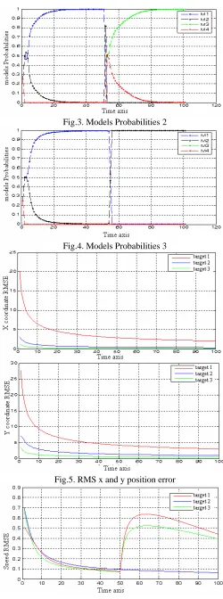
Fig.3. Models Probabilities 2
Fig.4. Models Probabilities 3
[image:5.612.317.566.52.166.2]Fig.5. RMS x and y position error
[image:5.612.316.560.60.414.2]Fig.6. RMS Acceleration and Speed Error
Fig.7. track loss rate
B. Results interpretation:
Figure 1 shows that the esteemed and the real trajectory for the three targets are superposable and almost identical even if an abrupt change occurs on the tracked target dynamic. This result is confirmed by the figures (2,3,4,5,6), from this we can say that the tracker based IMM-PF algorithm is a pertinent solution to the problem of visual-based tracking highly maneuvering targets. In the Other hand figure 2 shows also that the data association is correctly done even if the trajectories cross each other. Figure 7 shows a weak track loss rate, that is to say good performances of our algorithm. This should permit us to say that the GA-JPDA algorithm computes perfectly and its combination with the IMM-PF algorithm (GA-JPDA-IMM-PF) would be an efficient solution to the problem of highly maneuvering multi-target visual-based tracking.
VII. CONCLUSION
[image:5.612.314.564.205.337.2]REFERENCES
[1] Y.Bar-Shalom and T.E.Fortman, “Tracking and Data Association,”
Mathematics in Science and Engineering, volume 179, Academic Press,
1988.
[2] Y.Bar-Shalom and X. R. Li, “Estimation and Tracking, Principles,
Techniques and Software,” Artech House, Boston, MA (USA), 1993.
[3] B.Espiau, F.Chaumette, and P.Rives, “ A new approach to visual servoing in robotics,”IEEE Transactions on Robotics and Automation,
8(3):313-326, June 1992.
[4] P.Danes, M.S.Djouadi, D.Bellot, “A 2-D Point-Wise Motion Estimation Scheme for Visual-Based Robotic Tasks,” 7th International Symposium
on Intelligent Robotic Systems (SIRS’99), Coimbra (Portugal), 20-23
July 1999, pp.119-128
[5] Y.Bar-Shalom and X. R. Li, “Multi-target Multi-sensor Tracking:
Principles and Techniques,” Storrs, CT , YBS Publishing, 1995. [6] M.S.Djouadi, A.Sebbagh, D.Berkani, ‘‘IMM-UKF and IMM-EKF
Algorithms for Tracking Highly Maneuvring Target,’’ Archive of
Control Sciences, Vol: 1, issue: 1, 2005.
[7] M. Hadzagic, H. Mchalska, A. Jouan, " IMM-JVC and IMM-JPDA for closely maneuvering targets," IEEE, 2001.
[8] Y. Boers, JN. Driessen, " Interacting multiple model particle filter", IEE
Proc- Radar Sonar Navig, Vol.150, No. 5, October 2003.
[9] S. McGinnity, G.W. Irwin, "Multiple model bootstrap filter for maneuvering target tracking," IEEE Trans. Aerosp. Electron. Syst.,2000, 36, (3), pp. 1006–1012.
[10] S. McGinnity, G.W. Irwin, "Manoevering target tracking using a multiple-model bootstrap filter," in Doucet, A., de Freitas, N. and Gordon, N. (Eds.): ‘Sequential Monte Carlo methods in practice’ (Springer, New York, 2001), pp. 247–271
[11] N.J. Gordon,"A hybrid bootstrap filter for target tracking in clutter," IEEE Trans. Aerosp. Electron Syst., 1997, 33, (1), pp. 353–358
[12] B.Zhou, N.K. Bose, " Multitarget tracking in clutter: Fast Algorithm for Data Association," IEEE trans. Aero. Elect. Vol.29, N°.2 April 1993. [13] E.M. Reingold, J. Neivergelt, N. Deo, " Combinational Algorithms,
Theory and Practice," Prentice-Hall, 1977.
[14] T.E. Fortmann, Y. Bar-Shalom, M. Scheffe, "Sonar tracking of multiple targets using joint probabilistic data association," IEEE Journal of
Oceanic Engineering, OE-8 , July 1983.
[15] David E. Goldberg, Genetic Algorithms in Search, Optimization,
and Machine Learning, Addison-Wesley Publication,1989.
[16] K.S. Tang, K.F. Man, S. Kwong and Q. He, “Genetic Algorithms