Available online throug
ISSN 2229 – 5046
USING SQUARED-LOG ERROR LOSS FUNCTION TO ESTIMATE THE SHAPE PARAMETER
AND THE RELIABILITY FUNCTION OF PARETO TYPE I DISTRIBUTION
Huda, A. Rasheed*
Al-Mustansiriya University, Collage of Science, Dept. of Math., Iraq.
Najam A. Aleawy Al-Gazi
Math teacher at the Ministry of Eduction –Dhi Qar Iraq.
(Received on: 15-06-14; Revised & Accepted on: 16-07-14)
ABSTRACT
I
n this paper, we derived Bayes estimators for the shape parameter and the reliability function of the Pareto type I distribution under Squared-Log error loss function. In order to get better understanding of our Bayesian analysis, we consider non-informative prior for the shape parameter Using Jeffery prior Information as well as informative prior density represented by Exponential prior. According to Monte-Carlo simulation study, the performance of these estimators is compared depending on the mean square Errors (MSE’s).Key words: Pareto distribution, Reliability function, Maximum Likelihood Estimator, Bayes estimator, Squared-Log
error loss function, Jeffery prior and Exponential prior.
1. INTRODUCTION
The Pareto distribution is named after the economist Vilfredo Pareto (1848-1923), this distribution is first used as a model for the distribution of incomes a model for city population within a given area, failure model in reliability theory [1] and a queuing model in operation research [5].
A random variable X, is said to follow the two parameter Pareto distribution if its pdf is given by:
f(x;α,θ) =� θαθ
xθ+1; x≥ α ,α> 0 ,𝜃𝜃> 0 (1)
0, otherwise
where α and θ are the scale and shape parameters respectively.
The cumulative distribution function (CDF) in its simplest form is given by:
F(x;α,θ) =�1− �αx�
θ
, x≥ α; α,θ> 0
0 , otherwise (2)
So, the reliability function is:
R(t) =�αt�θ (3)
Corresponding author: Huda, A. Rasheed*
In this paper, for the simplification we’ll assume that α= 1
2. MAXIMUM LIKELIHOOD ESTIMATOR
Given x1, x2,…, xn a random sample of size n from Pareto distribution, we consider estimation using Maximum likelihood method as follows:
L(x1, … , x n|θ) =�f(xn;θ) n
i=1
L(x1, … , x n|θ) =θne−(θ+1)∑lnx
The Log- likelihood function is given by
ln L(x1, … , xn |θ) = n lnθ −(θ+ 1)�ln xi n
i=1
Differentiating the log likelihood with respect toθ: ∂[ln L(x1, … , xn|θ)]
∂θ =
n
θ − �ln xi n
i=1
Hence, the MLE of θ is: θ�ML =∑ nln x
i n i=1
θ�ML = nT , where T =�ln xi n
i=1
(4)
Using the invariant property, the MLER�ML(t) for R(t) may be obtained by replacing θ by its MLEθ�ML in (3) [6]
R�ML(t) = �1t� θ�ML
(5)
3. BAYES ESTIMATOR UNDERSQUARED-LOG ERROR LOSS FUNCTION
Bayes estimators for the shape parameter θ and Reliability function were considered under squared-log error loss function with non-Informative prior which represented by Jeffrey prior and informative loss function represented by Exponential prior where the Squared-log error loss function is of the form:
L�θ�,θ�=�lnθ� −lnθ�2
Which is balanced with 𝐿𝐿𝐿𝐿𝐿𝐿L�θ�,θ�→∞ as θ� →0 or ∞. A balanced loss function takes both error of estimation and goodness of fit into account but the unbalanced loss function only considers error of estimation. This loss function is
convex for θ�
θ ≤e and concave otherwise, but its risk function has a unique minimum with respect to θ�. [3]
According to the above mentioned loss functions, we drive the corresponding Bayes' estimators for θ using Risk function R�θ� − θ�which minimizes the posterior risk
R�θ� − θ�= E �L�θ�,θ��=� �lnθ� −lnθ�2h(θ|x1… … … . . xn)dθ ∞
0
= (lnθ�)2−2�lnθ�� E(lnθ|x) + E((lnθ)2|x)
∂Rsik
∂θ� = 2�lnθ��
1
θ�−
2
θ�E((lnθ)|x)
By letting, ∂R �θ� − θ�
∂θ� = 0
The Bayes estimator for the parameter θ of Pareto distribution under the squared-log error loss function is:
According to the Squared-Log error loss function, the corresponding Bayes' estimator for the reliability function will be:
R�(t) = Exp[E(lnR(t)|t)] (7)
E(lnR(t)|t) =�lnR(t) h(θ|t)dθ
∞
0
We have R(t) =�1
t� θ
Hence,
E[lnR(t)] = ln�1t�E[θ] (8)
Substituting (8) in (7), we get:
R�(t) = Exp�ln�1t�E[θ]� (9)
4. PRIOR AND POSTERIOR DISTRIBUTIONS
In this paper, we consider informative as well as non-informative prior density for θin order to get better understanding of our Bayesian analysis as follows:
(i) Bayes Estimator Using Jeffery Prior Information
Let us assume that θ has non-informative prior density defined by using Jeffrey prior information g1(θ) which given by:
g1(θ)∝ �I(θ)
where I(θ) represents Fisher information which defined as follows:
I(θ) =−nE�∂∂θ2lnf2�
g1(θ) = C�−nE�∂ 2lnf
∂θ2� (10)
lnf(x;θ) = lnθ −(θ+ 1)lnx
∂lnf
∂θ =
1
θ −lnx ∂2lnf
∂θ2 =−
1
θ2
E�∂∂θ2lnf2�=−θ12
After substitution in (10) we find that:
g1(θ) =θ √c n
So, the posterior distribution for θusing Jeffery prior is:
h1(θ|x) = L(x1, … , xn|θ)g1(θ)
∫0∞L(x1, … , xn|θ)g1(θ)dθ
= θ
ne−(θ+1)∑lnx c θ√n
∫ θne−(θ+1)∑lnx c θ√n dθ ∞
0
=TnθГn(n)−1e−θT (11)
θ~Gamma�n,�ln xi n
i=1
�, with:
E(θ) =∑ nln x
i n
i=1 , ver(θ) =
n (∑ni=1ln xi)2
Now,
E(lnθ|x) =ГT(n)n �∞lnθθn−1e−θTdθ 0
Let y =θT
Hence,
E(lnθ|x) =ГT(n)n �∞ln�Ty� �yT�n−1
0 e
−ydy
T =Г(n)TTn n�∞[ln y−ln T]yn−1e−ydy
0
=� ln y yГ(n)n−1e−ydy−Гln T(n)�∞yn−1
0 e
−ydy ∞
0
E(lnθ|x) =φ(n)−ln T (12) Where, φ(n) = Г(n)́
Г(n) is the digamma function [5]
Substituting (12) in (6), we get
θ�J= Exp�φ(n)−ln T� (13)
Now, using (9) to estimate Reliability function we reach to:
R
�J(t) = Exp�n
T ln� 1
t�� (14)
We can notice that R�J(t)is equivalent to the Maximum Likelihood Estimator for R(t).
(ii) Posterior Distribution Using Exponential Prior Distribution
Assuming that θ has informative prior as Exponential prior, which takes the following form:
g2(θ) =1λe−
θ
λ, θ , λ> 0
So, the posterior distribution for the parameter θ given the data (x1, x2, … xn) is:
h2�θ�X�= πi=1 n f(x
i|θ)g2(θ)
∫ π0∞ i=1 n f(xi|θ)g2(θ)dθ
Then the posterior distribution became as follows:
h2(θ|t) =
�T +1ג�n+1θne−θ�T+1ג�
Г(n + 1) (15)
This posterior density is recognized as the density of the gamma distribution
where: θ~Gamma�n + 1,1
λ+∑ni=1ln xi� , With:
E(θ) =1 n + 1
λ+∑ni=1ln xi
, ver(θ) = n + 1 (1λ+∑ni=1ln xi)
2
The Bayes estimator under Squared-Log error loss function will be:
θ�E= Exp��lnθ
∞
=�lnθ�T +
1
λ�
n+1
θne−θ�T+1λ�
Г(n + 1) dθ
∞
0
(16)
Let y =θ �T +1 λ�
Substituting in (16), we have:
E(lnθ|x) =�T +
1
λ�
n+1
Г(n + 1) �ln� y
�T +1� �
y T +1λ�
n
e−y dy
�T +1λ�
∞
0
By simplification, we get:
E(lnθ|x) =φ(n + 1) + ln�T +1λ�
θ�E= ExP�φ(n + 1) + ln�T +1λ�� (17)
Now, the corresponding Bayes estimator for R�E(t) with posterior distribution (15), come out as:
R�E(t) = ExP�
(n + 1)ln(1t)
�T +1λ� �
5. SIMULATION RESULTS
In our simulation study, we generated I = 2500 samples of sizes n = 20, 50, and100 from Pareto type I distribution to represent small, moderate and large sample size with the shape parameter θ =0.5, 1.5, 2.5 and taking t = 1.5, 3. We chose two values of λ for the Exponential prior (λ=0.5, 3).
In this section, Monte – Carlo simulation study is performed to compare the methods of estimation by using mean square Errors (MSE’s) as an index for precision to compare the efficiency of each of estimators,
where: MSE(θ�) =∑ �θ�i −θ�
2 I
i=1 I
The results were summarized and tabulated in the following tables for each estimator and for all sample sizes.
6- NUMERICAL VALUES OF ESTIMATOR (𝛉𝛉�)
The expectations and MSE’s for 𝛉𝛉are schedule in tables (1, 2, and 3) according to the sequence of tables as follows:
Table - 1: Expected Values and MSE’s of the Parameter of Pareto Distribution with θ= 0.5
θ�E
λ=3 θ�E
λ=0.5 Bayes(Jeffery)
θ�J
Criteria N
0.537547 0.513880
0.516100 Exp.(𝛉𝛉)
20
0.017743 0.013726
0.015625 MSE
0.513291 0.504564
0.504876 Exp.(𝛉𝛉)
50
0.005760 0.005226
0.005465 MSE
0.506610 0.502345
0.502409 Exp.(𝛉𝛉)
100
0.002706 0.002578
Table - 2: Expected Values and MSE’s of the Parameter of Pareto Distribution with θ= 1.5 θ�E λ=3 θ�E λ=0.5 Bayes (Jeffery) θ�J Criteria N 1.583429 1.395296 1.548297 Exp.(𝛉𝛉)
20 0.143131 0.091596 0.140624 MSE 1.529289 1.454416 1.514626 Exp.(𝛉𝛉)
50 0.049711 0.041884 0.049183 MSE 1.514685 1.477195 1.507228 Exp.(𝛉𝛉)
100
0.023851 0.021876
0.023701 MSE
Table - 3: Expected Values and MSE’s of the Parameter of Pareto Distribution with θ= 2.5
θ�E λ=3 θ�E λ=0.5 Bayes (Jeffery) θ�J Criteria N 2.592182 2.125352 2.580500 Exp.(𝛉𝛉)
20 0.359498 0.295328 0.390623 MSE 2.531424 2.332812 2.524381 Exp.(𝛉𝛉)
50 0.132948 0.122543 0.136620 MSE 2.515959 2.414210 2.512047 Exp.(𝛉𝛉)
100 0.065016 0.062163 0.065835 MSE 7. DISCUSSION
From tables (1, 2, 3) when θ=0.5, 1.5, 2.5, the simulation results show that θ�E with λ=0.5 was the best in performance, followed by θ�J (which equivalent to R�ML(t)) for different size of samples. and we can notice that MSE's increases with
increases of λ (λ =3). Finally for all sample sizes, an obvious increase in MSE is observed with the increase of the shape parameter values.
8. NUMERICAL VALUES OF ESTIMATOR 𝐑𝐑�(𝐭𝐭)
The numerical results are schedule in tables (4, 5, 6, 7, 8, and 9) according to the sequence of tables as follows:
Table - 4: Expected Values and MSE’s of the Reliability Function of Pareto Distribution with θ= 0.5, t = 1.5, (R(t)t=1.5= 0.816497)
R
�E(t) λ=3
R�E(t)
λ=0.5 Bayes (Jeffery)
R�J(t) Criteria
n
0.801013 0.808736
0.807908 Exp.𝐑𝐑(𝐭𝐭)
20 0.001967 0.001530 0.001732 MSE 0.810787 0.813665 0.813546 Exp.𝐑𝐑(𝐭𝐭)
50 0.006373 0.000577 0.000602 MSE 0.813604 0.815011 0.814982 Exp.𝐑𝐑(𝐭𝐭)
100
0.000299 0.000284
0.000290 MSE
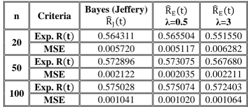
Table - 5: Expected Values and MSE’s of the Reliability Function of Pareto Distribution with θ= 0.5, t = 3, (R(t)t=3= 0.5773503)
R
�E(t) λ=3
R�E(t)
λ=0.5 Bayes (Jeffery)
R�J(t) Criteria
n
0.551550 0.565504
0.564311 Exp.𝐑𝐑(𝐭𝐭)
20 0.006282 0.005117 0.005720 MSE 0.567680 0.573075 0.572896 Exp.𝐑𝐑(𝐭𝐭)
50 0.002211 0.002035 0.002122 MSE 0.572403 0.575074 0.575028 Exp.𝐑𝐑(𝐭𝐭)
100
0.001064 0.001020
Table - 6: Expected Values and MSE’s of the Reliability Function of Pareto Distribution with θ= 1.5, t = 1.5, (R(t)t=1.5= 0.5443319)
R
�E(t) λ=3
R�E(t) λ=0.5 Bayes (Jeffery)
R�J(t)
Criteria n
0.523920 0.563970
0.531299 Exp.𝐑𝐑(𝐭𝐭)
20 0.006157 0.004498 0.006138 MSE 0.536717 0.553024 0.539809 Exp.𝐑𝐑(𝐭𝐭)
50 0.002306 0.002036 0.002299 MSE 0.540388 0.548608 0.542009 Exp.𝐑𝐑(𝐭𝐭)
100
0.001134 0.001062
0.001131 MSE
Table - 7: Expected values and MSE’s of the Reliability Function of Pareto Distribution with θ= 1.5, t = 3, (R(t)t=3= 0.1924501)
R
�E(t) λ=3
R�E(t)
λ=0.5 Bayes (Jeffery)
R�J(t)
Criteria n
0.181803 0.100107
0.188909 Exp.𝐑𝐑(𝐭𝐭)
20 0.004547 0.002969 0.004813 MSE 0.188568 0.079374 0.191610 Exp.𝐑𝐑(𝐭𝐭)
50 0.001931 0.000888 0.001980 MSE 0.190364 0.071787 0.191916 Exp.𝐑𝐑(𝐭𝐭)
100
0.000991 0.000380
0.001003 MSE
Table - 8: Expected Values and MSE’s of the Reliability Function of Pareto Distribution with θ= 2.5 , t = 1.5, (R(t)t=1.5= 0.3628883)
R
�E(t) λ=3
R�E(t)
λ=0.5 Bayes (Jeffery)
R�J(t)
Criteria n
0.350530 0.419037
0.352656 Exp.𝐑𝐑(𝐭𝐭)
20 0.006452 0.007480 0.006952 MSE 0.358448 0.387663 0.359528 Exp.𝐑𝐑(𝐭𝐭)
50 0.002661 0.002868 0.002742 MSE 0.360505 0.375469 0.361080 Exp.𝐑𝐑(𝐭𝐭)
100
0.001351 0.001400
0.001371 MSE
Table - 9: Expected Values and MSE’s of the Reliability Function of Pareto Distribution with θ= 2.5, t = 3, (R(t)t=3= 0.0071278)
R
�E(t) λ=3
R�E(t)
λ=0.5 Bayes (Jeffery)
R�J(t) Criteria
n
0.065278 0.100107
0.066859 Exp.𝐑𝐑(𝐭𝐭)
20 0.001385 0.002969 0.001538 MSE 0.064983 0.079374 0.065596 Exp.𝐑𝐑(𝐭𝐭)
50 0.000594 0.000888 0.000621 MSE 0.064521 0.071787 0.064821 Exp.𝐑𝐑(𝐭𝐭)
100 0.000305 0.000380 0.000312 MSE 9. DISCUSSION
Tables (8, 9) showing that, with a large value of θ, (θ= 2.5) MSE’s is decreases with increasing of λ (λ= 3) for the Bayes estimator with exponential prior so, we can say that R�E(t) with λ=3is better than each of the estimator with Jeffery prior (MLE) and R�E(t) with λ=0.5.
In general, we conclude that in situations involving estimation of parameter Reliability function of Pareto type I distribution under Squared-Log error loss function, using exponential prior with small value of λ (λ= 0.5) is more appropriate than using Jeffery prior (or MLE) when t,θ are small relatively (t=1.5, θ= 0.5). Otherwise using exponential prior with large value of λ (λ= 3) is better than using Jeffery prior (or MLE).
REFERENCES
[1] Nadarajah, S. & Kots, S., Reliability in Pareto models, Metron, International, Journal of statistic, vol. LXI, No.2, (2003), 191-204.
[2] Podder, C.K., Comparison of Two Risk Functions Using Pareto distribution, pak. J. States. Vol. 20(3), (2004), 369 – 378.
[3] Dey, S., “Bayesian Estimation of the Parameter of the Generalized Exponential Distribution under Different Loss Functions”, Pak. J. Stat. Oper. Res., Vol.6, No.2, (2010), 163-174.
[4] Setiya, P. & Kumar, V. “BAYESIAN ESTIMATION IN PARETO TYPE-I MODEL", Journal of Reliability and Statistical Studies; ISSN (Print): 0974-8024, (Online):2229-5666 Vol. 6, Issue 2 (2013), 139-150.
[5] Shortle, J & Fischer, M., Using the Pareto distribution in queuing modeling, Submitted Journal of probability and Statistical Science, (2005), 1 – 4.
[6] Singh, S. K., Singh, U. and Kumar, D. Bayesian Estimation of the Exponentiated Gamma Parameter and Reliability Function under Asymmetric Loss Function. REVSTAT – Statistical Journal, vol. 9, no.3, (2011), 247– 260.
Source of support: Nil, Conflict of interest: None Declared