USF Scholarship: a digital repository @ Gleeson Library |
Geschke Center
Master's Theses Theses, Dissertations, Capstones and Projects
Spring 5-23-2015
Crowded Out: The Effect of Sex Ratios on the Sex
Worker Labor Market and Migration in India
Michael Dickerson
University of San Francisco, [email protected]
Follow this and additional works at:https://repository.usfca.edu/thes
Part of theInternational Economics Commons,Labor Economics Commons, and thePolitical Economy Commons
This Thesis is brought to you for free and open access by the Theses, Dissertations, Capstones and Projects at USF Scholarship: a digital repository @ Gleeson Library | Geschke Center. It has been accepted for inclusion in Master's Theses by an authorized administrator of USF Scholarship: a digital repository @ Gleeson Library | Geschke Center. For more information, please [email protected].
Recommended Citation
Dickerson, Michael, "Crowded Out: The Effect of Sex Ratios on the Sex Worker Labor Market and Migration in India" (2015).Master's Theses. 136.
Crowded Out: The Effect of Sex Ratios on the Sex
Worker Labor Market and Migration in India
Michael Dickerson
Masters Thesis
Department of Economics University of San Francisco
2130 Fulton St. San Francisco, CA 94117
Email: [email protected]
May 2015
Introduction:
India, like several other Asian countries suffers from extremely unbalanced sex ratios. A
2002 study found that the global natural sex ratio at birth was around 1.06 males per every
female (Grech and Ventura, 2002). As of the 2011 Indian national census there were nearly 37.3
million more men than women creating a sex ratio of 940 women for every man. This is actually
lower than the already unfavorable sex ratio of 970 women for every man that was recorded
during the 2001 census (Patel, 2014). In fact Kerala is the only state in India that currently has
more women than men living in the state. Data from the 2011 census also shows that there is a
vivid divide of sex ratios between the southern and northern states in India. The three states with
the highest female-to-male sex ratios are all southern states (Kerala, Tamil Nadu, Andhra
Pradesh), while the lowest sex ratios in the country are all northern states (Haryana, Jammu and
Kashmir, Sikkim).
India’s history of distorted sex ratios can be traced back as far as 1835 with a British
Official named James Thomason. Through speaking to villages in Uttar Pradesh in 1835
Thomason learned that the birth of a daughter was considered to be a “most serious calamity and
she was seldom allowed to live”. The British then slowly realized that it was a common
occurrence to practice infanticide with daughters, which lead to the Infanticide Act of 1870,
which formally banned infanticide in India. During the first census of India in 1871 the sex ratio
stood at 940 women to 1000 men, which coincidently enough is the exact same sex ratio taken
during the last census in 2011. This ratio shocked the British and it lead to much speculation
about what causes this gap. Theories ranging from under-reporting of women from families who
distrusted the British to higher mortality rates for women because of childbirth. One British
1981). In the 20th century the practice of self-selected abortions seemed to further slant the
already distorted sex ratios. From 1982 to 1987 Mumbai experienced a dramatic rise in the
number of sex determination clinics, from 10 to 248. What may be even more alarming is one
study, which revealed that out of 8000 abortions at six different Mumbai hospitals that were
preceded by amniocentesis, 7,999 were female fetuses (Kusum, 1993). The Indian government
has opposed the practice of female infanticide and self-selective abortion, but has hardly been
efficient or effective in dealing with the matter. In 1988 the government of Maharashtra enacted
the Maharashtra Regulation of Prenatal Diagnostic Techniques Act, which mandated that
prenatal diagnostics can only be conducted to detect genetic abnormalities (including genetic
diseases linked to sex). The act, however, was riddled with loopholes and the practice though
technically illegal, continues to this day (Kusum, 1993).
This extreme shortage of women has helped to cripple local marriage markets in India,
leaving some to resort to human trafficking. The UN Office of Drugs and Crime (UNODC) have
reported that marriage trafficking rings are growing in the northern states of Haryana, Punjab,
and Uttar Pradesh. A recent 2013 survey of 92 villages in Haryana shows that in almost 10,000
households there are 9,000 married women that had been bought and transported from poor
villages in other states. Skewed sex ratios have also been linked to an increase in violent crimes
against women ranging from spousal abuse, rape, and dowry deaths (Patel, 2014). Many states
with skewed sex ratios report instances of violence against women that is well above the national
average.
This paper will examine the effect that skewed sex ratios have on the migration of Indian
sex workers through the informal labor market. Indian districts with higher sex ratios may have
informal sex labor market. This could lead to an overcrowding effect that could push these sex
workers to seek districts with less women in order to increase their bargaining power in sex
work. Districts with fewer women have worse marriage outcomes for men, which drives them to
engage with sex workers. Alternatively there could also be a demand-pull factor from districts
with lower sex ratios, as men are more desperate for women. The greater demand for sex
workers could also increase their bargaining power, allowing them to demand safer sex or even
demand more money for sexual acts. This paper uses a data set gathered by the Population
Council of 5,444 Indian sex workers in order to determine the effect sex ratios have on the
migration of sex workers.
In order to test the role sex ratios have on migration I combine data from the Population
Council dataset with census data on various demographic characteristics of Indian districts. I
then collapse the data down into a migration flow matrix that captures the flow of sex workers
from origin districts to destination districts. I then utilize a modified gravity model of migration
where low sex ratios act as a gravitational pull that attracts the female sex workers to the
districts. Gravity models typically use population differences and distance between origin and
destination as the main variables of interest, however for the purposes of this study I use sex
ratios in place of population.
The results indicate that there is a strong signal between sex ratios and the movement of
sex workers between origin and destination districts. The results show that there does seem to be
a type of overcrowding effect where sex workers are more likely to migrant from origin districts
with higher sex ratios to districts with lower sex ratios. In addition to this there seems to be
strong evidence that shows differences between different sex worker subtypes. There seems to be
very differently to one another. High-type sex workers tend to migrate to districts that have lower
sex ratios, but also have lower rates of assault on women and higher female literacy. Low-type
sex workers are much less sensitive to variables outside of sex ratio, signifying that they may
have a lower bargaining power compared to their counterparts. Sex workers are an extremely
vulnerable population in society and are often prone to sexual abuse, physical assault, and even
human trafficking. By better understanding how sex worker labor markets, and migration
patterns work policy makers can help women by improving gender outcomes. Sex work is form
of informal labor and needs to be treated that way in order to truly understand it. By viewing sex
work without passing any moral judgment not only can we get a richer understanding of how the
market works, but also how we can help the women who are engaged in the market.
This paper is organized in the following way. First I conduct a brief literature review on
migration, labor markets and sex ratios. I then describe the data as well as the theoretical and
empirical strategies that are employed. Section 3 will show the results and interpretation, which
is then followed by concluding remarks.
1. Literature Review
The literature review will briefly focus on the relevant literature for migration, labor markets,
and sex ratios. Section 1.1 will highlight various migration models, with a particular emphasis on
gravity models of migration section, section 1.2 will examine gender roles with and responses in
various labor markets, and section 1.3 will focus on the causes and implications of low sex
ratios.
1.1
Migration
Migration has been at the forefront of economic thought since the late 19th century.
who stated that “migration appeared to go on without any definite laws”. In response Ravenstein
created his seven “laws of migration” that set down the foundation for all future migration
research. Because migration is such a complex form of human behavior there are a multitude of
various theories and models that have been formed in order to explain the phenomena. Migration
can take on two separate forms: speculative migration and contracted migration. In the former
the migrants are searching for a job in another place, while in the latter migration is driven by
already finding a job in a different place (Silvers, 1977). Modern analysis on migration focuses
on the theory of job matching or as John Hicks said, “differences in net economic advantages,
chiefly differences in wages, are the main cause of migration” (Hicks, 1932). For the sake of
brevity and clarity I will restrict this all to brief literature review to only focusing on gravity
models of migration, which my research will implicitly be testing.
The gravity model, which predates even Ravenstein, focuses on the structure of the migration
response in terms of geographic constraints of a location. Simply stated the gravity model of
migration postulates that the greater the population is in a given area then the greater is the
attractive force that this area exerts. In this sense gravity is the direct ratio of the mass, and the
inverse of the distance.
Although the ideas behind the gravity model existed since the mid 19th century, it wasn’t
applied to migration until E.C. Young in the 1920’s who theorized that origin destination flow
volumes must be related to one another as the gravity model predicts. This was further expanded
upon in the 1940’s by researches like J.Q. Stewart, G.K Zipf, and Carrothers, who also applied
the gravity model to migration. Their work was set out to determine to exactly what extent the
from physics these researchers used the Newtonian formulation of gravity to spatial human
interactions.
Newton’s law was then applied to internal migration in the 1960’s by both Lee (1966)
and Lowry (1966). The intuition behind the theory assumes that migration is directly related to
the population of the origin and the inversely related to the distance between the destinations.
The basic gravity model considers not only differences in distance and population, but also
varieties of push and pull factors. Push factors are characteristics from the place of origin that
encourage migration, like low income, high unemployment etc. Pull factors are therefore those
characteristics that attract the migrant to the place of destination. In the gravity model population
size should yield positive coefficients, while distance should yield a negative coefficient.
Greenwood (1997) found that the distance elasticity of migration seemed to be decreasing over
time. He postulated that modern communication and transportation technologies might
contribute to these changes over time.
Gravity models hold an important place in the literature, but most economists have
moved on to other models. One problem with the gravity model is that the dependent variable in
the model is meant to proxy for the probability of moving from place i to place j. However, the
denominator of the dependent variable is generally population, which is measured at the
beginning or the end of the time interval. This does not accurately portray those who are truly at
risk for migration. If the population is measured in the beginning of the interval then it will
include people who will die, who were never at risk to migrate, as well as those who emigrate
from the country who can’t be counted. If population is measured at the end of the time interval
then it will include in-migrants who are not at risk of being an out-migrant considering that they
the estimation. This will help to circumvent some of the pitfalls in the gravity model, while also
playing to its strengths as using total population can lead to a biased estimate as large cities
generally attract more migrants regardless. Areas with lower sex ratios will have a gravitational
pull effect that will attract sex workers who come from areas with higher sex ratios. As other
models have become more popular in economics fewer empirical studies have been done using
the gravity model. This paper will test the gravity model empirically to determine how will it
holds up given a new set of specifications.
1.2 Labor Markets and Sex Work
Sex work by its very nature is poses multiple problems to economists trying to
understand how it works. As most sex work is illegal there is scarce data to provide an insight
into the differences between its informal labor-market. Arthur Lewis’s seminal paper,
“Economic Development with Unlimited Supplies of Labor”, helped to model the informal labor
market by developing the concept of labor market dualism. At the core of the Lewis model the
labor market can be broken down into different sectors, which can be classified as the “formal”
and informal” sectors. The essence of labor market dualism in the Lewis model depends on the
fact that workers earn different wages depending on the sector of the economy in which they are
able to find work (Lewis 1954). More recent papers, Schultz (1961, 1962), Becker (1962, 1964),
incorporate human capital theory into labor market dualism and find that in order for dualism to
exist then different wages must be paid in the different sectors to comparable workers. The
Lewis model also postulates that for the informal sector the wage is around the subsistence wage
rate. This means that when there is significant economic growth then workers are drawn from
the informal sector and into the formal sector in order to seek high wages. Sen (1967) and
also receive a higher wage than before since labor supply has gone down. House (1984) uses the
dual labor market theory to further describe different groups of people that exist in the informal
sector. One group, labeled as the “community of the poor” are people who have just arrived in a
city and are employed in the informal sector only temporarily until they can find employment in
the formal sector (this categorization is further echoed throughout the literature, most notably
Harris and Todaro, 1973). The other group is referred to as “the intermediate sector” consists of
people who have consciously decided to remain in the informal labor market due to a particular
artisan skill that they might have. This is seen as an investment as where the other group
generally lives on subsistence. While dual labor market theory is insightful, it may not be the
best lens in which to view sex work.
In order to attempt to understand how the sex market works we first need to understand
the causes of sex segregation in the labor market. Women are segregated in the labor market into
occupational categories based on traditional gender roles, which results often time in differentials
between aggregate pay for women. The neoclassical view has several hypotheses to describe
why the labor market is segmented. One such theory is the “overcrowding” effect. Fawcett and
Edgeworth (1918 and 1922) first categorize overcrowding as “that if demand for a particular
class of labor is either destroyed or very much restricted, a ‘downward pull’ on the wages is
called into existence for the whole class”. Simply put overcrowding is the relationship between
low demand for a particular type of worker who exists within a large supply of the same type of
worker. Bergmann (1971) argues that women are restricted by various demand factors that, in
turn, limit them to a particular set of occupations. This therefore results in women receiving
lower wages then men and it also constricts the mobility of women between the different
This crowding out effect could help to explain why some women choose to enter into sex
work. Edlund and Korn (2002) observe that in many cases women enter into sex work after
being crowded out of the marriage market. They argue that marriage in an important source of
income for many women and that in the absence of such income could push women to seek
other, alternative means. The authors find that on a whole sex workers tend to be married less
than the general population, as the husbands desire a wife to be faithful. Davis (1993) and Lillard
(1995) find in sex worker populations in Asia that unmarried women are overrepresented among
sex workers. However, Shah (2008), finds evidence from Ecuador and Mexico that sex workers
are more likely to be married than non-sex workers at younger ages when the earnings premium
for sex work is at its highest.
The demand for sex workers in large part is driven by men (Edlund and Korn 2002), as
the vast majority of sex workers are female. In addition there has been evidence that supports the
notion that areas with more men then women see an increase in sex workers. Bullough (1987)
shows that urban sex work in African cities is linked to very high sex ratios. Studies on sex work
in Southeast Asia have also shown a link between high sex ratios and sex work through colonial
settlement polices, military bases, and sex tourism (e.g, O’Grady 1992; Nagaraj and Yahya 1995;
Muroi and Sasaki 1997; Lim 1998). High sex ratios may make sex work more profitable relative
to marriage under certain situations. Areas that may have large seasonal influxes of men may
also have an increase in sex workers, as transient men tend to participate more in the local sex
market than the local labor market. This paper will show that there is a relationship between sex
1.2
Sex Ratios
India has a long and troubled history of son preference has helped create the widely
unbalanced sex ratios today. In these societies sons are more desired because they have higher
wage earning capacity (especially in agrarian economies, as well helping to continue the family
line, and are often the primary recipients of inheritance (Basu, 1989). Daughters are often seen
are an economic burden to poor families, in large part due to the dowry system (Matthews,
2003). This son preference manifests itself both prenatally, usually through sex-selective
abortion, and postnatally through neglect or even abandonment (Wink 2002).
Self-selective abortion remains one of the most plausible explanations for the low sex
ratio in India. One study (Jha et al. 2006) determined that self-selective abortions helped to
account for the half a million missing female births a year in India. The authors showed that
women who already had one female child were significantly more likely to abort the fetus if it
was a female. This is corroborated by a Bhardwaj (2011) paper that found that the at-birth sex
ratio was significantly lower in areas inhabited by the economic elite. The authors found that
there was a significant difference between the numbers of males and females of second birth
order, especially when the first-born was a male compared to when it was a female. Easier access
to ultra sounds and cultural preferences helped to widen this gap, especially among the wealthy
Indian elite.
While self-selected abortions were officially banned in 1994, their impact has left a nasty
legacy on gender relations in India. There has been some empirical evidence (Hudson et al.
2002) that has shown a strong link between low sex ratios and violence against women in India
perpetrated by young, unmarried men. While strong links have been found in other studies in
China (Li, 2000), there is little evidence for causation. A recent empirical study (Bose et al.
2013) did find evidence that in areas with low sex ratios violence amongst women is higher than
in areas with a more balanced ratio. Women of poor social standings, especially those in a
Scheduled Tribe or Scheduled Caste, were more likely to be beaten by their husbands and other
relatives.
While there is strong evidence that skewed sex ratios does increase rates of violence
against women, there is also evidence that an oversupply of males actually improves female
bargaining power. Chiappori et al. (2001) constructed a collective model of intra-household
bargaining and treated sex ratios as an exogenous distribution factor, which affects the
bargaining power of women. Chiappori found that if women are scarce then their weight in the
decision process increases as they face more favorable outcomes in the marriage market. This
finding is echoed by Angrist (2002) and Bulte et al (2014) who note that areas with skewed sex
ratios where there are an oversupply of men increase female bargaining power in the marriage
market. If women face favorable sex ratios, in this instance more men than women, they will
anticipate an easier marriage market and will therefore invest less into developing independent
human capital as they can expect any income loss to be supplemented by the husband. This
theory seems to be consistent with the earlier ideas of over crowding that are presented in this
paper. Sex workers who face a labor market with more women are crowded out of the market,
and will seek areas with a more favorable sex ratio as to improve their bargaining power. This
paper will further contribute to the literature by helping to illuminate how sex ratios and labor
the matter, with most studies being qualitative in nature. By establishing a link between sex
ratios and migration this paper can help to further illuminate the murky world of sex work.
2. Data and Methodology
This section will delve into both the data used for the study as well as the empirical
strategy being used. Section 2.1 will explain the data and the variables of interest. Section 2.2
will go over the estimation strategy that is used.
2.1 Data
The main data set being used is from a 2007 survey of female sex workers in India from
the Population Council survey sponsored by the Gates Foundation. The Population Council is
an international NGO that conducts research to address several critical health and
development issues in developing countries, focusing primarily on HIV and AIDS. The
survey consisted 5,444 women living in the Indian states of Andhra Pradesh, Maharashtra,
Karnataka, and Tamil. Overall the women originated from over 100 Indian districts in both
northern and southern India. These women were chosen because they were located along
trucking corridors, which are prime locations for the spread of HIV/AIDS. The women were
also selected because of their tendency to migrate. In order to qualify to be surveyed a
women had to have recently migrated at least twice, overall the women migrated an average
of five separate times. For my main analysis the unit of observation is not at the individual
women level, but instead the origin and destination districts and the flow of migrants
between them. The reasons behind this will be covered in later sections.
Table 1 presents some key summary statistics about these women including age of entry
into sex work, education level, and the number of migrations they done since being a sex
around 17. In the 2011 Indian census on average Indian women married at the age of 22,
which means these women surveyed get married much younger. This is consistent with the
findings in the literature review as earning potential is at its greatest when sex workers are
young. The mean for age of entry into sex work of 24 might suggest that some women may
have entered into sex work after being crowed out of marriage markets. Table 1 also shows
the women in the survey represent a highly mobile subset of the sex worker population, with
many women reporting over 4 distinct times of migration while being a sex worker.
Variable Observations Mean Std. Dev. Min Max
Amount Debt 2475 29915.92 805069.5 0 1000000
Age 5444 30.038 5.844 18 62
Age Married 1836 17.883 3.700 9 35
Entry Age 5444 24.087 5.096 9 41
Number of Moves 5444 6.025 3.097 2 35
Education 5444 6.155 .98 0 14
Table 1- Basic Summary Statistics – Amount Debt is in Rupees
This mobility does lead to an inherent selection bias in the data. As mentioned before these
assume that these are highly mobile sex workers who may have different patterns of behavior
from other sex workers. Also because each sex worker has migrated there is not a counterfactual
that can be easily used. This is one of the reasons why an estimation strategy that has the district
level be the unit of observation instead of individual women.
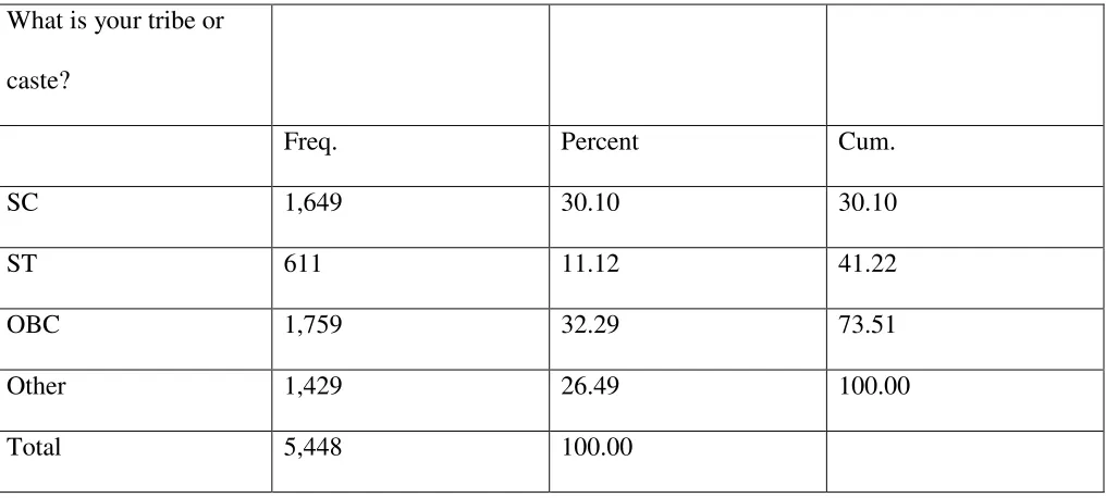
In addition to being highly mobile the women in the survey are also largely from the
Scheduled Castes and Tribes in India, as shown by Table 2. Scheduled Castes (SC) and
Scheduled Tribes (ST) are the official designation given to various ethnic groups of historically
disadvantaged people in India. The Scheduled Castes and Scheduled Tribes comprise around
16.6% and 8.6%, respectively, of India’s population at the time of the last census. In this sample
30% of the women come from a Scheduled Caste, 11.12% come from a Scheduled Tribe and
over 30% come from a “Other Backward Class” (OBC), which is another term used by the
Indian government that is used to classify a caste that is both educationally and socially
disadvantaged.
What is your tribe or
caste?
Freq. Percent Cum.
SC 1,649 30.10 30.10
ST 611 11.12 41.22
OBC 1,759 32.29 73.51
Other 1,429 26.49 100.00
Total 5,448 100.00
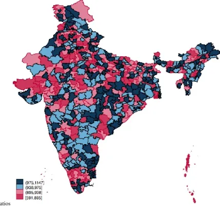
In addition to data on individual sex workers demographic and crime data from Indian
districts is also used for the estimation. Figure 1 shows a map that shows the sex ratios for each
district in India, with a darker shade indicating a higher sex ratio.
Figure 1- Map of Sex Ratios in India. Red indicates lower sex ratios, while blue indicates higher sex
ratios
The women reported 96 origin districts in the survey and they currently live in 22 districts,
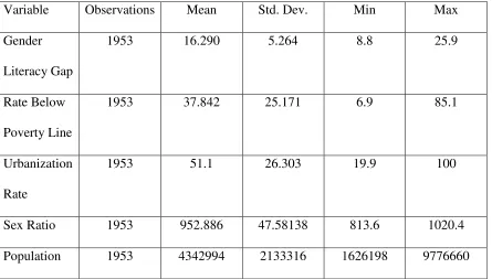
which are mostly in central and southern India. Table 3 shows various demographic data for the
origin districts reported by the women and Table 4 shows the data for destination districts
Variable Observations Mean Std. Dev. Min Max
Gender
Literacy Gap
1870 19.69 5.8777 3 30.1
Rate Below
Poverty Line
1870 47.64 23.865 6.9 95
Urbanization
Rate
1870 31.70 20.410 8.4 100
Sex Ratio 1870 963.75 42.90003 813.6 1115.2
Population 1870 3016645 1740296 552273.4 9776660
Table 3- Origin District Demographic Per Capita Summary Statistics
Variable Observations Mean Std. Dev. Min Max
Gender
Literacy Gap
1953 16.290 5.264 8.8 25.9
Rate Below
Poverty Line
1953 37.842 25.171 6.9 85.1
Urbanization
Rate
1953 51.1 26.303 19.9 100
Sex Ratio 1953 952.886 47.58138 813.6 1020.4
Population 1953 4342994 2133316 1626198 9776660
As seen in the two tables the destination district sex ratios are lower than the origin district sex
ratios, with a value of 952 and 963 respectively. As shown in the literature review sex ratios can
be seen as varying exogenously as they are dependent on a host of factors that vary different
from across districts from soil texture to self-selected abortions. However, it is reasonable to
assume that there could be other factors that are not specified that may have an effect on sex
ratios and migration. Both could be driven by economic growth or how rural a district is. This
should be taken into consideration during the estimation process. Destination districts also tend
to be more populated, less poor and have better literacy rates for women. In addition to
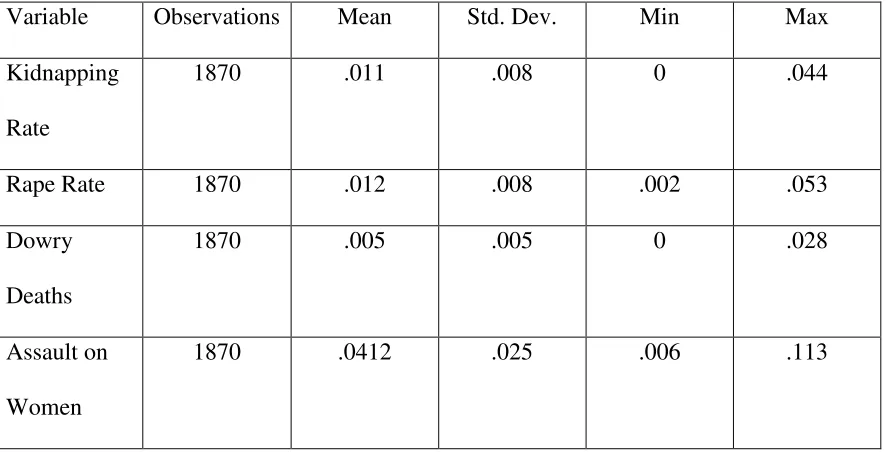
demographic data used for districts I also use various crime statistics. Sex workers are an
extremely vulnerable member of society, and are often at risk for various types of sexual and
physical violence. Tables 5 and 6 show the various crime statistics reported for origin and
destination districts respectively.
Variable Observations Mean Std. Dev. Min Max
Kidnapping
Rate
1953 .014 .010 .004 .044
Rape Rate 1953 .012 .010 .005 .053
Dowry
Deaths
1953 .004 .004 .001 .021
Assault on
Women
Table 5- Origin District Crime Stats measured in per capita values
Variable Observations Mean Std. Dev. Min Max
Kidnapping
Rate
1870 .011 .008 0 .044
Rape Rate 1870 .012 .008 .002 .053
Dowry
Deaths
1870 .005 .005 0 .028
Assault on
Women
1870 .0412 .025 .006 .113
Table 6- Destination District Crime Stats measured in per capita values.
The tables show that the differences in reported crime between the districts is relatively low.
Crime data, especially in India, is subject to reporting bias. There are incentives for some crimes
to be underreported within districts. This should be taken into consideration when this data is
used in regressions.
2.2 Empirical Strategy
One problem when using migration and spatial data is spatial autocorrelation and network
autocorrelation. Spatial autocorrelation is when variable values at given locations are influenced
by variable values at a nearby location. While network autocorrelation is concerned that the
a network context. The presence of network autocorrelation will bias any results that one may
estimate, thus proving to be a large obstacle to hurdle.
One way to tackle this problem of network autocorrelation is construct competing
destination effects and intervening opportunities. In order to do this I first collapse down all the
variables of interest by the origin and destination districts in order to get a single observation for
both the origin and destination. I then expand the dataset so that each origin district has a
potential match with a current district. This allows me to me to create a migration flow variable
where it is a 0 in counterfactual district pairs where no migrants reported moving between and
then it’s the raw number of migrants for each district where a women reported moving between.
This gives me the competing destination effects for the districts that the women did not migrate
to. By including this into the specification I can help to mitigate the effects of spatial
autocorrelation, but they may still bias any estimates that are found. I then further breakdown
migration flow into new migration flow variables of various subtypes of sex workers like those
sex workers who are highly educated compared to those sex workers who have less education.
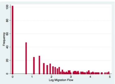
The migration flow variable is a count data where 0 means no women migrated from the
origin district to the destination district. Due to this type of data construction there is a large
abundance of 0 values for the migration flow variable, which leads to over-dispersed count data.
Count data is considered over-dispersed when the conditional variance exceeds the conditional
mean. This can be visualized by Figure 2, which shows the frequency of the migration flow
Figure 2- Over-dispersion of migration flow count data
As illustrated in Figure 2 the vast majority of the values are 0, which makes sense given the data.
Due to the over-dispersion of the data the standard OLS regression is probably not the best
estimator to use. Count outcomes are sometimes log-transformed when using OLS, which can
lead to a loss of data due to undefined values generated by taking the log of 0, which is
undefined. OLS also lacks the capacity to fully model the dispersion of the data. This means that
the most appropriate estimator to use is a negative binomial regression. Negative binomial
regressions are often used for over-dispersed data and can often be considered a generalization of
In terms of the general estimation model I follow the literature for gravity migration
models, with the one deviation of using sex ratios differentials in place for population
differentials. The model of migration flow of sex workers to districts takes the general form of
ln
Where:
= The number of women migrating from district i to district j
= The difference in sex ratios between the origin and destination district
= The measure of distance between district i to district j
= The difference between various district level controls between district i and j
= The error term
In order for this to work we must assume that there in nothing in the error term that is correlated
with both sex ratios and the migration of sex workers. Carranza (2014) finds strong evidence that
in India sex ratios have exogenous variation that stems from differences in soil textures. The
texture of soils exogenously established over millions of years as rock, minerals, and other
particles disintegrate and form the texture of the soil. Soil texture can range from very fine clay,
to loam, to very course sand. Soils that are finer have a higher particle density than coarser soils,
which makes them heavier, tighter and more difficult to work with. These soils also tend to have
very poor aeration and water intake, making them rather difficult to farm.
This varies little over time, and is extremely difficult to modify through land use. This
means that soil texture can be used as a proxy for depth of tillage, which affects the demand for
female labor. Deep tillage has been linked to demand for female labor and to the degree of
discrimination that females face. Areas with deep tillage of loamy soils tend to reduce the overall
daughters as the daughters labor becomes less and less valuable. Carranza found that the
differences between the fractions of loamy and clay soils can explain a significant portion of the
variation of child sex ratios within India.
3. Results
Regression Table 1 shows the results of my main specifications. The results seem to
indicate that sex workers do migrate to districts that have lower sex ratios. The first regression
specification shows that a one unit increase in sex ratio differences, which is the difference
between the origin district sex ratio and the destination district sex ratio, leads to an expected log
count of the number of sex workers who migrate to the current district to increase by .04. This
effect is consistent across specifications even when adding in various district level controls such
as the differences between the urbanization rates, population, and the rate of the population
below the poverty line.
The results from Regression Table 1 also provide strong evidence that lower sex ratios do
indeed attract sex workers to migrate to that district. What is particularly interesting is the signs
on the urbanization rate difference and the below poverty line rate difference. The literature on
sex workers provides strong evidence that sex workers are more likely to be clustered in poorer
areas with higher rates of urbanization. This would lead one to believe that the signs for the
variables for urbanization rate and below poverty line rate to be opposite, or that these sex
workers should also be moving to places that are more urbanized and poorer. This may be
indicating there is a crowding out effect of women that are pushing these sex workers out of their
and poorer then it would be sense that these women who are already being crowded out to avoid
districts with those characteristics.
Regression Table 1- The Effect of Sex Ratios on Migration Flow
VARIABLES Migration Flow Migration Flow Migration Flow Migration Flow
Sex Ratio Difference 0.044** 0.106*** 0.455*** 1.897*
(0.018) (0.018) (0.164) (1.117)
Distance -.001*** -.001*** -.001*** -.001***
(.004) (.004) (.004) (.004)
Below Poverty Line Rate Difference -0.388** -0.812*
(0.169) (0.445)
Urbanization Rate Difference -0.407*** -0.313*** -7.290
(0.149) (0.110) (4.753)
Population Difference -.003
(.002)
Constant -14.80*** -22.99*** 12.31 -82.27
(1.206) (3.687) (11.87) (52.35)
Observations 1,560 1,560 1,560 1,560
Origin District FE Y Y Y Y
Destination FE Y Y Y Y
Clustered standard errors in parentheses *** p<0.01, ** p<0.05, * p<0.1
Regression Table 1 Notes- Standard Errors are clustered at the origin district level. All regressions include both origin district and destination district fixed effects. Each variable is measured in the difference between the origin and destination district. Included in the Appendix are further robustness checks using a Tobit estimation.
The results from Table 1 also seem to suggest that these sex workers are engaging in a type of
investment migration. Women are migrating to districts with lower sex ratios, and therefore
better conditions for bargaining power while engaging in sex work. This also points out that a
crowding out effect is driving women to seek out better bargaining conditions. If there is
crowding out is the effect that is pushing these women to migrate to districts then is the effect
similar across different subtypes of sex workers or are there heterogeneous effects across sex
sex workers react to the same set of conditions as shown in Regression Table 1.
_______________________________________________________________________
Regression Table 2- Heterogeneous Effects of Sex Ratios and Subtype Migration Flow
Regression Table 2 Notes- Standard Errors are clustered at the origin district level. All regressions include both origin district and destination district fixed effects. Each variable is measured in the difference between the origin and destination district. Included in the Appendix are further robustness checks using a Tobit estimation. High Education sex workers are those who completed at least high school, while low education sex workers did not complete secondary school. Sex workers are considered to be in high debt if there total debt is above the mean debt of 29915 Rupees.
The results from Regression Table 2 provide an interesting insight on how different sex
worker subtypes behave. Sex workers who are more educated (for these purposes that means
having completed high school), are likelier to have high amounts of debt and be married before
entering into sex-work all respond strongly to sex ratio differentials. The first three columns,
high education sex workers, low education sex workers, and high debt sex workers, all respond
in a similar way to the regression in Table 1. Sex workers who are married, however, don’t
appear to be effected by low sex ratios. Sex workers with lower education could possibly have
VARIABLES High Education Low Education High Debt Married
Sex Ratio Diff. 2.948*** 0.129 0.176** -.003
(0.288) (0.0903) (0.075) (0.003)
Distance -.0063*** -.009*** -.009*** -.008***
(.001) (.004) (.001) (.001)
Gender Literacy Gap Diff. 0.317*** -0.102 -0.0743 -0.222**
(0.12) (0.07) (0.061) (0.095)
Below Poverty Line Rate Diff. -2.896*** -0.0592 -0.104 .018***
(0.241) (0.085) (0.07) (.005)
Urbanization Rate Diff. 1.308*** -0.265*** -0.165*** .025
(.105) (0.061) (0.057) (.007)
Constant 232.9*** -13.96* -7.309 -9.911***
(19.67) (7.298) (6.017) (1.179)
Observations 1,560 1,560 1,560 1,560
Origin District FE Y Y Y Y
Destination FE Y Y Y Y
fewer resources that would allow them to travel outside of their current district even when faced
with a crowding out effect. It is reasonable to assume that sex workers who are more educated
and sex workers who are married may have more resources at their disposal, which allows them
to respond when they are being crowded out of the labor market. These women may come from
richer families, or more urbanized districts where gender empowerment outcomes are better. Sex
workers who are more educated seem to be more responsive to labor market conditions
compared to other types of sex workers, especially the sex workers with low education. High
education sex workers seem to migrate to districts that have a more favorable sex ratio, in which
they can really take full advantage of their bargaining power, that are more urbanized, and that
have better literacy rates amongst women. These sex workers may be in a position, due to their
increased bargaining power, where they can afford to go to districts where they want to live in.
This would imply that their migration may be a form of investment, that they are migrating to
districts where may be fully utilize their human capital.
Sex workers who were in a high amount of debt when they entered into sex work seem to
respond in a fairly intuitive manner. They leave districts where they are being crowded out of the
market and they are going to less urbanized districts, places where they may not experience the
crowding out effect. Married women, on the other hand, are not very responsive to sex ratio
differentials. Married sex workers are going to poorer districts, with worse gender literacy
outcomes compared to their districts of origin. This could be due to their decreased bargaining
power within their marriage where their husbands may be the ones making the final migration
decision. Regression Table 2 indicates that there are different sex workers subtypes, “high” and
“low” types, who experience heterogeneous labor market effects. Low types seem to have less
migration as they search for better outcomes. High types on the other hand appear to be able to
migrate to districts where they would want to live in, signaling that they are engaging in an
investment migration situation.
Now that we have established how high and low type sex workers respond to various
district characteristics, I test how they respond to when migrating to the crime variables assault
on women differentials and rape differentials. Regression Table 3 shows how the sex workers
subtypes respond to these violent crimes against women.
______________________________________________________________________
Regression Table 3- Sex Worker Migration Response to Crimes Against Women
VARIABLES High Education Low Education High Debt Married
Sex Ratio Difference 0.008* 0.012*** 0.012*** 0.013***
(0.004) (0.003) (0.0023) (0.004)
Distance -0.007*** -0.009*** -0.008*** -0.008***
(0.001) (0.0004) (0.0004) (0.001)
Assault on Women Difference 16.76** 12.15** 14.55** 8.805
(8.505) (5.786) (5.898) (6.831)
Rape Difference -14.49 -0.210 6.200 -10.18
(26.97) (17.90) (17.73) (23.23)
Gender Literacy Gap Difference 0.122*** 0.136*** 0.131*** 0.121***
(0.028) (0.023) (0.023) (0.025)
Below Poverty Rate Difference -0.0374*** -0.0206*** -0.0189*** -0.0272***
(0.009) (0.007) (0.007) (0.009)
Urbanization Rate Difference 8.73e-05 0.0177*** 0.0143** 0.0161**
(0.007) (0.006) (0.006) (0.007)
Constant 1.222 1.383 1.972** 0.780
(0.915) (0.865) (0.813) (0.958)
Observations 1,560 1,560 1,560 1,560
Origin District FE Y Y Y Y
Destination FE Y Y Y Y
Robust standard errors in parentheses *** p<0.01, ** p<0.05, * p<0.1
Column one of Table 3 once again shows the migration flow sex workers who are more
educated. Consistent with the results from Table 2 these women are moving to districts that have
lower sex ratios, once again indicating an investment type migration. These women are also
going to districts that record lower indices of per capita assault against women. This is consistent
with the theory that sex worker who are better educated are seeking better economic
opportunities in other districts. These women who are faced with worse bargaining power in
their origin districts, because of crowding out in the local sex worker labor markets, are
migrating to districts where they will better economic opportunities. This could be due to a type
of beachhead effect where these women may have connections with sex workers in those
districts who are imploring them to move there, where overall economic outcomes are better due
to the lower sex ratios. Unfortunately this cannot be tests using this data set as this is one of the
limitations in the data.
Table 3 also shows that all subtypes of sex workers respond in homogeneous ways to
assault against women. Sex workers who have low education levels, high levels of debt at time
of entry and who are married are also going to districts where per capita assault against women is
lower. This once again brings up the potential of a beachhead effect that may exist in sex worker
labor markets. These women are migrating to districts that are, upon first glance, safer than their
districts of origin. The literature tells us that districts with low sex ratios are more likely to have
higher rates of assault against women, but these women are going to districts with both low sex
ratios and lower counts of per capita of assault against women. This suggests that within the sex
worker labor market information regarding safety is able to spread to sex workers of different
districts, allowing women who are more mobile to migrate to districts where they face better
4. Conclusion
The empirical results from this paper provide some much needed insight on how the
informal labor market of sex workers might work. Consistent with the previous literature, I find
strong evidence that sex workers are more likely to migrate to districts where there are fewer
women, thus giving them more bargaining power. However, it is unclear if this is due to a
crowding out effect, or a demand style pull. That sex workers in general seem to migrate to
districts that are not poorer or more urbanized indicates that this is most likely a crowding out
effect that is causing their movements. We know from the literature that sex workers tend to be
in locations that are heavily urbanized and poorer. If the women responded in a way that one
would expect given the literature then a case could be made that they are in fact moving to these
districts based off of an increase in the demand for their services.
However, it must be noted that these women are highly mobile to begin with and may not
behave in the same way as most sex workers, which significantly hampers how generalizable
these results may be. This paper also provides evidence as to how certain subtypes of sex
workers respond to similar positions. There seems to be a clear distinction between so called
“high” type and “low” type, where high type sex workers respond in a more elastic way to
changes in the labor market and they may actually engage in investment migration. This result
may also shed some more light on the murky hierarchy of the sex worker industry. It could be
that women who are highly educated may be entrepreneurial in some sense and they can make
any decision they want to regarding their work. This paper helps to contribute to the literature by
providing strong evidence that low sex ratios do cause sex workers to migrate, but whether this is
strive to include more information on the clients of sex workers, including differentials in
Appendix
Here I will go over some of the basic theory behind the gravity model. One of the
first full descriptions of the model comes from a Princeton astronomer in the 1940’s who
noticed that the distance between his student’s hometowns exhibited similar behavior to
what you could expect from the Newtonian law of gravitation. He then expressed that the
gravity law of spatial interaction looked like:
Where:
F = Gravitational or the demographic force
G = Constant
= Sex Ratio of origin
= Sex Ratio of destination
= Distance between origin and destination.
This relationship states that demographic force is directly related to the both the origin
and destination sex ratios, but it is inversely related to the distance between the two. For
the migration model M would be substituted for F in order to capture the migration flows.
In the terms of the gravity model a 1% increase in the origin or destination population
would result in a 1% increase in migration from the origin and destination as the model is
Robustness Table 1
______________________________________________________________________
Robustness Table 1- The Effect of Sex Ratios on Migration Flow
VARIABLES Tobit Tobit Tobit Tobit
Sex Ratio Difference 0.061*** 0.456*** 3.728*** 15.56***
(0.003) (0.004) (0.006) (0.005)
Distance -.056*** -.056*** -.082*** -.056***
(.0007) (.007) (.001) (.007)
Below Poverty Line Rate Difference -3.443*** -6.431***
(0.01) (0.008)
Urbanization Rate Difference -2.620*** -2.581*** -63.26***
(0.007) (0.01) (0.008)
Population Difference -0.0004***
(7.91e-08)
Constant -96.18*** -146.4*** 123.1*** -732.2***
(0.367) (0.370) (0.493) (0.375)
Observations 1,560 1,560 1,577 1,560
Origin District FE Y Y Y Y
Destination FE Y Y Y Y
Clustered standard errors in parentheses
*** p<0.01, ** p<0.05, * p<0.1
Robustness Table 2
________________________________________________________________________
Robustness Table 2- The Effect of Sex Ratios of Subtype Migration Flow
VARIABLES Tobit High Education Tobit Low Education Tobit High Debt Tobit Married
Sex Raito Difference -0.701*** 0.197*** 0.211*** 0.114***
(0.001) (0.004) (0.004) (0.003)
Distance -0.01*** -0.054*** -0.047*** -0.022***
(0.0002) (0.0007) (0.0006) (0.0004)
Urbanization Rate Difference 1.477*** -0.957*** -0.648*** -0.203***
(0.002) (0.008) (0.007) (0.004)
Gender Literacy Gap Difference -0.833*** -0.743*** -0.629*** -0.433***
(0.009) (0.03) (0.026) (0.0164)
Below Poverty Line Difference 0.835*** 0.0326*** -0.00476 0.454***
(0.002) (0.008) (0.007) (0.004)
Constant -47.24*** -105.2*** -82.94*** -62.39***
(0.103) (0.360) (0.305) (0.197)
Observations 1,560 1,560 1,560 1,560
Origin District FE Y Y Y Y
Destination FE Y Y Y Y
Clustered standard errors in parentheses
*** p<0.01, ** p<0.05, * p<0.1
Robustness Table 3
________________________________________________________________________
Robustness Table 3- Sex Worker Subtypes Response to Crimes Against Women
VARIABLES Tobit High Education Tobit Low Education Tobit High Debt Tobit Married
Sex Ratio Difference 0.959*** -0.149*** 0.0141*** -1.995***
(0.001) (0.005) (0.004) (0.003)
Distance -0.0100*** -0.0535*** -0.0466*** -0.0217***
(0.0002) (0.001) (0.001) (0.0004)
Assault on Women Difference 351.8*** 161.0*** 141.5*** -745.4***
(1.761) (6.278) (5.506) (3.146)
Rape Difference 479.8*** -2,449*** -1,890*** 433.8***
(5.725) (20.87) (18.05) (11.27)
Gender Literacy Gap Difference 0.519*** -0.484*** -0.367*** -2.388***
(0.009) (0.031) (0.027) (0.017)
Below Poverty Line Difference -0.790*** 0.0923*** -0.0297*** 2.757***
(0.002) (0.008) (0.007) (0.004)
Urbanization Rate Difference -0.419*** 0.321*** 0.267*** 1.219***
(0.002) (0.008) (0.007) (0.004)
Constant 20.55*** -69.05*** -50.36*** -183.9***
(0.102) (0.359) (0.305) (0.196)
Observations 1,560 1,560 1,560 1,560
Origin District FE Y Y Y Y
Destination FE Y Y Y Y
Clustered standard errors in parentheses
*** p<0.01, ** p<0.05, * p<0.1
References:
Arunachalam, Raj, and Manisha Shah. "ProstitutesBrides?" American Economic
Review 98.2 (2008): 516-22. Web.
Bernstein, Elizabeth. "Paying for Pleasure: Men Who Buy Sex . By
Teela Sanders . Devon: Willan Publishing, 2008. Pp. 242." American Journal of
Sociology 115.3 (2009): 909-11. Web.
Borjas, George J. "Economics of Migration." International Encyclopedia of the
Social and Behavioral Sciences, Feb. 2000. Web.
Bose, Sunita, Katherine Trent, and Scott J. South. "THE EFFECT OF A MALE
SURPLUS ON INTIMATE PARTNER VIOLENCE IN INDIA." Economic and Political
Weekly. U.S. National Library of Medicine, Aug. 2013. Web.
Bullough, Vern L. "A Nineteenth-century Transsexual." Archives of Sexual
Behavior 16.1 (1987): 81-84. Web.
Bulte, Erwin, Nico Heerink, and Xiaobo Zhang. "China's One-Child Policy and
‘the Mystery of Missing Women’: Ethnic Minorities and Male-Biased Sex
Ratios*." Oxford Bulletin of Economics and Statistics 73.1 (2011): 21-39. Web.
Bulte, Erwin, Qin Tu, and John List. "Battle of the Sexes: How Sex Ratios Affect
Female Bargaining Power." (2014): n. pag. Web.
Carranza, Eliana. "Soil Endowments, Female Labor Force Participation, and the
Demographic Deficit of Women in India." American Economic Journal: Applied
Chiapa, Carlos, and Jesus Viejo. "MIGRATION, SEX RATIOS AND VIOLENT
CRIME: EVIDENCE FROM MEXICO’S MUNICIPALITIES." Journal of Economic
Literature (n.d.): n. pag. Web. 2007.
Chun, Yongwan, Hyun Kim, and Changjoo Kim. "Modeling Interregional
Commodity Flows with Incorporating Network Autocorrelation in Spatial Interaction
Models: An Application of the US Interstate Commodity Flows." Computers,
Environment and Urban Systems 36.6 (2012): 583-91. Web.
Edlund, Lena, and Evelyn Korn. "A Theory of Prostitution." Journal of Political
Economy 110.1 (2002): 181-214. Web.
Etzo, Ivan. "Internal Migration: A Review of the Literature." Munich Personal
RePEc Archive, May 2008. Web.
Farkas, George, and Barbara R. Bergmann. "The Economic Emergence of
Women." Contemporary Sociology 16.6 (1987): 781. Web.
Fields, Gary S. "Dualism In The Labor Market: A Perspective On The Lewis
Model After Half A Century." The Manchester School 72.6 (2004): 724-35. Web.
Greenwood, Michael J., and Jesse Sexton. "On the Temporal Stability of Gravity
Models of Internal Migration." (n.d.): n. pag. Web.
Greenwood, Michael J. "Human Migration: Theory, Models, And Empirical
Studies*." Journal of Regional Science 25.4 (1985): 521-44. Web.
Greenwood, Michael J. "Migration: A Review." Regional Studies 27.4 (1993):
295-96. Web.
Gunther, Isabel, and Andrey Launov. "Competitive and Segmented Informal
Hesketh, Therese, and Zhe Wei Xing. "Abnormal Sex Ratios in Human
Populations: Causes and Consequences." Abnormal Sex Ratios in Human Populations:
Causes and Consequences. N.p., Mar. 2006. Web.
House, William J. "Nairobi's Informal Sector: Dynamic Entrepreneurs or Surplus
Labor?" Economic Development and Cultural Change 32.2 (1984): 277. Web.
Jha, P., R. Kumar, P. Vasa, N. Dhingra, D. Thiruchelvam, and R. Moineddin.
"Low Male-to-female Sex Ratio of Children Born in India: National Survey of 1·1
Million Households." The Lancet 367.9506 (2006): 211-18. Web.
Kaur, RAvinder. "Across Region Marriages: Poverty, Female Migration and the
Sex Ratio." Economic and Political Weekly 25th ser. Vol 39 (2004): n. pag. Web.
Lee, Everett S. "A Theory of Migration." Demography 3.1 (1966): 47. Web.
"Modern Gravity Models of Internal Migration. The Case of
Romania." EconPapers:. N.p., 27 Apr. 2012. Web. 04 Feb. 2015.
Murthi, Mamta, Anne-Catherine Guio, and Jean Dreze. "Mortality, Fertility, and
Gender Bias in India: A District-Level Analysis." Population and Development
Review 21.4 (1995): 745. Web.
O'grady, Kevin E. "Don Mosher." Journal of Psychology & Human Sexuality 4.4
(1992): 1-5. Web.
Patel, Archana B., Neetu Badhoniya, Manju Mamtani, and Hemant Kulkarni.
"Skewed Sex Ratios in India: “Physician, Heal Thyself”." Demography 50.3 (2013):
Rogers, Andrei, and James Raymer. "Origin Dependence, Secondary Migration,
and the Indirect Estimation of Migration Flows from Population Stocks." Journal of
Population Research22.1 (2005): 1-19. Web.
Rogers, Andrei, James Raymer, and Frans Willekens. "Capturing the Age and
Spatial Structures of Migration." Environment and Planning A 34.2 (2002): 341-59. Web.
Satchi, Mathan, and Jonathan Temple. "Labor Markets and Productivity in