Spectral Methods Meet EM: A Provably Optimal Algorithm for Crowdsourcing

Spectral Methods Meet EM: A Provably Optimal

Algorithm for Crowdsourcing

Yuchen Zhang [email protected]

Department of Electrical Engineering and Computer Science University of California, Berkeley, Berkeley, CA 94720, USA

Xi Chen [email protected]

Stern School of Business

New York University, New York, NY 10012, USA

Dengyong Zhou [email protected]

Microsoft Research

1 Microsoft Way, Redmond, WA 98052, USA

Michael I. Jordan [email protected]

Department of Electrical Engineering and Computer Science and Department of Statistics University of California, Berkeley, Berkeley, CA 94720, USA

Editor:Alexander Ihler

Abstract

Crowdsourcing is a popular paradigm for effectively collecting labels at low cost. The Dawid-Skene estimator has been widely used for inferring the true labels from the noisy labels provided by non-expert crowdsourcing workers. However, since the estimator maxi-mizes a non-convex log-likelihood function, it is hard to theoretically justify its performance. In this paper, we propose a two-stage efficient algorithm for multi-class crowd labeling prob-lems. The first stage uses the spectral method to obtain an initial estimate of parameters. Then the second stage refines the estimation by optimizing the objective function of the Dawid-Skene estimator via the EM algorithm. We show that our algorithm achieves the optimal convergence rate up to a logarithmic factor. We conduct extensive experiments on synthetic and real datasets. Experimental results demonstrate that the proposed algorithm is comparable to the most accurate empirical approach, while outperforming several other recently proposed methods.

Keywords: crowdsourcing, spectral methods, EM, Dawid-Skene model, non-convex op-timization, minimax rate

1. Introduction

For labeling tasks with k different categories, Dawid and Skene(1979) develop a max-imum likelihood approach to this problem based on the EM algorithm. They assume that each worker is associated with ak×kconfusion matrix, where the (l, c)-th entry represents the probability that a random chosen item in classlis labeled as classcby the worker. The true labels and worker confusion matrices are jointly estimated by maximizing the likelihood of the observed labels, where the unobserved true labels are treated as latent variables.

Although this EM-based approach has had empirical success (Snow et al.,2008;Raykar et al.,2010;Liu et al.,2012;Zhou et al.,2012;Chen et al.,2013;Zhou et al.,2014), there is as yet no theoretical guarantee for its performance. A recent theoretical study (Gao and Zhou, 2014) shows that the global optimal solutions of the Dawid-Skene estimator can achieve minimax rates of convergence in a simplified scenario, where the labeling task is binary and each worker has a single parameter to represent her labeling accuracy (referred to as the “one-coin” model in what follows). However, since the likelihood function is nonconvex, this guarantee is not operational because the EM algorithm can get trapped in a local optimum. Several alternative approaches have been developed that aim to circumvent the theoretical deficiencies of the EM algorithm, still the context of the one-coin model (Karger et al.,2013, 2014;Ghosh et al.,2011;Dalvi et al.,2013), but, as we survey in Section2, they either fail to achieve an optimal rate or make restrictive assumptions that can be hard to justify in practice.

We propose a computationally efficient and provably optimal algorithm to simultane-ously estimate true labels and worker confusion matrices for multi-class labeling problems. Our approach is a two-stage procedure, in which we first compute an initial estimate of worker confusion matrices using a spectral method, and then in the second stage we turn to the EM algorithm. Under some mild conditions, we show that this two-stage procedure achieves minimax rates of convergence up to a logarithmic factor, even after only one iter-ation of EM. In particular, given anyδ∈(0,1), we provide an upper bound on the number of workers and the number of items so that our method can correctly estimate labels for all items with probability at least 1−δ. We also establish a matching lower bound. Further, we provide both upper and lower bounds for estimating the confusion matrix of each worker and show that our algorithm achieves the optimal accuracy.

This work not only provides an optimal algorithm for crowdsourcing but provides new general insight into the method of moments. Empirical studies show that when the spectral method is used as an initialization for the EM algorithm, it outperforms EM with random initialization (Liang,2013;Chaganty and Liang,2013). This work provides a concrete way to justify such observations theoretically. It is also known that starting from a root-n consistent estimator obtained by the spectral method, one Newton-Raphson step leads to an asymptotically optimal estimator (Lehmann and Casella, 2003). However, obtaining a root-n consistent estimator and performing a Newton-Raphson step can be demanding computationally. In contrast, our initialization doesn’t need to be root-n consistent, thus a small portion of data suffices to initialize. Moreover, performing one iteration of EM is computationally more attractive and numerically more robust than a Newton-Raphson step especially for high-dimensional problems.

5 is devoted to theoretical analysis (with the proofs gathered in the Appendix). In Section 6, we consider the special case of the one-coin model. A simpler algorithm is introduced together with a sharper rate. Numerical results on both synthetic and real datasets are reported in Section7, followed by our conclusions in Section8.

2. Related Work

Many methods have been proposed to address the problem of estimating true labels in crowdsourcing (Whitehill et al., 2009; Raykar et al., 2010; Welinder et al., 2010; Ghosh et al.,2011;Liu et al.,2012;Zhou et al.,2012;Dalvi et al.,2013;Karger et al.,2014,2013; Parisi et al., 2014;Zhou et al., 2014). The methods in Raykar et al. (2010); Ghosh et al. (2011); Karger et al. (2014);Liu et al. (2012); Karger et al. (2013); Dalvi et al.(2013) are based on the generative model proposed byDawid and Skene (1979). In particular,Ghosh et al. (2011) propose a method based on Singular Value Decomposition (SVD) which ad-dresses binary labeling problems under the one-coin model. The analysis in Ghosh et al. (2011) assumes that the labeling matrix is full, that is, each worker labels all items. To relax this assumption,Dalvi et al. (2013) propose another SVD-based algorithm which explicitly considers the sparsity of the labeling matrix in both algorithm design and theoretical anal-ysis. Karger et al.(2014) propose an iterative algorithm for binary labeling problems under the one-coin model and extended it to multi-class labeling tasks by converting a k-class problem into k−1 binary problems (Karger et al.,2013). This line of work assumes that tasks are assigned to workers according to a random regular graph, thus imposes specific constraints on the number of workers and the number of items. In Section5, we compare our theoretical results with that of existing approaches (Ghosh et al.,2011;Dalvi et al., 2013; Karger et al., 2014, 2013). The methods in Raykar et al. (2010); Liu et al. (2012); Chen et al.(2013) incorporate Bayesian inference into the Dawid-Skene estimator by assuming a prior over confusion matrices. Zhou et al.(2012,2014) propose a minimax entropy principle for crowdsourcing which leads to an exponential family model parameterized with worker ability and item difficulty. When all items have zero difficulty, the exponential family model reduces to the generative model suggested by Dawid and Skene(1979).

Our method for initializing the EM algorithm in crowdsourcing is inspired by recent work using spectral methods to estimate latent variable models (Anandkumar et al.,2014, 2015,2012,2013;Chaganty and Liang,2013;Zou et al.,2013;Hsu et al.,2012;Jain and Oh, 2014). The basic idea in this line of work is to compute third-order empirical moments from the data and then to estimate parameters by computing a certain orthogonal decomposition of tensor derived from the moments. Given the special symmetric structure of the moments, the tensor factorization can be computed efficiently using the robust tensor power method (Anandkumar et al.,2014). A problem with this approach is that the estimation error can have a poor dependence on the condition number of the second-order moment matrix and thus empirically it sometimes performs worse than EM with multiple random initializations. Our method, by contrast, requires only a rough initialization from the moment of moments; we show that the estimation error does not depend on the condition number (see Theorem 4 (b)).

when the radius of the ball is small enough to satisfy certain gradient stability condition and sample deviation condition, EM has a geometric convergence rate. Although this is an insightful theoretical result,Balakrishnan et al. (2016) fail to provide a practical approach to constructing such an initialization.

Other related work is byDasgupta and Schulman(2007), who study an EM algorithm for learning mixture of Gaussians under certain initialization. They establish a nearly optimal estimation precision when using a two-round EM algorithm to learn the parameters from a mixture of k well-separated spherical Gaussians in the high-dimensional space. The space dimension d is assumed to be much greater than log(k). Although the high-level idea is quite similar to ours (i.e., constructing a good initializer and running one or two steps of EM), our work is different from this work in several respects. First, while Dasgupta and Schulman (2007) require the Gaussian means to be well separated, we do not assume the workers’ labeling distributions for different true labels to be separated. In fact, for any worker, we allow his/her labeling distributions for two classes to be arbitrarily close or even identical. We only assume that there is a partitioning of the workers into three groups, such that the averaged confusion matrix of each group has full rank. Second,Dasgupta and Schulman(2007) consider the high-dimensional case where the dimension of the parameter space is d log(k). In crowdsourcing, the labeling distribution lies in a k-dimensional space where k is the number of classes. Typically k is a small integer (below 10). Finally, in terms of analysis technique, Dasgupta and Schulman (2007) heavily rely on Gaussian concentration results. Our work uses a variety of techniques for different theorems. In particular, for Theorem3, we repeatedly use matrix perturbation and matrix concentration results to establish the sample complexity for the spectral method. For Theorem4, we create three random events in equation (33) (that holds with high probability), then establish both a prediction error bound and a confusion matrix estimation error bound for the EM algorithm. We use Le Cam’s method (Yu, 1997) to establish the minimax lower bound result in Theorem 5.

3. Problem Setting

Throughout this paper, [a] denotes the integer set{1,2, . . . , a} and σb(A) denotes theb-th largest singular value of matrixA. Suppose that there aremworkers,nitems andkclasses. The true labelyj of itemj ∈[n] is assumed to be sampled from a probability distribution

P[yj =l] =wl where{wl :l∈[k]} are positive values satisfyingPkl=1wl= 1. Denote by a vectorzij ∈Rk the label that workeriassigns to item j. When the assigned label is c,we

write zij =ec, where ec represents the c-th canonical basis vector in Rk in which the c-th

entry is 1 and all other entries are 0.A worker may not label every item. Letπiindicate the probability that workerilabels a randomly chosen item. If itemj is not labeled by worker i, we writezij = 0. Our goal is to estimate the true labels{yj :j∈[n]} from the observed labels{zij :i∈[m], j ∈[n]}.

Algorithm 1:Estimating confusion matrices

Input: integerk, observed labels zij ∈Rk fori∈[m] andj ∈[n]. Output: confusion matrix estimatesCb_i∈_Rk×k for i∈[m].

(1) Partition the workers into three disjoint and non-empty group G1,G2 and G3. Compute the group aggregated labels Zgj by Eq. (1).

(2) For (a, b, c)∈ {(2,3,1),(3,1,2),(1,2,3)}, compute the second and the third order moments M2c ∈_Rk×k,M3c ∈_Rk×k×k by Eq. (2a)-(2d), then computeCb_c∈_Rk×k and c

W ∈_Rk×k _{by tensor decomposition:}

(a) Compute whitening matrix Qb ∈Rk×k (such that QbTM2cQb=I) using SVD. (b) Compute eigenvalue-eigenvector pairs{(α_bh,bvh)}

k

h=1 of the whitened tensor c

M3(Q,b Q,b Qb) by using the robust tensor power method. Then compute b wh=αb

−2 h andµb

h = (QbT)−1(α_bhbvh).

(c) For l= 1, . . . , k, set thel-th column of Cb_c by some µ_bh whose l-th coordinate has the greatest component, then set thel-th diagonal entry ofWc by

b wh.

(3) ComputeCb_i by Eq. (5).

matrix of worker i. In the special case of the one-coin model, all the diagonal elements of Ci are equal to a constant while all the off-diagonal elements are equal to another constant such that each column ofCi sums to 1.

4. Our Algorithm

In this section, we present an algorithm to estimate the confusion matrices and true labels. Our algorithm consists of two stages. In the first stage, we compute an initial estimate for the confusion matrices via the method of moments. In the second stage, we perform the standard EM algorithm by taking the result of the Stage 1 as an initialization.

4.1 Stage 1: Estimating confusion matrices

Partitioning the workers into three disjoint and non-empty groups G1, G2 and G3, the outline of this stage is the following: we use the method of moments to estimate the averaged confusion matrices for the three groups, then utilize this intermediate estimate to obtain the confusion matrix of each individual worker. In particular, for g∈ {1,2,3} and j ∈[n], we calculate the averaged labeling within each group by

Zgj:= 1

|Gg| X

i∈Gg

Denoting the aggregated confusion matrix columns by

µ_gl:=E(Zgj|yj =l) = 1

|Gg| X

i∈Gg

πiµil,

our first step is to estimateC_g := [µ_g1, µ_g2, . . . , µ_gk] and to estimate the distribution of true labelsW := diag(w1, w2, . . . , wk). The following proposition shows that we can solve forCg and W from the moments of{Zgj}.

Proposition 1 (Anandkumar et al. (2015)) Assume that the vectors{µ_g1, µ_g2, . . . , µ_gk} are linearly independent for each g ∈ {1,2,3}. Let (a, b, c) be a permutation of {1,2,3}. Define

Z_aj0 :=E[Zcj⊗Zbj] (E[Zaj⊗Zbj])−1Zaj, Z_bj0 :=E[Zcj⊗Zaj] (E[Zbj⊗Zaj])−1Zbj, M2:=E[Zaj0 ⊗Z

0 bj], M3:=E[Zaj0 ⊗Zbj0 ⊗Zcj].

Then,

M2= k X

l=1

wlµcl⊗µ

cl and M3 = k X

l=1

wlµcl⊗µ cl⊗µ

cl.

Since we only have finite samples, the expectations in Proposition 1 must be approxi-mated by empirical moments. In particular, they are computed by averaging over indices j= 1,2, . . . , n. For each permutation (a, b, c)∈ {(2,3,1),(3,1,2),(1,2,3)}, we compute

b Z_aj0 :=

1 n

n X

j=1

Zcj⊗Zbj 1

n n X

j=1

Zaj⊗Zbj −1

Zaj, (2a)

b

Z_bj0 :=1 n

n X

j=1

Zcj⊗Zaj 1

n n X

j=1

Zbj⊗Zaj −1

Zbj, (2b)

c M2 :=

1 n

n X

j=1 b

Z_aj0 ⊗Zb_bj0 , (2c)

c M3 :=

1 n

n X

j=1 b

Z_aj0 ⊗Zb_bj0 ⊗Z_cj. (2d)

The statement of Proposition 1 suggests that we can recover the columns of C_c and the diagonal entries ofW by operating on the momentsM2c and M3c. This is implemented by the tensor factorization method in Algorithm 1. In particular, the tensor factorization algorithm returns a set of vectors{(µb

h,wbh) :h= 1, . . . , k}, where each (µb

It is important to note that the tensor factorization algorithm doesn’t provide a one-to-one correspondence between the recovered column and the true columns ofC_c. Thus,µb

1, . . . ,µb

k represents an arbitrary permutation of the true columns.

To discover the index correspondence, we take each _bµ_h and examine its greatest com-ponent. We assume that within each group, the probability of assigning a correct label is always greater than the probability of assigning any specific incorrect label. This as-sumption will be made precise in the next section. As a consequence, if µ_bh corresponds to the l-th column of C_c, then its l-th coordinate is expected to be greater than other coordinates. Thus, we set the l-th column of Cb_c to some vector µ_bh whose l-th coordinate has the greatest component (if there are multiple such vectors, then randomly select one of them; if there is no such vector, then randomly select a µb

h). Then, we set the l-th diagonal entry of cW to the scalar w_bh associated with µ_bh. Note that by iterating over (a, b, c) ∈ {(2,3,1),(3,1,2),(1,2,3)}, we obtain Cb_c for c = 1,2,3 respectively. There will be three copies ofWcestimating the same matrixW—we average them for the best accuracy.

In the second step, we estimate each individual confusion matrix Ci. The following proposition shows that we can recover Ci from the moments of{zij}.

Proposition 2 For any g ∈ {1,2,3} and any i ∈ Gg, let a ∈ {1,2,3}\{g} be one of the

remaining group index. Then

πiCiW(Ca)T =E[zijZajT].

Proof First, notice that

E[zijZajT] =E

E[zijZajT|yj]

= k X

l=1

wlEzijZajT|yj =l

. (3)

Since zij for 1≤i≤m are conditionally independent given yj, we can write

EzijZajT|yj =l

=E[zij|yj =l]EZajT|yj =l

= (πiµil)(µal)T. (4) Combining (3) and (4) implies the desired result,

E[zijZajT] =πi k X

l=1

wlµil(µal)T =πiCiW(Ca)T.

Proposition 2 suggests a plug-in estimator for Ci. We compute Cb_i using the empirical approximation of E[zijZajT] and using the matrices Cb_a, Cb_b, Wc obtained in the first step. Concretely, we calculate

b

Ci := normalize  

 1

n n X

j=1 zijZajT

c W(Cb_a)T

−1  



, (5)

4.2 Stage 2: EM algorithm

The second stage is devoted to refining the initial estimate provided by Stage 1. The joint likelihood of true label yj and observed labels zij, as a function of confusion matrices µi, can be written as

L(µ;y, z) := n Y

j=1 m Y

i=1 k Y

c=1 (µiyjc)

I(zij=ec)_.

By assuming a uniform prior overy, we maximize the marginal log-likelihood function

`(µ) := log 

 X

y∈[k]n

L(µ;y, z) 

. (6)

We refine the initial estimate of Stage 1 by maximizing the objective function (6), which is implemented by the Expectation Maximization (EM) algorithm. The EM algorithm takes as initialization the values {µ_bilc} provided as output by Stage 1, and then executes the following E-step and M-step for at least one round.

E-step Calculate the expected value of the log-likelihood function, with respect to the conditional distribution ofy given z under the current estimate of µ:

Q(µ) :=Ey|z,bµ[log(L(µ;y, z))] =

n X

j=1 ( _k

X

l=1 b qjllog

m Y

i=1 k Y

c=1

(µilc)I(zij=ec) !)

,

where qbjl←

exp Pm i=1

Pk

c=1I(zij =ec) log(bµilc)

Pk l0₌₁exp

Pm i=1

Pk

c=1I(zij =ec) log(µbil0c)

forj∈[n],l∈[k]. (7)

M-step Find the estimate µbthat maximizes the functionQ(µ):

b µilc←

Pn

j=1qbjlI(zij =ec) Pk

c0₌₁

Pn

j=1qbjlI(zij =ec0)

fori∈[m],l∈[k], c∈[k]. (8)

In practice, we alternatively execute the updates (7) and (8), for one iteration or until convergence. Each update increases the objective function `(µ). Since`(µ) is not concave, the EM update doesn’t guarantee converging to the global maximum. It may converge to distinct local stationary points for different initializations. Nevertheless, as we prove in the next section, it is guaranteed that the EM algorithm will output statistically optimal estimates of true labels and worker confusion matrices if it is initialized by Algorithm 1.

5. Convergence Analysis

To state our main theoretical results, we first need to introduce some notation and assump-tions. Let

be the smallest portion of true labels and the most extreme sparsity level of workers. Our first assumption assumes that both wmin and πmin are strictly positive, that is, every class

and every worker contributes to the dataset.

Our second assumption assumes that the confusion matrices for each of the three groups, namely C₁, C₂ and C₃, are nonsingular. As a consequence, if we define matrices Sab and tensors Tabc for any a, b, c∈ {1,2,3}as

Sab:= k X

l=1

wlµal⊗µ bl =C

aW(C

b)T and Tabc:= k X

l=1

wlµal⊗µ bl⊗µ

cl,

then there will be a positive scalarσL such that σk(Sab)≥σL>0.

Our third assumption assumes that within each group, the average probability of assign-ing a correct label is always higher than the average probability of assignassign-ing any incorrect label. To make this statement rigorous, we define a quantity

κ:= min

g∈{1,2,3}minl∈[k]c∈[mink]\{l}{µ gll−µ

glc}

indicating the smallest gap between diagonal entries and non-diagonal entries in the confu-sion matrix. The assumption requires thatκ is strictly positive. Note that this assumption is group-based, thus doesn’t assume the accuracy of any individual worker.

Finally, we introduce a quantity that measures the average ability of workers in

identify-ing distinct labels. For two discrete distributionsP andQ, letDKL(P, Q) :=P_iP(i) log(P(i)/Q(i)) represent the KL-divergence betweenP and Q. Since each column of the confusion matrix

represents a discrete distribution, we can define the following quantity:

D= min l6=l0

1 m

m X

i=1

πiDKL(µil, µil0). (9)

The quantity D lower bounds the averaged KL-divergence between two columns. If D is strictly positive, it means that every pair of labels can be distinguished by at least one subset of workers. As the last assumption, we assume thatD is strictly positive.

The following two theorems characterize the performance of our algorithm. We split the convergence analysis into two parts. Theorem3characterizes the performance of Algo-rithm 1, providing sufficient conditions for achieving an arbitrarily accurate initialization. We provide the proof of Theorem3 in AppendixA.

Theorem 3 For any scalar δ > 0 and any scalar satisfying ≤minn_π 36κk

minwminσL,2

o

, if the number of items nsatisfies

n= Ω

k5log((k+m)/δ) 2_π2

minwmin2 σ

13 L

,

then the confusion matrices returned by Algorithm 1 are bounded as

kCb_i−C_ik_∞≤ for all i∈[m],

Theorem 4 characterizes the error rate in Stage 2. It states that when a sufficiently accurate initialization is taken, the updates (7) and (8) refine the estimatesµb andybto the optimal accuracy. See Appendix Bfor the proof.

Theorem 4 Assume that µilc ≥ρ holds for all (i, l, c)∈[m]×[k]2. For any scalar δ >0,

if confusion matrices Cb_i are initialized in a way such that

kCb_i−C_ik∞≤α:= min

ρ 2,

ρD 16

for alli∈[m] (10)

and the number of workers m and the number of items n satisfy

m= Ω

log(1/ρ) log(kn/δ) D

and n= Ω

log(mk/δ) πminwminα2

,

then, for _bµandq_bobtained by iterating (7) and (8)(for at least one round), with probability at least 1−δ,

(a) Let y_bj = arg maxl∈[k]qbjl, then ybj =yj holds for allj∈[n].

(b) kµ_bil−µilk22 ≤

48 log(8mk/δ)

πiwln holds for all(i, l)∈[m]×[k].

In Theorem 4, the assumption that all confusion matrix entries are lower bounded by ρ >0 is somewhat restrictive. For datasets violating this assumption, we enforce positive confusion matrix entries by adding random noise: Given any observed label zij, we replace it by a random label in {1, ..., k} with probability kρ. In this modified model, every entry of the confusion matrix is lower bounded byρ, so that Theorem4holds. The random noise makes the constantD smaller than its original value, but the change is minor for smallρ.

To see the consequence of the convergence analysis, we take error rate in Theorem 3 equal to the constantα defined in Theorem4. Then we combine the statements of the two theorems. This shows that if we choose the number of workersm and the number of items nsuch that

m=Ωe

1 D

and n=Ωe

k5 π2

minw2minσ

13

L min{ρ2,(ρD)2} !

; (11)

that is, if both mand nare lower bounded by a problem-specific constant and logarithmic terms, then with high probability, the predictor _by will be perfectly accurate, and the esti-mator µ_b will be bounded as k_bµil−µilk22 ≤ Oe(1/(π_iw_ln)). To show the optimality of this convergence rate, we present the following minimax lower bounds. See AppendixCfor the proof.

(a) For any {µilc}, {πi} and any number of itemsn, if the number of workers m≤1/(4D),

then

inf

b

y _vsup_∈[k]nE

h_Xn

j=1

I(ybj 6=yj)

{µilc},{πi}, y =v i

≥c1n.

(b) For any{wl},{πi}, any worker-item pair(m, n)and any pair of indices(i, l)∈[m]×[k],

we have

inf

b

µ _µ∈sup

Rm×k×k

E h

kµ_bil−µilk22

{wl},{πi} i

≥c2 min

1, 1 πiwln

.

In part (a) of Theorem 5, we see that the number of workers should be at least 1/D, otherwise any predictor will make many mistakes. This lower bound matches our sufficient condition on the number of workers m (see Eq. (11)). In part (b), we see that the best possible estimate forµil has 1/(πiwln) mean-squared error. It verifies the optimality of our estimator µ_bil. It is also worth noting that the constraint on the number of items n (see Eq. (11)) depends on problem-specific constants, which might be improvable. Nevertheless, the constraint scales logarithmically with m and 1/δ, thus is easy to satisfy for reasonably large datasets.

5.1 Discussion of theoretical results

In this section, we present a discussion of the foregoing theoretical results. In particular, we compare Theorem3and Theorem4to existing theoretical results on crowdsourcing and the EM method.

5.1.1 Sparse sampling regime vs. dense sampling regime

In our theoretical analysis, we make the assumption that the minimum labeling frequency πmin is bounded away from zero, i.e., πmin= Ω(1). This corresponds to thedense sampling

regime where the average number of labels for each item should be Θ(m). According to

Theorem 4, to guarantee perfect label prediction with probability 1−δ, we require the average number of samples for each item to be Ωlog(1/δ)πmin

¯ D

. Two related works in the dense sampling regime includeGhosh et al.(2011) andGao and Zhou (2014). Ghosh et al. (2011) studied the one-coin model for binary labeling. To attain aδ prediction error, their algorithm requiresmand nto scale with 1/δ2, while our algorithm allowsm andnto scale with log(1/δ). Gao and Zhou (2014) studied the minimax rate of the prediction error and showed that maximizing likelihood is statistically optimal. However, they didn’t provide a polynomial-time algorithm to achieve the minimax rate.

regime, the high-probability recovery ofall true labels might be impossible. However, it is still of great interest to establish the upper bound on the prediction error as a function of the average number of labels per item. Karger et al.(2014,2013) show that if worker labels are organized by a random regular bipartite graph, then the number of labels on each item should scale as log(1/δ), where δ is the label prediction error. Their analysis assumes that the limit of number of items goes to infinity, or that the number of workers is many times of the number of items. Dalvi et al.(2013) provide algorithms that improve the theoretical guarantee for the one-coin model. Their algorithms succeed without the regular bipartite graph assumption, and without the requirement that the limit of number of items goes to infinity.

Although our theoretical analysis does not fully cover the sparse sampling regime, the algorithm sill applies to the sparse regime and achieves reasonably good performance (see, e.g., the experiment with TREC data in Section 7.2). Empirically, spectral-initialized EM is rather robust for both dense and sparse sampling regimes.1

5.1.2 Lower bound on the number of items

In both Theorem3and4, we require lower bounds on the number of times. It is interesting to see whether these bounds can be improved. One idea is to improve those lower bounds using the technique from Balakrishnan et al. (2016) discussed in Section 2. Nevertheless, as we explain below, such improvement is up to a multiplicative factor 1/α, which doesn’t depend on σL,wmin andπmin. We recall that there are two lower bounds on the number of

items nin our theoretical results.

1. The lower bound in the condition of Theorem3(denoted bynspectral). It relies on the target error , the minimum singular value σL and the minimum prior probabilities πmin, wmin.

2. The lower bound in the condition of Theorem 4(denoted by nEM). It establishes the performance guarantee for EM. This lower bound relies on the initialization accuracy α and the minimum prior probabilitiesπmin, wmin.

Theorem4shows that it is sufficient to set the target error of Theorem3equal to:=α. Thus, the constant nspectral also depends on α. Due to the additional dependence on σL, the condition on nspectral is more restrictive than that on nEM.

The result ofBalakrishnan et al.(2016) provides conditions (e.g., gradient stability con-dition and certain sample deviation concon-dition) under which the EM method has geometric convergence rate. Assuming that these conditions are weaker than ours in Theorem 4, then instead of requiring the initialization condition kCb_i−C_ik∞ ≤α for all i∈ [m] as in equation (10), we may have another constant α0 > α, such that kCi−Cb_ik_∞ ≤α0 ensures the linear convergence of EM. (It might be difficult to find the largest α0 that makes the conditions ofBalakrishnan et al. (2016) hold). The best possible value of α0 is 1 since any entry ofCb_i andC_iis bounded by 1. This means that we can potentially improven_spectral by

a factor of 1/α. Note that αis a constant that doesn’t depend on σL. Thus, this potential improvement doesn’t affect the lower bound’s dependence on the condition number of the confusion matrix.

The result of Balakrishnan et al. (2016) provides conditions for EM to work but it doesn’t show how to initialize EM to satisfy these conditions. Our paper uses the spectral method to do the initialization. As a consequence, the restriction on nspectral is a premise for the spectral method to work. In order to improve the dependence on the condition number, one has to invent a better initialization scheme, which is out of the scope of this paper.

5.1.3 Discussion of simple majority voting estimator

It is also interesting to compare our algorithm with the majority voting estimator, where the true label is simply estimated by a majority vote among workers. Gao and Zhou(2014) show that if there are many spammers and few experts, the majority voting estimator gives almost a random guess. In contrast, our algorithm requires a sufficiently large mD to guarantee good performance. Since mD is the aggregated KL-divergence, a small number of experts suffices to ensure it is large enough.

6. One-Coin Model

In this section, we consider a simpler crowdsourcing model that is usually referred to as the “one-coin model.” For the one-coin model, the confusion matrix Ci is parameterized by a single parameter pi. More concretely, its entries are defined as

µilc =

pi ifl=c, 1−pi

k−1 ifl6=c.

(12)

In other words, the worker i uses a single coin flip to decide her assignment. No mat-ter what the true label is, the worker has pi probability to assign the correct label, and has 1−pi probability to randomly assign an incorrect label. For the one-coin model, it suffices to estimate pi for every worker i and estimate yj for every item j. Because of its simplicity, the one-coin model is easier to estimate and enjoys better convergence properties.

To simplify our presentation, we consider the case whereπi ≡1; noting that with proper normalization, the algorithm can be easily adapted to the case whereπi <1. The statement of the algorithm relies on the following notation: For every two workers a and b, let the quantityNab be defined as

Nab := k−1

k

Pn

j=1I(zaj =zbj) n −

1 k

! .

For every worker i, let workersai, bi be defined as

(ai, bi) = arg max (a,b)

{|Nab|: a6=b6=i}.

Algorithm 2:Estimating one-coin model

Input: integerk, observed labels zij ∈Rk fori∈[m] andj ∈[n]. Output: Estimatorp_bi fori∈[m] and ybj forj ∈[n].

(1) Initialize p_bi by

b pi ←

1

k + sign(Nia1)

s

NiaiNibi

Naibi

(13)

(2) If _m1 Pm i=1pbi ≥

1

k does not hold, then set bpi← 2

k−pbi for alli∈[m]. (3) Iteratively execute the following two steps for at least one round:

b

qjl∝exp _Xm

i=1

I(zij =el) log(pbi) +I(zij 6=el) log 1−

b pi k−1

forj∈[n],l∈[k],

(14)

b pi ←

1 n

n X

j=1 k X

l=1 b

qjlI(zij =el) fori∈[m], (15)

where update (14) normalizesqbjl, making Pk

l=1qbjl= 1 hold for allj∈[n]. (4) Output {p_bi} and byj := arg maxl∈[k]{qbjl}.

for the one-coin model doesn’t need third-order moments. Instead, it only relies on pairwise statistics Nab. Second, an EM algorithm is employed to iteratively maximize the objective function (6). See Algorithm2for a detailed description.

To theoretically characterize the performance of Algorithm 2, we need some additional notation. Let κi be the i-th largest element in {|pi −1/k|}mi=1. In addition, let κ :=

1 m

Pm

i=1(pi−1/k) be the average gap between all accuracies and 1/k. We assume thatκ is strictly positive. We follow the definition ofD in Eq. (9). The following theorem is proved in AppendixD.

Theorem 6 Assume that ρ≤pi≤1−ρ holds for alli∈[m]. For any scalar δ >0, if the

number of workers m and the number of items n satisfy

m= Ω

log(1/ρ) log(kn/δ) D

and n= Ω

log(mk/δ) κ6₃min{κ2, ρ2_,(ρD)2_}

, (16)

then, for bp andybreturned by Algorithm 2, with probability at least 1−δ,

(a) y_bj =yj holds for allj ∈[n];

(b) |p_bi−pi| ≤2 q

3 log(6m/δ)

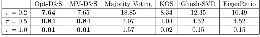
Opt-D&S MV-D&S Majority Voting KOS Ghosh-SVD EigenRatio

π = 0.2 7.64 7.65 18.85 8.34 12.35 10.49

π = 0.5 0.84 0.84 7.97 1.04 4.52 4.52 π = 1.0 0.01 0.01 1.57 0.02 0.15 0.15

Table 1: Prediction error (%) on the synthetic dataset. The parameter π indicates the sparsity of data—it is the probability that the worker labels each task.

It is worth contrasting condition (11) with condition (16), namely the sufficient con-ditions for the general model and for the one-coin model. It turns out that the one-coin model requires much milder conditions on the number of items. In particular, κ3 will be close to 1 if among all the workers there are three experts giving high-quality answers. As a consequence, the one-coin model is more robust than the general model. By contrasting the convergence rate ofµ_bil (by Theorem 4) andpbi (by Theorem 6), the convergence rate of

b

pi does not depend on{wl}k_l=1. This is additional evidence that the one-coin model enjoys a better convergence rate because of its simplicity.

7. Experiments

In this section, we report the results of empirical studies comparing the algorithm we propose in Section4(referred to as Opt-D&S) with a variety of other methods. We compare to the Dawid & Skene estimator initialized by majority voting (refereed to as MV-D&S), the pure majority voting estimator, the multi-class labeling algorithm proposed by Karger et al. (2013) (referred to as KOS), the SVD-based algorithm proposed by Ghosh et al. (2011) (referred to as Ghost-SVD) and the “Eigenvalues of Ratio” algorithm proposed by Dalvi et al.(2013) (referred to as EigenRatio). The evaluation is made on three synthetic datasets and five real datasets.

7.1 Synthetic data

For synthetic data, we generate m = 100 workers and n = 1000 binary tasks. The true label of each task is uniformly sampled from{1,2}. For each worker, the 2-by-2 confusion matrix is generated as follow: the two diagonal entries are independently and uniformly sampled from the interval [0.3,0.9], then the non-diagonal entries are determined to make the confusion matrix columns sum to 1. To simulate a sparse dataset, we make each worker label a task with probabilityπ. With the choiceπ ∈ {0.2,0.5,1.0}, we obtain three different datasets.

We execute every algorithm independently ten times and average the outcomes. For the Opt-D&S algorithm and the MV-D&S estimator, the estimation is outputted after ten EM iterates. For the group partitioning step involved in the Opt-D&S algorithm, the workers are randomly and evenly partitioned into three groups.

1 4 7 10 0.08

0.1 0.12 0.14 0.16 0.18

Number of iterations

Label prediction error

Opt−D&S MV−D&S

1 4 7 10

1 2 3 4 5 6

Number of iterations

Confusion matrix error

Opt−D&S MV−D&S

(a) (b)

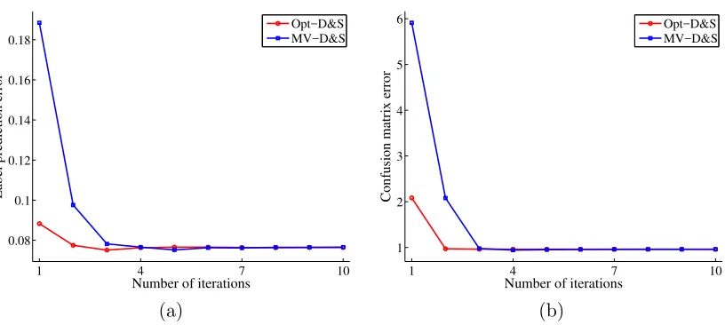
Figure 1: Comparing the convergence rate of the Opt-D&S algorithm and the MV-D&S es-timator on synthetic dataset withπ= 0.2: (a) convergence of the prediction error. (b) convergence of the squared error Pm

i=1kCb_i−C_ik2_F for estimating confusion matrices.

methods are consistently worse. It is not surprising that the Opt-D&S algorithm and the MV-D&S estimator yield similar accuracies, since they optimize the same log-likelihood objective. It is also meaningful to look at the convergence speed of both methods, as they employ distinct initialization strategies. Figure1 shows that the Opt-D&S algorithm converges faster than the MV-D&S estimator, both in estimating the true labels and in estimating confusion matrices. This can be explained by the general theoretical guarantee associated with Opt-D&S (recall Theorem 3).

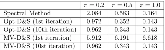
π = 0.2 π= 0.5 π = 1.0

Spectral Method 2.084 0.583 0.164

Opt-D&S (1st iteration) 0.972 0.352 0.143 Opt-D&S (10th iteration) 0.962 0.343 0.143 MV-D&S (1st iteration) 5.912 6.191 6.618 MV-D&S (10st iteration) 0.962 0.343 0.143

Table 2: Squared error for estimating the confusion matrix. The table compares (1) spectral method; (2) spectral initialization + one iteration of EM; (3) spectral initialization + 10 iterations of EM; (4) majority voting initialization + one iteration of EM; and (5) majority voting initialization + 10 iterations of EM.

Dataset name # classes # items # workers # worker labels

Bird 2 108 39 4,212

RTE 2 800 164 8,000

TREC 2 19,033 762 88,385

Dog 4 807 52 7,354

Web 5 2,665 177 15,567

Table 3: The summary of datasets used in the real data experiment.

7.2 Real data

For real data experiments, we compare crowdsourcing algorithms on five datasets: three binary tasks and two multi-class tasks. Binary tasks include labeling bird species ( Welin-der et al., 2010) (Bird dataset), recognizing textual entailment (Snow et al., 2008) (RTE dataset) and assessing the quality of documents in TREC 2011 crowdsourcing track (Lease and Kazai, 2011) (TREC dataset). Multi-class tasks include labeling the bread of dogs from ImageNet (Deng et al.,2009) (Dog dataset) and judging the relevance of web search results (Zhou et al.,2012) (Web dataset). The statistics for the five datasets are summa-rized in Table 3. Since the Ghost-SVD algorithm and the EigenRatio algorithm work on binary tasks, they are evaluated on the Bird, RTE and TREC dataset. For the MV-D&S estimator and the Opt-D&S algorithm, we iterate their EM steps until convergence.

Since entries of the confusion matrix are positive, we find it helpful to incorporate this prior knowledge into the initialization stage of the Opt-D&S algorithm. In particular, when estimating the confusion matrix entries by equation (5), we add an extra checking step before the normalization, examining if the matrix components are greater than or equal to a small threshold ∆. For components that are smaller than ∆, they are reset to ∆. The default choice of the thresholding parameter is ∆ = 10−6. Later, we will compare the Opt-D&S algorithm with respect to different choices of ∆. It is important to note that this modification doesn’t change our theoretical result, since the thresholding step doesn’t take effect if the initialization error is bounded by Theorem3.

Opt-D&S MV-D&S Majority Voting KOS Ghosh-SVD EigenRatio

Bird 10.09 11.11 24.07 11.11 27.78 27.78

RTE 7.12 7.12 10.31 39.75 49.13 9.00

TREC 29.80 30.02 34.86 51.96 42.99 43.96

Dog 16.89 16.66 19.58 31.72 – –

Web 15.86 15.74 26.93 42.93 – –

Table 4: Error rate (%) in predicting the true labels on real data.

10−6

10−5

10−4

10−3

10−2

10−1

0.08 0.1 0.12 0.14 0.16 0.18 0.2 0.22

Threshold

Label prediction error

Opt−D&S: 1st iteration Opt−D&S: 50th iteration MV−D&S: 1st iteration MV−D&S: 50th iteration

10−6 10−5

10−4 10−3

10−2 10−1 0.15

0.16 0.17 0.18 0.19 0.2 0.21

Threshold

Label prediction error

Opt−D&S: 1st iteration Opt−D&S: 50th iteration MV−D&S: 1st iteration MV−D&S: 50th iteration

10−6 10−5

10−4 10−3

10−2 10−1 0.15

0.2 0.25 0.3 0.35

Threshold

Label prediction error

Opt−D&S: 1st iteration Opt−D&S: 50th iteration MV−D&S: 1st iteration MV−D&S: 50th iteration

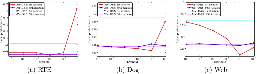
(a) RTE (b) Dog (c) Web

Figure 2: Comparing the MV-D&S estimator the Opt-D&S algorithm with different thresh-olding parameter ∆. The predict error is plotted after the 1st EM update and after convergence.

poorer performance, presumably due to the fact that they rely on idealized assumptions that are not met by the real data. In Figure 2, we compare the Opt-D&S algorithm with respect to different thresholding parameters ∆ ∈ {10−i}6

i=1. We plot results for three datasets (RET, Dog, Web), where the performance of the MV-D&S estimator is equal to or slightly better than that of Opt-D&S. The plot shows that the performance of the Opt-D&S algorithm is stable after convergence. But when only using the spectral method with just one E-step for the label prediction (i.e., the red curve Opt-D&S: 1st iterationin Figure 2), the error rates are more sensitive to the choice of ∆. A proper choice of ∆ makes the Opt-D&S algorithm perform better than MV-Opt-D&S. The result suggests that a proper spectral initialization with just an E-step is good enough for the purposes of prediction. In practice, the best choice of ∆ can be obtained by cross validation.

8. Conclusions

Under the generative model proposed by Dawid and Skene(1979), we propose an optimal algorithm for inferring true labels in the multi-class crowd labeling setting. Our approach utilizes the method of moments to construct an initial estimator for the EM algorithm. We proved that our method achieves the optimal rate with only one iteration of the EM algorithm.

One-step EM initialized by the method of moments not only leads to better estimation error in terms of the dependence on the condition number of the second-order moment matrix but it also computationally more attractive than the standard one-step estimator obtained via a Newton-Raphson step. It is interesting to explore whether a properly initialized one-step EM algorithm can achieve the optimal rate for other latent variable models such as latent Dirichlet allocation or other mixed membership models.

Acknowledgments

Appendix A. Proof of Theorem 3

If a 6=b, it is easy to verify that Sab =CaW(Cb)T =E[Zaj⊗Zbj]. Furthermore, we can upper bound the spectral norm ofSab, namely

kSabkop≤

k X

l=1

wlkµalk2kµ blk2 ≤

k X

l=1

wlkµalk1kµ

blk1≤1. For the same reason, it can be shown that kTabckop≤1.

Our proof strategy is briefly described as follows: we upper bound the estimation error for computing empirical moments (2a)-(2d) in Lemma 7, and upper bound the estimation error for tensor decomposition in Lemma8. Then, we combine both lemmas to upper bound the error of formula (5).

Lemma 7 Given a permutation (a, b, c) of (1,2,3), for any scalar ≤ σL/2, the second

and the third moments M2c and M3c computed by equation (2c) and (2d) are bounded as

max{kMc₂−M₂kop,kMc₃−M₃kop} ≤31/σ

3

L (17)

with probability at least 1−δ, where δ = 6 exp(−(√n−1)2) +kexp(−(pn/k−1)2).

Lemma 8 Suppose that (a, b, c) is permutation of (1,2,3). For any scalar ≤κ/2, if the empirical moments M2c and M3c satisfy

max{kM2c −M2kop,kM3c −M3kop} ≤H (18)

for H := min (

1 2,

2σ3_L/2

15k(24σ_L−1+ 2√2),

σ_L3/2

4p3/2σ_L1/2+ 8k(24/σL+ 2

√

2) )

then the estimatesCb_c and Wc are bounded as

kCb_c−C_ckop≤

√

k and kWc−Wkop≤.

with probability at least 1−δ, where δ is defined in Lemma 7.

Combining Lemma 7, Lemma 8, if we choose a scalar1 satisfying

1 ≤min{κ/2, πminwminσL/(36k)}, (19) then the estimatesCb_g (forg= 1,2,3) and Wc satisfy

kCb_g−C_gkop≤

√

k1 and kWc−Wkop≤1. (20) with probability at least 1−6δ, where

δ = (6 +k) exp−(pn/k1Hσ3L/31−1)2

To be more precise, we obtain the bound (20) by plugging := 1Hσ3L/31 into Lemma 7, then plugging :=1 into Lemma8. The high probability statement is obtained by apply-ing a union bound.

Assuming inequality (20), for any a ∈ {1,2,3}, since kC_akop ≤

√

k,kCb_a−C_akop ≤

√

k1 and kWkop ≤ 1,

Wc−W

op

≤ 1, Lemma 18 (the preconditions are satisfied by inequality (19)) implies that

cWCb

a−W Ca op ≤4 √ k1,

Since condition (19) implies

kcWCb_a−W C_akop≤4

√

k1≤√wminσL/2≤σk(W Ca)/2

Lemma17 yields that

c WCb_a

−1

−(W C_a)−1 op ≤ 8 √ k1 wminσL

.

By Lemma19, for anyi∈[m], the concentration bound

1 n n X j=1

zijZajT −E[zijZajT] op ≤1

holds with probability at least 1−mexp(−(√n1−1)2). Combining the above two inequal-ities with Proposition2, then applying Lemma 18with preconditions

(W C_a)−1

op≤

1 wminσL

and E

zijZajT

op≤1,

we have 1 n n X j=1 zijZajT

c WCb_a

−1

| {z }

b

G

−πiCi op ≤ 18 √ k1 wminσL

. (21)

LetGb ∈_Rk×k be the first term on the left hand side of inequality (21). Each column of Gb, denoted byGb_l, is an estimate ofπ_iµ_il. The`₂-norm estimation error is bounded by 18

√ k1

wminσL.

Hence, we have

kGb_l−π_iµ_ilk₁ ≤

√

kkGb_l−π_iµ_ilk₂ ≤

√

kkGb−π_iC_ikop≤

18k1 wminσL

and consequently, using the fact that Pk

c=1µilc= 1, we have

normalize(Gbl)−µil

2=

b Gl πi+Pk_c=1

b

Glc−πiµilc −µil

2

≤ kGbl−πiµilk2+kGbl−πiµilk1kµilk2

πi− kGb_l−π_iµ_ilk₁

≤ 72k1

πminwminσL

(23)

where the last step combines inequalities (21), (22) with the bound 18k1

wminσL ≤ πi/2 from

condition (19), and uses the fact thatkµilk2≤1.

Note that inequality (23) holds with probability at least

1−(36 + 6k) exp−(pn/k1HσL3/31−1)2

−mexp(−(√n1−1)2).

It can be verified that H≥ σ

5/2

L

230k. Thus, the above expression is lower bounded by 1−(36 + 6k+m) exp

−

√

n1σ11_L/2 31×230·k3/2 −1

2 ,

If we represent this probability in the form of 1−δ, then

1 = 31×230·k 3/2

√

nσ_L11/2

1 +plog((36 + 6k+m)/δ)

. (24)

Combining condition (19) and inequality (23), we find that to makekCb−Ck∞ bounded by , it is sufficient to choose1 such that

1≤min nπ

minwminσL 72k ,

κ 2,

πminwminσL 36k

o

This condition can be further simplified to

1 ≤

πminwminσL

72k (25)

for small, that is≤minn_π 36κk

minwminσL,2

o

. According to equation (24), the condition (25) will be satisfied if

√

n≥ 72×31×230·k

5/2 πminwminσ

13/2 L

1 +plog((36 + 6k+m)/δ)

.

A.1 Proof of Lemma 7

Throughout the proof, we assume that the following concentration bound holds: for any distinct indices (a0, b0)∈ {1,2,3}, we have

1 n n X j=1

Za0_j⊗Z_b0_j−_E[Z_a0_j⊗Z_b0_j]

op

≤. (26)

By Lemma 19 and the union bound, this event happens with probability at least 1−

6 exp(−(√n−1)2). By the assumption that ≤ σL/2 ≤ σk(Sab)/2 and Lemma 17, we have 1 n n X j=1

Zcj⊗Zbj−E[Zcj⊗Zbj] op

≤ and

  1 n n X j=1

Zaj⊗Zbj 

 −1

−(E[Zaj⊗Zbj])−1 op ≤ 2 σ2 k(Sab)

Under the preconditions

kE[Zcj⊗Zbj]k_op≤1 and

(E[Z_aj⊗Zbj])−1

op≤

1 σk(Sab)

,

Lemma18 implies that

  1 n n X j=1

Zcj⊗Zbj     1 n n X j=1

Zaj⊗Zbj 

 −1

−_E[Zcj⊗Zbj](E[Zaj⊗Zbj])−1 op ≤2 σk(Sab)

+ 2

σ2 k(Sab)

≤6/σ2_L (27)

and for the same reason, we have

  1 n n X j=1

Zcj⊗Zaj     1 n n X j=1

Zbj⊗Zaj 

 −1

−E[Zcj⊗Zaj](E[Zbj⊗Zaj])−1 op

≤6/σ_L2 (28)

Now, let matricesF2 and F3 be defined as

F2:=E[Zcj⊗Zbj](E[Zaj⊗Zbj])−1, F3:=E[Zcj⊗Zaj](E[Zbj⊗Zaj])−1,

and let the matrix on the left hand side of inequalities (27) and (28) be denoted by ∆2 and ∆3, we have

Zb

0

aj⊗Zb_bj0 −F₂(Z_aj⊗Z_bj)F₃T op =

F2+ ∆2

(Zaj⊗Zbj)

F3+ ∆3 T

−F2(Zaj⊗Zbj)F3T

op

≤ kZaj⊗Zbjkop k∆2kopkF3+ ∆2kop+kF2kopk∆3kop

≤30kZaj⊗Zbjkop/σ

where the last steps uses inequality (27), (28) and the fact that max{kF2kop,kF3kop} ≤1/σL

and

kF3+ ∆2kop≤ kF3kop+k∆2kop≤1/σL+ 6/σL2 ≤4/σL. To upper bound the normkZaj⊗Zbjkop, notice that

kZaj⊗Zbjkop≤ kZajk2kZbjk2≤ kZajk1kZbjk1 ≤1. Consequently, we have

Zb

0

aj⊗Zb_bj0 −F₂(Z_aj⊗Z_bj)F₃T

op

≤30/σ_L3. (29)

For the rest of the proof, we use inequality (29) to bound M2c and M3c. For the second moment, we have

Mc2−M2 op ≤ 1 n n X j=1 Zb 0

aj⊗Zb_bj0 −F₂(Z_aj⊗Z_bj)F₃T op + F2   1 n n X j=1

Zaj⊗Zbj 

F₃T −M2 op

≤30/σ3_L+ F2   1 n n X j=1

Zaj⊗Zbj−E[Zaj⊗Zbj] 

F₃T op

≤30/σ3_L+/σ_L2 ≤31/σ_L3. For the third moment, we have

c

M3−M3= 1 n n X j=1 b

Z_aj0 ⊗Zb_bj0 −F₂(Z_aj⊗Z_bj)F₃T

⊗Zcj

+   1 n n X j=1

F2(Zaj⊗Zbj)F3T ⊗Zcj−EF2(Zaj⊗Zbj)F3T ⊗Zcj



. (30)

We examine the right hand side of equation (30). The first term is bounded as

b

Z_aj0 ⊗Zb_bj0 −F₂(Z_aj⊗Z_bj)F₃T

⊗Zcj op ≤ Zb 0

aj⊗Zb_bj0 −F₂(Z_aj⊗Z_bj)F₃T

op

kZcjk₂

≤30/σ_L3. (31)

For the second term, since kF2Zajk2 ≤1/σL,kF3Zbjk2 ≤1/σL and kZcjk2 ≤1, Lemma 19 implies that 1 n n X j=1

F2(Zaj⊗Zbj)F3T ⊗Zcj−EF2(Zaj⊗Zbj)F3T ⊗Zcj op

≤/σ2_L (32)

with probability at least 1−kexp(−(pn/k−1)2). Combining inequalities (31) and (32), we have

M3c −M3

op

≤30/σ3_L+/σ_L2 ≤31/σ_L3.

A.2 Proof of Lemma 8

Chaganty and Liang (2013) (Lemma 4) prove that when condition (18) holds, the tensor decomposition method of Algorithm 1 outputs {µ_bh,wbh}

k

h=1, such that with probability at least 1−δ, a permutation π satisfies

k_bµ_h−µ_{cπ (h)}k2≤ and

w_bh−w_π(h)

∞≤.

Note that the constant H in Lemma 8 is obtained by plugging upper bounds kM2kop ≤1

and kM3kop≤1 into Lemma 4 of Chaganty and Liang(2013).

Theπ(h)-th component ofµ_cπ(h)is greater than other components ofµ_cπ(h), by a margin of κ. Assuming ≤ κ/2, the greatest component of µb

h is its π(h)-th component. Thus, Algorithm 1 is able to correctly estimate the π(h)-th column of Cb_c by the vector _bµ_h. Consequently, for every column ofCb_c, the`₂-norm error is bounded by. Thus, the spectral-norm error ofCb_c is bounded by

√

k. SinceW is a diagonal matrix andw_bh−w_π(h)

∞≤, we have kWc−Wkop≤.

Appendix B. Proof of Theorem 4

We define three random events that will be shown holding with high probability:

E₁ : m X

i=1 k X

c=1

I(zij =ec) log(µiyjc/µilc)≥mD/2 for all j∈[n] and l∈[k]\{yj}.

E2 :

n X

j=1

I(yj =l)I(zij =ec)−nwlπiµilc

≤ntilc for all (i, l, c)∈[m]×[k] 2_.

E3 :

n X

j=1

I(yj =l)I(zij 6= 0)−nwlπi ≤

ntilc µilc

for all (i, l, c)∈[m]×[k]2_{. (33)}

where tilc >0 are scalars to be specified later. We define tmin to be the smallest element

among {tilc}. Assuming that E1 ∩ E2 holds, the following lemma shows that performing updates (7) and (8) attains the desired level of accuracy. See SectionB.1 for the proof.

Lemma 9 Assume that E₁∩ E₂ holds. Also assume thatµilc≥ρ for all(i, l, c)∈[m]×[k]2.

If Cb is initialized such that inequality (10) holds, and scalars t_ilc satisfy

2 exp−mD/4 + log(k)≤tilc≤πminwminmin

ρ 8,

ρD 64

. (34)

Then by alternating updates (7) and (8) for at least one round, the estimates Cb and q_bare

bounded as

|µ_bilc−µilc| ≤4tilc/(πiwl). for all i∈[m],l∈[k], c∈[k]. max

l∈[k]

{|q_bjl−I(yj =l)|} ≤exp −mD/4 + log(k)

Next, we characterize the probability that eventsE₁,E₂andE₃hold. For measuringP[E1], we define auxiliary variable si := Pk_c=1I(zij = ec) log(µiyjc/µilc). It is straightforward to

see that s1, s2, . . . , sm are mutually independent on any value ofyj, and each si belongs to the interval [0,log(1/ρ)]. it is easy to verify that

E " _m X i=1 si yi # = m X i=1

πiDKL µiyj, µil

.

We denote the right hand side of the above equation by D. The following lemma shows that the second moment ofsi is bounded by the KL-divergence between labels.

Lemma 10 Conditioning on any value ofyj, we have

E[s2i|yi]≤

2 log(1/ρ)

1−ρ πiDKL µiyj, µil

.

According to Lemma 10, the aggregated second moment of si is bounded by

E "_m

X

i=1 s2_i

yi

#

≤ 2 log(1/ρ)

1−ρ m X

i=1

πiDKL µiyjc, µilc

= 2 log(1/ρ) 1−ρ D

Thus, applying the Bernstein inequality, we have

P h X

i=1

si≥D/2|yi i

≥1−exp 

−

1 2(D/2)

2 2 log(1/ρ)

1−ρ D+ 1

3(2 log(1/ρ))(D/2) 

,

Since ρ ≤ 1/2 and D ≥ mD, combining the above inequality with the union bound, we have

P[E1]≥1−knexp

− mD

33 log(1/ρ)

. (35)

For measuringP[E2], we observe thatPnj=1I(yj =l)I(zij =ec) is the sum ofni.i.d. Bernoulli random variables with meanp:=πiwlµilc. Sincetilc≤πminwminρ/8≤p, applying the

Cher-noff bound implies

P   n X j=1

I(yj =l)I(zij =ec)−np

≥ntilc 

≤2 exp(−nt2_ilc/(3p)) = 2 exp

− nt

2 ilc 3πiwlµilc

,

For measuring P[E3], note that Pn_j=1I(yj =l)I(zij 6=ec) is the sum of ni.i.d. Bernoulli random variables with mean q := πiwl. Since _µtilc_ilc ≤ πminw_ρminρ/8 ≤ q, using a Chernoff bound yields P   n X j=1

I(yj =l)I(zij 6= 0)−nq ≥n tilc µilc 

≤2 exp(− nt2_ilc 3qµ2

ilc

)≤2 exp

− nt

2 ilc 3πiwlµilc

,

Summarizing the probability bounds on E1, E2 and E3, we conclude that E1 ∩ E2 ∩ E3 holds with probability at least

1−knexp

− mD

33 log(1/ρ) − m X i=1 k X l=1 4 exp − nt 2 ilc 3πiwlµilc

Proof of Part (a) According to Lemma 9, for y_bj =yj being true, it sufficient to have exp(−mD/4 + log(k))<1/2, or equivalently

m >4 log(2k)/D. (37)

To ensure that this bound holds with probability at least 1−δ, expression (36) needs to be lower bounded byδ. It is achieved if we have

m≥ 33 log(1/ρ) log(2kn/δ)

D and n≥

3πiwlµilclog(8mk/δ)

t2_ilc (38) If we choose

tilc := r

3πiwlµilclog(8mk/δ)

n . (39)

then the second part of condition (38) is guaranteed. To ensure that tilc satisfies condi-tion (34). We need to have

r

3πiwlµilclog(8mk/δ)

n ≥2 exp

−mD/4 + log(k) and r

3πiwlµilclog(8mk/δ)

n ≤πminwminα/4. The above two conditions require that m andn satisfy

m≥ 4 log(2k

p

n/(3πminwminρlog(8mk/δ)))

D (40)

n≥ 48 log(8mk/δ)

πminwminα2

(41)

The four conditions (37), (38), (40) and (41) are simultaneously satisfied if we have

m≥ 33 log(1/ρ) log(2kn/δ)

D and n≥ 48 log(8mk/δ)

πminwminα2

.

Under this setup, byj =yj holds for all j∈[n] with probability at least 1−δ.

Proof of Part (b) Iftilcis set by equation (39), combining Lemma9with this assignment, we have

(µ_bilc−µilc)2 ≤

48µilclog(8mk/δ) πiwln

B.1 Proof of Lemma 9

To prove Lemma 9, we study the consequences of update (7) and update (8). We prove two important lemmas, which show that both updates provide good estimates if they are properly initialized.

Lemma 11 Assume that eventE₁ holds. If µand its estimate µ_b satisfy

µilc≥ρ and |µbilc−µilc| ≤δ1 for all i∈[m], l∈[k], c∈[k], (42)

and q_bis updated by formula (7), then q_bis bounded as:

max l∈[k]

{|q_bjl−I(yj =l)|} ≤exp

−m

D 2 −

2δ1 ρ−δ1

+ log(k)

for allj∈[n]. (43)

Proof

For an arbitrary index l6=yj, we consider the quantity

Al:= m X i=1 k X c=1

I(zij =ec) log(µbiyjc/µbilc)

By the assumption that E1 and inequality (42) holds, we obtain that

Al= m X i=1 k X c=1

I(zij =ec) log(µiyjc/µilc) +

m X i=1 k X c=1

I(zij =ec)

log

b µiyjc

µiyjc

−log b µilc µilc ≥ m X i=1

πiDKL µiyj, µil

2

!

−2mlog ρ

ρ−δ1 ≥m D 2 − 2δ1 ρ−δ1

. (44)

Thus, for every indexl6=yj, combining formula (7) and inequality (44) implies that

b qjl≤

1 exp(Al)

≤exp −m D 2 − 2δ1 ρ−δ1

.

Consequently, we have

b

qjyj ≥1−

X

l6=yj

b

qjl≥1−kexp −m D 2 − 2δ1 ρ−δ1

.

Combining the above two inequalities completes the proof.

Lemma 12 Assume that eventE2 holds. If bq satisfies max

l∈[k]

{|q_bjl−I(yj =l)|} ≤δ2 for allj∈[n], (45)

and µbis updated by formula (8), then µb is bounded as:

|µ_bilc−µilc| ≤

2ntilc+ 2nδ2 (7/8)nπiwl−nδ2

Proof By formula (8), we can writeµ_bilc=A/B, where A:= n X j=1 b

qjlI(zij =ec) and B := k X

c0₌₁

n X

j=1 b

qjlI(zij =ec0) =

n X

j=1 b

qjlI(zij 6= 0).

Combining this definition with the assumption that event E2 and inequality (45) hold, we find that

|A−nπiwlµilc| ≤

n X j=1

I(qjl =yj)I(zij=ec)−nπiwlµilc

+ n X j=1 b

qjlI(zij =ec)−

n

X

j=1

I(qjl=yj)I(zij =ec)

≤ntilc+nδ2.

Similarly, using the assumption that event E3 and inequality (45) hold, we have

|B−nπiwl| ≤ n X j=1

I(qjl=yj)I(zij 6= 0)−nπiwl + n X j=1 b

qjlI(zij 6= 0)− n X

j=1

I(qjl=yj)I(zij 6= 0)

≤ ntilc

µilc

+nδ2.

Combining the bound for A andB, we obtain that

|µ_bilc−µilc|=

nπiwlµilc+ (A−nπiwlµilc) nπiwl+ (B−nπiwl)

−µilc =

(A−nπiwlµilc)−µilc(B−nπiwl) nπiwl+ (B−nπiwl)

≤ 2ntilc+ 2nδ2

nπiwl−n(tilc/µilc)−nδ2 .

Condition (34) implies

tilc µilc

≤ tilc

ρ ≤

πminwminρ

8ρ =

πminwmin

8 ,

lower bounding the denominator. Plugging in this bound completes the proof.

To proceed with the proof, we assign specific values to δ1 and δ2. Let

δ1:= min ρ 2, ρD 16

and δ2 :=tmin/2. (47)

We claim that at any step in the update, the preconditions (42) and (45) always hold. We prove the claim by induction. Before the iteration begins, µb is initialized such that the accuracy bound (10) holds. Thus, condition (42) is satisfied at the beginning. We assume by induction that condition (42) is satisfied at time 1,2, . . . , τ−1 and condition (45) is satisfied at time 2,3, . . . , τ−1. At time τ, either update (7) or update (8) is performed. If update (7) is performed, then by the inductive hypothesis, condition (42) holds before the update. Thus, Lemma 11 implies that

max

l∈[k]{|qbjl−I(yj =l)|} ≤exp −m D 2 − 2δ1 ρ−δ1

+ log(k)

The assignment (47) implies D₂ − 2δ1

ρ−δ1 ≥

D

4, which yields that max

l∈[k]

{|q_bjl−I(yj =l)|} ≤exp(−mD/4 + log(k))≤tmin/2 =δ2,

where the last inequality follows from condition (34). It suggests that condition (45) holds after the update.

On the other hand, we assume that update (8) is performed at timeτ. Since update (8) follows update (7), we haveτ ≥2. By the inductive hypothesis, condition (45) holds before the update, so Lemma12 implies

|µ_bilc−µilc| ≤

2ntilc+ 2nδ2 (7/8)nπiwl−nδ2

= 2ntilc+ntmin (7/8)nπiwl−ntmin/2

≤ 3ntilc

(7/8)nπiwl−ntmin/2

,

where the last step follows sincetmin ≤tilc. Noticingρ≤1, condition (34) implies thattmin≤

πminwmin/8. Thus, the right hand side of the above inequality is bounded by 4tilc/(πiwl). Using condition (34) again, we find

4tilc πiwl

≤ 4tilc

πminwmin

≤min

ρ 2,

ρD 16

=δ1,

which verifies that condition (42) holds after the update. This completes the induction.

Since preconditions (42) and (45) hold for any time τ ≥2, Lemma 11 and Lemma 12 implies that the concentration bounds (43) and (46) always hold. These two concentration bounds establish the lemma’s conclusion.

B.2 Proof of Lemma 10

By the definition ofsi, we have

E[s2i] =πi k X

c=1

µiyjc(log(µiyjc/µilc))

2 _=π i

k X

c=1

µiyjc(log(µilc/µiyjc))

2

We claim that for anyx≥ρ and ρ <1, the following inequality holds:

log2(x)≤ 2 log(1/ρ)

1−ρ (x−1−log(x)). (48)

We defer the proof of inequality (48), focusing on its consequence. Let x:=µilc/µiyjc, then

inequality (48) yields that

E[s2i]≤

2 log(1/ρ) 1−ρ πi

k X

c=1

µilc−µiyjc−µiyjclog(µilc/µiyjc)

!

= 2 log(1/ρ)

1−ρ πiDKL µiyj, µil

.

It remains to prove the claim (48). Let f(x) := log2(x)− 2 log(1_1−ρ/ρ)(x−1−log(x)). It suffices to show that f(x)≤0 for x≥ρ. First, we havef(1) = 0 and

f0(x) = 2(log(x)

For anyx >1, we have

log(x)< x−1≤ log(1/ρ)

1−ρ (x−1)

where the last inequality holds since log(1/ρ) ≥ 1−ρ. Hence, we have f0(x) < 0 and consequently f(x)<0 forx >1.

For any ρ ≤x <1, notice that log(x)−log(1_1−ρ/ρ)(x−1) is a concave function of x, and equals zero at two points x= 1 and x=ρ. Thus, f0(x) ≥0 at any pointx∈[ρ,1), which implies f(x)≤0.

Appendix C. Proof of Theorem 5

In this section we prove Theorem5. The proof separates into two parts.

C.1 Proof of Part (a)

Throughout the proof, probabilities are implicitly conditioning on {πi} and {µilc}. We assume that (l, l0) are the pair of labels such that

D= 1 m

m X

i=1

πiDKL(µil, µil0).

LetQ be a uniform distribution over the set{l, l0}n. For any predictorby, we have

max v∈[k]nE

h_Xn

j=1

I(ybj 6=yj) y=v

i

≥ X

v∈{l,l0_}n

Q(v)E h_Xn

j=1

I(ybj 6=yj) y=v

i

= n X

j=1 X

v∈{l,l0_}n

Q(v)E h

I(byj 6=yj) y=v

i

. (49)

Thus, it is sufficient to lower bound the right hand side of inequality (49). For the rest of the proof, we lower bound the quantityP

y∈{l,l0_}n_Q(v)_E[_I(_byj 6=yj)|y] for every itemj. LetZ :={zij :i∈[m], j ∈[n]}be the set of all observations. We define two probability measures P0 and P1, such that P0 is the measure of Z conditioning on yj =l, while P1 is the measure of Z conditioning on yj =l0. By applying Le Cam’s method (Yu, 1997) and Pinsker’s inequality, we have

X

v∈{l,l0_}n

Q(v)E h

I(ybj 6=yj) y=v

i

=Q(yj =l)P0(ybj 6=l) +Q(yj =l 0₎

P1(ybj 6=l 0₎

≥ 1

2 − 1

2kP0−P1kTV

≥ 1

2 − 1 4

p

P0 and P1. Letting the distribution ofX with respect to probability measureP be denoted

by P(X), we have

DKL(P0,P1) =DKL(P0(Zj),P1(Zj)) +DKL(P0(Z\Zj),P1(Z\Zj)) =DKL(P0(Zj),P1(Zj)), (51)

where the last step follows sinceP0(Z\Zj) =P1(Z\Zj). Next, we observe thatz1j, z2j, . . . , zmj are mutually independent given yj, which implies

DKL(P0(Zj),P1(Zj)) = m X

i=1

DKL(P0(zij),P1(zij))

= m X

i=1 "

(1−πi) log

1−πi 1−πi

+

k X

c=1

πiµilclog

πiµilc πiµil0_c

#

= m X

i=1 k X

c=1

πiDKL(µilc, µil0_c) =mD. (52)

Combining inequality (50) with equations (51) and (52), we have

X

v∈{l,l0_}n

Q(v)E h

I(byj 6=yj) y =v

i

≥ 1

2− 1 4

p mD.

Thus, if m ≤ 1/(4D), then the above inequality is lower bounded by 3/8. Plugging this lower bound into inequality (49) completes the proof.

C.2 Proof of Part (b)

Throughout the proof, probabilities are implicitly conditioning on{πi}and{wl}. We define two vectors

u0 :=

1 2,

1

2,0, . . . ,0 T

∈_Rk and u1 :=

1 2 +δ,

1

2 −δ,0, . . . ,0 T

∈_Rk,

whereδ ≤1/4 is a scalar to be specified. Consider am-by-krandom matrixV whose entries are uniformly sampled from {0,1}. We define a random tensor uV ∈ Rm×k×k, such that

(uV)il :=uVil for all (i, l)∈[m]×[k]. Givan an estimator µband a pair of indices (¯i,¯l), we have

sup µ∈Rm×k×k

E h

kµ¯_bi¯_l−µ¯_i¯_lk2₂ i

≥ X

v∈[k]n

P(y=v) X

V

P(V)E h

kµ¯_bi¯_l−µ¯_i¯_lk2₂

µ=uV, y=v i

! .

(53)

For the rest of the proof, we lower bound the termP

V P(V)E[kµ¯bi¯l−µ¯i¯lk 2

2|µ=uV, y= v] for everyv∈[k]n_{. Let}

b

V be an estimator defined as

b V =