FORECASTING TECHNIQUES, OPERATING ENVIRONMENT AND ACCURACY OF PERFORMANCE FORECASTING FOR LARGE MANUFACTURING FIRMS IN KENYA

(1)

http: // www.gjesrm.com (C) Global Journal of Engineering Science and Research Management

FORECASTING

TECHNIQUES,

OPERATING

ENVIRONMENT

AND

ACCURACY

OF

PERFORMANCE FORECASTING FOR LARGE MANUFACTURING FIRMS IN KENYA

E. W. Chindia*1_{F. N. Kibera}2

*1_{PhD, Investment Consultant, Graduate, School of Business, University of Nairobi, P.O. Box 4577 - 00506, Nairobi. Kenya.} 2_{PhD, Prof., School of Business, University of Nairobi, P.O. Box 30197 - 00100, Nairobi. Kenya.}

*Correspondence Author: [email protected]

Keywords:

Forecasting techniques, operating environment, accuracy of performance forecasting, large manufacturing firms.

Abstract

This article explores the interaction between forecasting techniques (FT), operating environment (OE) and accuracy of performance forecasting (APF). Objectives were to compare FT in the APF, identify performance measures influenced by OE, assess moderating effects of the OE on the relationship between a FT and APF and examine relationships among FT, OE and APF. A model and framework are formed on the basis of previous research. Empirical testing of the model was done after collecting data using a structured questionnaire administered among randomly selected large manufacturing firms (LMF) in Kenya. Measures of APF included expected value (EV), return on sales (ROS), return on assets (ROA) and growth in market share (GMS). Objective, judgmental and combined FTs were used. Internal operating environment (IOE) comprised leadership, strategy, structure and culture; while customers, competitors, suppliers, substitute products and demographic characteristics constituted external operating environment (EOE). Empirical results indicate that the effect of objective and combined FT and EOE on APF was strong. Conversely, the effect of the IOE on APF was not strong. Further, the effect of the EOE accounted for more variation in APF compared to the IOE. Statistically significant were competitors and external customers on the influence of APF. The three FT yielded APF against EV and ROS. There was statistically significant evidence that (except for EV and ROS) EOE had an influence on APF. Regression analysis indicated that EOE had a partial moderating effect on the relationship between each of the FT and APF with respect to ROS and ROA for objective FT and ROA for both combined and judgmental FT. Alternatively, the IOE had a moderating effect on the relationship between objective FT and APF with respect to ROS; and the joint effect of the OE had a partial moderating effect on the relationship between objective and combined FT and APF with respect to EV and ROS. Results show that objective and combined FT yielded APF in a competitive environment. Hence, to achieve APF a FT should not ignore the effects of the OE. The study contributes by developing an exploratory model to link APF in LMF with variables of the OE.

Introduction

(2)

to efficient operations and high levels of customer service (Adam and Ebert, 2001). For new manufacturing facilities demand needs to be forecasted many years into the future since the facility will serve the firm for many years to come (Bails and Peppers, 1982).

Forecasting is therefore, a problem that arises in many economic and managerial contexts, but has become a challenging concept in the study of public and private enterprises. There is no agreement as to which method of forecasting to use and yet the selection and implementation of a proper forecasting technique has always been an important planning and control issue for firms. Often, the financial well-being of the entire operation relies on the APF since such information is used to make interrelated budgetary and operating decisions. In a dynamic and competitive environment businesses need to satisfy their customers and their shareholders by maintaining high levels of performance (Neely et al., 1995). The liberalization of the world economy has led to a reduction in trade barriers among countries leading to greater competition. Businesses have to collaborate with new global players (Stoner et al., 2001). Organizations which focused on local markets have extended their frontiers in terms of markets and production facilities. The context in which the management of forecasting is carried out has also changed rapidly. Globalization has led to significant emphasis on efficiency, productivity and competitiveness (Intriligator, 2001). However, all these firms need to operate in a more flexible and pro-reactive manner to market changes (Garengo, 2009; Hendry, 2001). Management thinkers have also talked about companies living in turbulence (Wadell and Shoal, 1994). For developing countries, the turbulence is severer due to unpredictable and inseparable political-economic environment, forced trade liberation, and implementation of structural adjustment programs. With rapid and often unpredictable changes in economic and market conditions, managers are making decisions without knowing what will exactly happen in future (Chan, 2000). Forecasting remains essential for decision making, unless insurance or hedging is selected to deal with the future (Armstrong, 1988). Good forecasts are a major input in all aspects of manufacturing operations decisions (Heizer and Render, 1991; Fildes and Hastings, 1994). Thomas and Dacosta (1979) and Carter (1987) assert that forecasting is the number one area of applications in corporations. Lambert and Stock (1993, p.559) positioned forecasting as the driving force behind all forward planning activities in firms. Accurate forecasts help companies prepare for short and long term changes in market conditions and improve operating performance (Fildes and Beard, 1992; Gardner, 1990; Wacker and Lummus, 2002). When the accuracy of forecasts declines, decisions based on the forecasts lead to operational miss-steps (Aviv, 2001, 2003; Gardner, 1990; Nachiappan et al., 2005; Ghodrati and Kumar, 2005).

The growing importance of the forecasting function within companies is reflected in the increased level of commitment in terms of money, hiring of operational researchers and statisticians, and purchasing computer software. In addition, the increasing complexity of organizations and their environments have made it more difficult for decision makers to take all factors regarding future development of organizations into account. Organizations have also moved towards more systematic decision making that involves explicit justifications for individual actions - formalized forecasting is one way in which actions can be supported (Wheelright and Clarke, 1976; Pan et al., 1977; Fildes and Hastings, 1994; Makridakis et al., 1983).

(3)

http: // www.gjesrm.com (C) Global Journal of Engineering Science and Research Management

Literature review

Competitive activity in LMFs has intensified requiring accuracy of forecasts in setting future goals. Market rivalry in this competitive environment can be high, moderate or low. The proposition in this study was that a selected forecasting method is dependent on the strength of the bargaining power in the competitive environment. While environmental factors are generally taken into account when a single FT is employed, it is proposed that when a FT changes the moderating effect of the operating environment behaves differently impacting APF. There are two main techniques to forecasting, qualitative, which is subjective and uses experience and judgment to establish future behaviors; and quantitative, which uses historical data to establish relationships and trends that can be projected into the future.

A third forecasting model can be crafted by combining subjective and objective techniques. The combination process is dependent on the accuracy of performance forecasting a firm aims to achieve by either minimizing the Mean Square Error (MSE) of the resulting FT or combining forecasts to attain a simple average of the different forecasts used in the combination. In each of these methods some amount of the effects of the operating environment is inherently factored in them, but the extent to which their impact is incorporated is not known and how the accuracy of these FTs is affected individually remains undetermined. The interaction effect of the operating environments on APF is not also quantified. In a judgmental forecasting, Smith and Mentzer (2010) observe that user perceptions and actions of forecasters have a significant influence on forecasts. This FT has been known to be helpful to the manufacturers of industrial products for preparing short-term forecasts. However, it is weak if there is trend or changes in the product or the market demand. It also suffers from lack of knowledge about the amount of environmental effects imported into the forecasts, particularly in turbulent markets. On the other hand, objective forecasting lends itself well to an abundance of data, although where consumer behavior and market patterns are erratic, the use of historical data alone becomes questionable.

Evidence exists that combining FTs can improve APF in various situations (Armstrong, 2001). There are also contrary views that combining forecasts on its own does not necessarily improve accuracy of forecasts (Larrick and Soll, 2003), but reliance on some input from practitioners in industry. Armstrong (2001) explains that combining forecasts refers to the averaging of independent forecasts and useful only when uncertain as to which method to apply or when current method alone is not providing an adequate measure of accuracy. He states that even if one method can be identified as best, combining still may be useful if the other methods contribute some meaningful information. The more that methods differ, the greater the expected improvement in accuracy over the average of the individual forecasts. Combining forecasts therefore, tends to even-out uncertainties within the different forecasts used, but erratic changes in market rivalry could render this method less accurate.

The effect of combining a more accurate forecast with a less accurate forecast may result in a lower than average forecast. However, many things affect forecasts and these might be captured by combining forecasts to reduce errors arising from faulty assumptions, bias, or mistakes in data. Research on time series forecasting argues that predictive performance increases through combined FTs (Armstrong, 1989, 2001; Clemen, 1989; Makridakis and Winkler, 1983; Makridakis et al., 1982; Terui and Van Dijk, 2002). In an experiment, Bunn and Taylor (2001) combined a judgmental method with a statistical model in which “improvements in accuracy were stated to have been considerable and difficult to benchmark”. In another time series experimental study, Hibon and Evgeniou (2005) conclude that selecting among combinations is less risky than selecting among individual forecasts. These studies did not consider conditions in high market rivalry and turbulent environment.

(4)

Performance. In a study of the improvement in the sales pipeline, Synader (2008) concluded that by incorporating the customer’s point of view into sales strategy accurate forecasts were a natural by-product of a good sales pipeline. In a survey of how user perceptions and actions influence forecasts, Smith and Mentzer (2010) conclude that combining FTs is still under-explored. According to Makridakis and Hibon (2000), New bold and Harvey (2002) and Hendry and Clements (2002), APF can be improved through a combination of forecasting methods. In the above studies, the impact of moderator effects on the relationship between a FT and APF was not explored. Smith and Mentzer (2010), Vieira and Favaretto (2006), Makridakis et al. (1983) and Schultz (1992) underscored the fact that forecasting combination application issues are still under-explored in the manufacturing industry and yet, greatest gains are perceived to be in the areas of implementation and practice. On the other hand, a review of relevant research reveals that most of the studies and applications in combining FTs have been in the fields of Metrology (Holstein, 1971; Murphy and Katz, 1977; Clemen, 1985; Clemen and Murphy, 1986a, b; Murphy, Chen and Clemen, 1988); Macro-economic problems (Cooper and Nelson, 1975; Engle, Granger and Kraft, 1984; Hafer and Hein, 1985; Blake, Been stock and Brass, 1986; Guerard, 1989); and in social and technological events where keen interest is paid to the effects of

the operating environments. Scholars have

observed that forecasting accuracy can be affected by both the external and internal OEs. According to Kibera (1996) business OE comprises internal factors, task environment (customers, new entrants, competitors, suppliers and substitutes), remote environment (political, economic, socio-cultural, technological, geo-ethnical factors) and ultra-remote environments (earthquakes, natural calamities, and wars). He states that demographic characteristics - age, size, education levels, structure, diversity and background - have an effect on business performance. He further proposes that business context consists of various dimensions and that the environment can be classified as stable, changing or turbulent. This article considered key variables within the EOE common among different LMFs as demographic characteristics, competitors, customers, suppliers and substitute products. On the other hand, the success or otherwise of manufacturing operations depends on leadership, operations strategy, structure in terms of how operations are integrated and culture - IOE. According to Khandwalla (1977), organizational performance is enhanced when there is a good ‘fit’ between management style and various contextual factors.

Hypotheses

For this paper, the following hypotheses were tested:

H1: A forecasting technique influences accuracy of performance forecasting. H2: Internal operating environment influences accuracy of performance forecasting. H3: External operating environment influences accuracy of performance forecasting.

H4: External operating environment has a moderating effect on the relationship between a forecasting method and accuracy of performance forecasting.

H5: Internal operating environment has a moderating effect on the relationship between a forecasting method and accuracy of performance forecasting.

(5)

http: // www.gjesrm.com (C) Global Journal of Engineering Science and Research Management

Problem of research

Forecasting is the establishment of future expectations by the analysis of past data, or the formation of opinions. While forecasting has become a challenging concept in the study of enterprises, Vorhies and Morgan (2005) and Ansoff (1987) state that since the environment is constantly changing, it is imperative for organizations to continually adapt their activities in order to succeed. With rapid and often unpredictable changes in economic and market conditions, managers make decisions without knowing what will exactly happen in future. In his Consumer Demand Theory (CDT), Johnston (1975) asserts that the longer an item is offered, the more indifferent customers become, resulting in decreasing demand over time. This affects the accuracy of forecasts based on historical data alone. The CDT helps to make reliable predictions about customer behavior and market patterns.

On his part, Porter (1999) states that operations processes develop and use forecasts for decisions such as scheduling workers, inventory turnover and replenishment, lead time management and long-term planning for capacity. These decisions result in increased market share, return on assets and growth in profit. A well-managed workforce improves productivity and hence profits. While low inventory may minimize costs on the one hand, it could result in stock-outs and hence low profitability. On the other hand, high inventory results in high holding costs hence, reduced profitability. Lead time is also examined closely as companies want to reduce the time it takes to deliver products to the market. In Porter’s view, capacity planning gives one an overview of future plans for production and procurement. It is the analysis of what one is capable of producing versus what one’s expected demand will be. The capacity of a company to meet demand should be measured in both the short-term and long-term. Capacity planning has seen increased emphasis due to the financial benefits of the efficient use of capacity plans within material requirement planning. APF in operations processes can be measured through EV, ROS, ROA and GMS.

Armstrong (1988), DeRoeck (1991) and Mahmoud et al. (1992) posit that since it has been found that there is no single right FT to use, in practice, “the issue should be investigated further”. In addition, while forecasting research has traditionally relied on statistical measures of performance to evaluate forecasting techniques using a competition format, Makridakis et al. (1982) and Makridakis and Hibon (2000) observe that the results of these research streams offer a mixed picture of the extent to which forecasting performance has improved over time. Although combining forecasting techniques has been identified as having the potential to improve forecast accuracy, few empirical studies have been conducted using this approach in developing countries. A literature survey by Armstrong (2001) for the period 1957 to 2001 identified over 35 surveys and several case studies relating to forecasting practices. Some 64 percent of these studies were conducted in the USA, 15 percent in United Kingdom (UK), 11 percent examined Canada and 10 percent were cross-national samples (USA and Canada) or concentrated on other countries such as Brazil and Australia. North American studies constituted 76 percent of all investigations. The studies focused on large firms in the industrial goods sectors. Little evidence exists that similar studies have been replicated in developing countries whose economies are fraught with more serious environmental turbulence.

(6)

On their part, Bunn and Taylor (2001) conducted a study on combining judgmental forecasting with a statistical model and “improvements in accuracy were said to have been considerable and difficult to benchmark”. In another experimental study, Hibon and Evgeniou (2005) conclude that selecting among forecasting combinations is less risky than selecting among individual forecasting techniques. On the other hand, Smith and Mentzer (2010) found that user perceptions and actions have an influence on forecast utilization. The researchers underscore the fact that forecasting combination application issues are still under-explored and yet greatest gains in combination forecasting research are expected in the areas of implementation and practice.

Whereas studies, comparing one forecasting technique with another, have helped to identify techniques that can improve accuracy of forecasting under different demand scenarios, most of the studies have only compared the performance of alternative approaches to time series forecasting. Studies conducted by Armstrong (2001), Fildes (2006), Davis and Mentzer (2007) and Foslund and Jonson (2007) highlight the need to carry out an empirical study using combined FTs as evidence shows that industry is not achieving improvement in APF. Further, the setting of most combined forecasting studies that have been done, thus far, has been in developed economies where the effect of the OE on APF is considered to be less severe. Further, most of the studies and applications in combination forecasting have been in the fields of Metrology (Holstein, 1971; Murphy and Katz, 1977; Clemen, 1985; Clemen and Murphy, 1986a, b; Murphy, Chen and Clemen, 1988); Macro-economic problems (Cooper and Nelson, 1975; Engle, Granger and Kraft, 1984; Hafer and Hein, 1985; Blake, Been stock and Brass, 1986; Guerard, 1989); and in social and technological events. Studies, using combined FTs, would be useful in the manufacturing sector in a developing economy.

According to Winklhofer et al. (1996), issues concerning the role and practical level of forecasting in firms have been relatively unexplored. Accuracy of performance forecasting has therefore, been stated to be a contemporary issue in which more research is still needed. In Kenya, the practice of using a single FT, the impact of environmental factors and the unreliable prediction about consumer behavior, have worsened lack of APF in the manufacturing sector. The study therefore, addressed the question: Does bargaining power/market rivalry and the OE influence APF?

Research focus

This research aimed at assessing the problem of APF in LMFs in Kenya given the turbulent OE witnessed by these firms. The general objective was to assess FTs, OE and APF, including:

(i) Comparing different FTs in APF;

(ii) Identifying performance measures that are influenced by the OE;

(iii) Assessing the moderating effect of the external and internal OEs on the relationship between a FT and APF; (iv) Examining the relationships among FTs, OE and APF.

Methodology of research

General background of research

(7)

http: // www.gjesrm.com (C) Global Journal of Engineering Science and Research Management

survey where data was collected by observing firms at the same point of time with the aim of observing, describing and predicting by determining relationships between independent and dependent variables.

Sample of research

The sample frame comprised companies with at least 100 employees. Sample size was calculated using a Table by Krejcie et al. (1970), which has been tabulated using a stratified random sampling technique for a finite population (with confidence = 95 percent), where “N” is the population size and “S” is the sample size. The sample frame “N” being 487, sample size “S” was 217. The 217 firms were therefore, surveyed having been selected using a proportionate stratified random sampling technique which involved dividing the population into different sub-groups (strata) and then randomly selecting the final subjects proportionately from the different strata (Castillo, 2009). These subsets of the strata were then pooled to form the study sample. The sample size of each stratum was proportionate to the population size of the stratum when viewed against the entire population. Each target firm in a sector and geographical location was chosen using a simple random sampling design which has the least bias (Sekaran, 1992).

Instrument and procedures

The study used primary and secondary data obtained from the target sample through a structured questionnaire that was hand-delivered to selected teams of managers within the 217 respondent firms. 176 responses were received – 81 per cent response rate. The questionnaire had been piloted on 10 firms to help identify any ambiguous and unclear questions. The questionnaires were subsequently submitted to participating firms with a covering letter requesting respondents to participate in the research. Data collection was done with the help of research assistants. Prior appointments were made before the study and participants were assured of a high degree of confidentiality and anonymity of responses. The researcher/research assistants were available to clarify questions that were not clear to the respondents.

Data collection included respondents either completing the questionnaire on their own or in the presence of the researcher/research assistant. The researcher/research assistant collected completed questionnaires from respondents in their respective locations. Primary data included demographic profiles, decision making processes and OE. Secondary data involved collecting existing data obtained from published and unpublished reports, including financial performance and growth indicators (EV, ROS, ROA, GMS and sales data) over a period of one year. These metrics addressed the objectives of the study.

Data analysis

(8)

Hypothesis (H1)

Correlation and regression modeling applied for the Forecasting Methods (as independent variables) against accuracy of performance forecasting with the following measures of performance as dependent variables: expected value, Return on Sales, Return on Assets, and growth in market share. The expressions of the variables were as indicated below:

Accuracy of performance forecast (dependent variable) was denoted as Y.

Independent variables: Expected value = X1; Return on Sales = X2; Return on Assets = X3; and Growth in market share = X4;

α – Constant term; β – Beta coefficient; ε – Error term.

Bi-variate regression models for each of the variables above appeared as follows:

Y1 = a0 + β1X1 + . . + βn Xn , where Y is the quantity to be forecasted and (X1, X2, . ., Xn) are n variables that have predictive power for

Y.

Hypothesis (H2 and H3)

Multi-variate regression models were of the form: Yl = α + βiXi + βjXj + βkXk + βlXl + ε α – Constant term

β – Beta coefficients; ε – Error term;

Y = Dependent variable; X = Independent variable.

Hypotheses (H4 and H5)

Regressions equations of the type: Y = b0 + b1X1 + b2X2 + b3(X1*X2) + ε applied, where the role of X2 as a moderator variable

was accomplished by evaluating b3, the parameter estimate for the interaction term.

Hypothesis (H6)

A regression equation of the form: Y = b0 + b1X1 + b2X2 + b3(X1*X2) + ε was applied to determine the joint effect of the

moderator variables on measures of performance, where the role of X1 and X2 provided a joint moderator effect on the relationship

between the interaction variable (forecasting method) and the dependent variable (performance measure).

Results of research

There was evidence that external customers (P-Value = 0.000) were important in preparing accurate forecasts, where (table 1): Growth in Market share = 32.866 + 4.467 External customers.

(9)

http: // www.gjesrm.com (C) Global Journal of Engineering Science and Research Management

Dependent variable: Market share

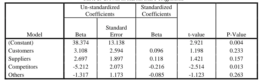
There was evidence that a relationship existed between market share of competitors and their market penetration, where (table 2): Growth in Market Share = 38.374 – 5.212 Competitors.

(0.004) (0.013)

Table 2: Growth in market share-coefficients

Dependent variable: GMS

There was evidence that objective forecasting technique was statistically significant, where (table 3): Ratio of forecast accuracy = 3.956 + 0.103 Objective method.

(0.000) (0.032)

Table 3: Forecasting methods – regression analysis coefficients

Table 20

Origin of Customers and Market Share - Coefficients

Model

Un-standardized Coefficients

Standardized Coefficients

t-Value P-Value Beta

Standard

Error Beta

1 (Constant) 32.866 11.209 2.932 0.004

Local -1.113 2.227 -0.036 -0.500 0.618

External 4.467 0.904 0.383 4.942 0.000

Mixed 0.756 1.202 0.059 0.629 0.530

Unique -1.229 1.117 -0.098 -1.100 0.273

Others -.341 1.499 -0.016 -0.227 0.820

Dependent variable: Market share

Table 3

Growth in Market Share – Coefficients

Model

t-value P-Value Beta

Standard

Error Beta

1 (Constant) 38.374 13.138 2.921 0.004

Customers 3.108 2.594 0.096 1.198 0.233

Suppliers 2.697 1.897 0.118 1.421 0.157

Competitors -5.212 2.073 -0.216 -2.514 0.013

Others -1.317 1.173 -0.085 -1.123 0.263

(10)

Dependent variable: Ratio of forecast accuracy

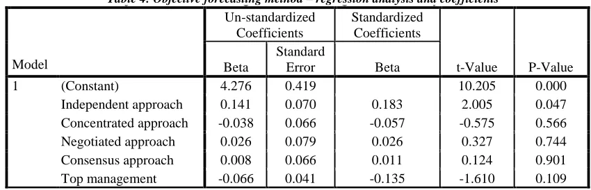
There was evidence that objective forecasting technique was statistically significant through the independent approach of forecasting, where (table 4):

Ratio of forecast accuracy = 4.276 + 0.141 Independent approach. (0.000) (0.047)

Table 4: Objective forecasting method – regression analysis and coefficients

Dependent variable: Ratio of forecast accuracy

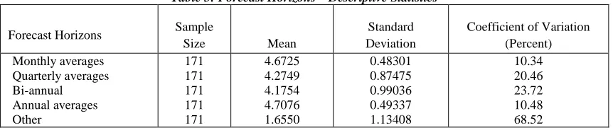
Due to their low standard deviation and variability, there was evidence that annual and monthly forecasts yielded APF (table 5).

Table 4

Forecasting Methods - Regression Analysis Coefficient

s

Model

Standard

Error Beta

1 (Constant) 3.956 0.328 12.078 0.000

Objective 0.103 0.048 0.167 2.156 0.032

Judgmental 0.077 0.048 0.133 1.596 0.112

Combination -0.006 0.057 -0.008 -0.101 0.920

Other 0.015 0.058 0.021 0.265 0.791

Dependent variable: Ratio of Forecast Accuracy

Table 5

Objective Forecasting Method – Regression Analysis, Coefficients

Model

Standard

Error Beta

1 (Constant) 4.276 0.419 10.205 0.000

Independent approach 0.141 0.070 0.183 2.005 0.047

Concentrated approach -0.038 0.066 -0.057 -0.575 0.566

Negotiated approach 0.026 0.079 0.026 0.327 0.744

Consensus approach 0.008 0.066 0.011 0.124 0.901

Top management -0.066 0.041 -0.135 -1.610 0.109

(11)

http: // www.gjesrm.com (C) Global Journal of Engineering Science and Research Management

Forecast Horizons Sample

Size Mean

Standard Deviation

Coefficient of Variation (Percent) Monthly averages Quarterly averages Bi-annual Annual averages Other 171 171 171 171 171 4.6725 4.2749 4.1754 4.7076 1.6550 0.48301 0.87475 0.99036 0.49337 1.13408 10.34 20.46 23.72 10.48 68.52

There was evidence that combined FT yielded higher APF through preparers’ knowledge and time horizons, where (table 6): Ratio of forecast accuracy = 0.172 Preparers’ knowledge - 0.138 Time horizon

(0.034) (0.036)

Table 6: Combined Forecasting Method - Regression Analysis, Coefficients

Model

Standard

Error Beta

1 (Constant) 1.342 0.723 1.855 0.065 Accuracy 0.183 0.112 0.136 1.630 0.105 Ease of use 0.097 0.146 0.080 0.665 0.507 Ease of interpretation 0.009 0.124 0.009 0.075 0.940 Preparers’ knowledge 0.172 0.080 0.220 2.143 0.034 Knowledge of users -0.058 0.069 -0.081 -0.851 0.396 Frequency of preparation 0.000 0.071 0.000 0.004 0.997 Time horizon -0.138 0.065 -0.220 -2.114 0.036 Software availability 0.064 0.067 0.085 0.962 0.338 Cost of forecasting 0.052 0.072 0.057 0.728 0.468 Timeliness 0.204 0.116 0.148 1.765 0.080 Data needs and sources 0.128 0.067 0.151 1.905 0.059

Dependent Variable: Ratio of Forecast Accuracy

(12)

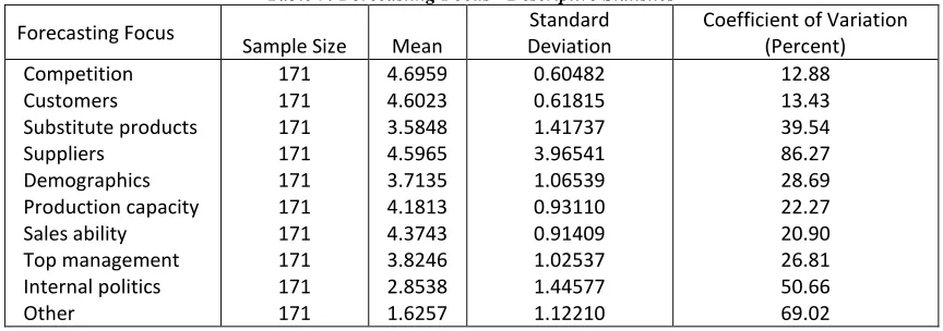
Table 7: Forecasting Focus - Descriptive Statistics

Forecasting Focus

Sample Size Mean

Standard Deviation

Coefficient of Variation (Percent) Competition Customers Substitute products Suppliers Demographics Production capacity Sales ability Top management Internal politics Other 171 171 171 171 171 171 171 171 171 171 4.6959 4.6023 3.5848 4.5965 3.7135 4.1813 4.3743 3.8246 2.8538 1.6257 0.60482 0.61815 1.41737 3.96541 1.06539 0.93110 0.91409 1.02537 1.44577 1.12210 12.88 13.43 39.54 86.27 28.69 22.27 20.90 26.81 50.66 69.02

There was evidence that judgmental FT was risky with high variability (table 8).

Table 8: Forecasting Methods – Descriptive Statistics

Forecast Methods Sample Size Mean Standard Deviation Coefficient of Variation (Percent)

Objective 171 3.9064 1.00733 25.79

Judgmental 171 3.6608 1.06916 29.21

Combination 171 3.8596 0.91597 23.73

Other 171 1.2865 0.83652 65.02

There was evidence that a FT influenced APF. The objective FT, through the independent approach, was superior, where (table 9): Ratio of forecast accuracy = 3.956 + 0.103 Objective method.

(13)

http: // www.gjesrm.com (C) Global Journal of Engineering Science and Research Management

Table 9: Forecasting Methods - Regression Analysis Coefficients

Model

Standard

Error Beta

1 (Constant) 3.956 0.328 12.078 0.000

Objective 0.103 0.048 0.167 2.156 0.032

Judgmental 0.077 0.048 0.133 1.596 0.112

Combination -0.006 0.057 -0.008 -0.101 0.920

Other 0.015 0.058 0.021 0.265 0.791

Dependent variable: Ratio of Forecast Accuracy

H1: There was evidence that EOE had an influence on the three FTs with all FTs having a partial influence on APF through EV and ROS (table 10-14).

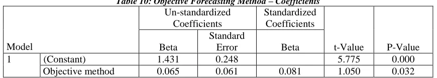
EV = 1.431 + 0.065 Objective FT. (0.000) (0.032)

Table 10: Objective Forecasting Method – Coefficients

Model

Standard

Error Beta

1 (Constant) 1.431 0.248 5.775 0.000

Objectivemethod 0.065 0.061 0.081 1.050 0.032

Dependent Variable: Expected Value (EV) ROS = 13.9914 - 0.994 Objective FT.

(0.000) (0.002)

Table 11: Objective Forecasting Method – Coefficients

Model Un-standardized

Coefficients

Standard

Error Beta

1 (Constant) 13.914 1.291 10.774 0.000

(14)

Dependent Variable: ROS

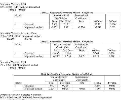
EV = 2.308 - 0.171 Judgmental method (0.000) (0.003)

Table 12: Judgmental Forecasting Method – Coefficients

Coefficients

t-Value P-Value Beta Std. Error Beta

1 (Constant) 2.308 .216 10.701 0.000

Judgmental method -0.171 .057 -0.226 -3.019 0.003

Dependent Variable: Expected Value ROS = 9.093 + 0.256 Judgmental method (0.000) (0.010)

Table 13: Judgmental Forecasting Method – Coefficients

Coefficients

1 (Constant) 9.093 1.180 7.705 0.000

Judgmental method 0.256 0.310 0.063 0.826 0.010

EV = 1.970 - 0.074 Combined method (0.000) (0.002)

Table 14: Combined Forecasting Method – Coefficients

Model

t-Value P-Value

Beta Std. Error Beta

1 (Constant) 1.970 0.268 7.354 0.000

Combined method -0.074 0.068 -0.084 -1.101 0.002

Dependent Variable: Expected Value (EV)

ROS = 9.307 + 0.187 Combined forecasting method (0.000) (0.005)

H2: There was no evidence that IOE had an influence on APF.

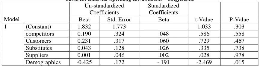
H3: There was evidence that EOE partially influenced APF through ROA under demographic characteristics, where (table 15): ROA = -0.425 Demographic characteristics

(15)

http: // www.gjesrm.com (C) Global Journal of Engineering Science and Research Management

Model

t-Value P-Value

1 (Constant) 1.832 1.773 1.033 .303

competitors 0.190 .324 .048 .586 .558

Customers 0.231 .317 .060 .729 .467

Substitutes 0.043 .128 .026 .335 .738

Suppliers 0.001 .046 .002 .028 .978

Demographics -0.425 .172 -.191 -2.469 .015

Dependent Variable: ROA

H4: There was evidence that EOE had a partial moderating effect on the relationship between objective FT and APF through ROS and ROA, where (tables 16 and 17):

ROS = 11.986 – 1.070 Objective method (0.001) (0.002)

Table 16: External Operating Environment – Coefficients

Model

1 (Constant) 11.986 3.422 3.502 0.001

Competitors 0.622 0.583 0.087 1.067 0.288

Customers -0.233 0.573 -0.033 -.407 0.684

Substitutes 0.059 0.231 0.019 0.256 0.798

Suppliers -0.086 0.084 -0.079 -1.021 0.309

Demographics 0.150 0.321 0.037 0.468 0.640

Objective method

-1.070 0.337 -0.250 -3.176 0.002

(16)

Model

1 (Constant) 1.702 1.905 0.894 0.373

Competitors 0.189 0.325 0.048 0.583 0.561

Customers 0.235 0.319 0.061 0.738 0.462

Substitutes 0.043 0.129 0.026 0.334 0.739

Suppliers 0.003 0.047 0.005 0.059 0.953

Demographics -0.434 0.178 -0.195 -2.430 0.016

Objective method 0.036 0.188 0.015 0.190 0.850

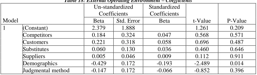
There was evidence that EOE had a partial moderating effect on the relationship between judgmental FT and APF through ROA, where (table 18):

ROA = - 0.429 Demographics (0.014)

Model

1 (Constant) 2.379 1.888 1.261 0.209

Competitors 0.184 0.324 0.047 0.568 0.571

Customers 0.221 0.318 0.058 0.696 0.487

Substitutes 0.060 0.130 0.036 0.460 0.646

Suppliers 0.005 0.046 0.009 0.112 0.911

Demographics -0.429 0.172 -0.193 -2.489 0.014

Judgmental method -0.147 0.172 -0.066 -0.852 0.396

There was evidence that EOE had a partial moderating effect on the relationship between combined FT and APF through ROA under demographic characteristics, (table 19):

(17)

http: // www.gjesrm.com (C) Global Journal of Engineering Science and Research Management

Model

1 (Constant) 1.270 1.965 0.646 0.519

Competitors 0.187 0.324 0.048 0.578 0.564

Customers 0.248 0.319 0.065 0.778 0.438

Substitutes 0.041 0.129 0.025 0.319 0.750

Suppliers 0.000 0.046 0.001 0.008 0.994

Demographics -0.426 0.172 -0.191 -2.469 0.015

Combined method 0.133 0.198 0.051 0.669 0.504

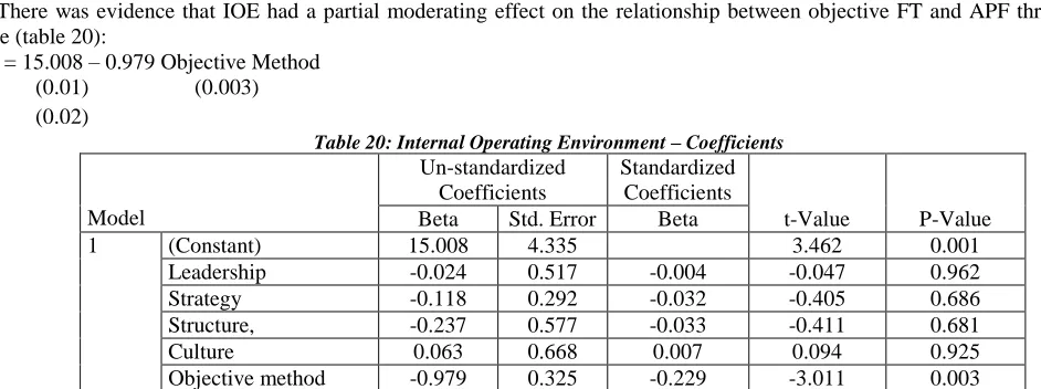
H5: There was evidence that IOE had a partial moderating effect on the relationship between objective FT and APF through ROS, where (table 20):

ROS = 15.008 – 0.979 Objective Method

(0.01) (0.003)

(0.02)

Table 20: Internal Operating Environment – Coefficients

Model

1 (Constant) 15.008 4.335 3.462 0.001

Leadership -0.024 0.517 -0.004 -0.047 0.962

Strategy -0.118 0.292 -0.032 -0.405 0.686

Structure, -0.237 0.577 -0.033 -0.411 0.681

Culture 0.063 0.668 0.007 0.094 0.925

Objective method -0.979 0.325 -0.229 -3.011 0.003

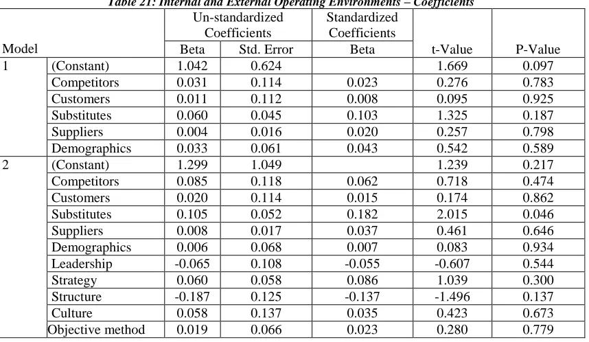
H6: There was evidence that the joint effect of internal and external OEs had a partial moderating effect on the relationship between objective FT and APF through EV and ROS, where (table 21):

(18)

Table 21: Internal and External Operating Environments – Coefficients

Model

t-Value P-Value

1 (Constant) 1.042 0.624 1.669 0.097

Competitors 0.031 0.114 0.023 0.276 0.783

Customers 0.011 0.112 0.008 0.095 0.925

Substitutes 0.060 0.045 0.103 1.325 0.187

Suppliers 0.004 0.016 0.020 0.257 0.798

Demographics 0.033 0.061 0.043 0.542 0.589

2 (Constant) 1.299 1.049 1.239 0.217

Competitors 0.085 0.118 0.062 0.718 0.474

Customers 0.020 0.114 0.015 0.174 0.862

Substitutes 0.105 0.052 0.182 2.015 0.046

Suppliers 0.008 0.017 0.037 0.461 0.646

Demographics 0.006 0.068 0.007 0.083 0.934

Leadership -0.065 0.108 -0.055 -0.607 0.544

Strategy 0.060 0.058 0.086 1.039 0.300

Structure -0.187 0.125 -0.137 -1.496 0.137

Culture 0.058 0.137 0.035 0.423 0.673

Objective method 0.019 0.066 0.023 0.280 0.779

Dependent Variable: Expected value ROS = 14.857 – 1.055 Objective FT

(0.007) (0.002)

There was evidence that the joint effect of internal and external OEs had a partial moderating effect on the relationship between combined FT and APF through EV under substitute products, where (table 22):

(19)

http: // www.gjesrm.com (C) Global Journal of Engineering Science and Research Management

Model

t-Value P-Value

1 (Constant) 1.042 0.624 1.669 0.097

Competitors 0.031 0.114 0.023 0.276 0.783

Customers 0.011 0.112 0.008 0.095 0.925

Substitutes 0.060 0.045 0.103 1.325 0.187

Suppliers 0.004 0.016 0.020 0.257 0.798

demographics 0.033 0.061 0.043 0.542 0.589

2 (Constant) 1.436 1.040 1.381 0.169

Competitors 0.083 0.118 0.061 0.705 0.482

Customers 0.015 0.114 0.011 0.128 0.898

Substitutes 0.104 0.052 0.179 1.977 0.050

Suppliers 0.007 0.016 0.034 0.434 0.665

demographics 0.010 0.066 0.013 0.152 0.880

Leadership -0.063 0.107 -0.052 -0.583 0.561

Strategy 0.059 0.058 0.083 1.006 0.316

Structure -0.181 0.126 -0.133 -1.440 0.152

Culture 0.066 0.139 0.040 0.476 0.634

Combined method -0.030 0.072 -0.033 -0.410 0.683

Dependent Variable: Expected value (EV)

Discussion Of results

Comparison of forecasting methods in accuracy of performance forecasting

Using EV, ROS, ROA and GMS as indicators of APF, study results for this objective indicated that objective, judgmental and combined FTs achieved APF through EV and ROS. These findings indicated that in order to assess the accuracy of a FT, relevant independent variables of the OE and dependent variables of APF need to be fully and appropriately identified. It is likely that ROA is limited to a firm’s bottom line rather than being considered within the boundary limits of EV. On the other hand, the evaluation of GMS could relate only to sales volume without considering reduction in prices. These two APF indicators appeared to be irrelevant in assessing which FT was superior.

Identification of performance measures influenced by the OE

(20)

Assessment of moderating effect of EOE on the relationship between a FT and APF

Results indicated that the EOE had a moderating effect as follows: For the objective method, ROS and ROA were statistically significant. For the judgmental and combined methods, ROA was statistically significant. This implied that the EOE had a moderating effect on the relationship between a FT and APF. On the other hand, the IOE did not have a significant moderating effect on the relationship between a FT and APF apart from ROS with regard to the objective forecasting method.

Examination of relationships among FTs, OE and APF

Results indicated that the joint effect of the OEs had a moderating effect between the objective method and APF through EV and ROS, and combined method through EV only. The OEs had no moderating effect on the relationship between judgmental method and APF. This implied that the IOE is possibly well managed in LFMs. The study showed that the objective FT was more superior to either the judgmental or combined FTs. Simple averaging of judgmental and objective forecasts without considering the effects of the OE resulted in a combined FT that was statistically not significant, and ignoring the effects of the OE would render a FT inaccurate.

Conclusions

The main purpose of this research study was to assess FTs, OE and APF in LMFs in Kenya. Findings indicate that a forecasting strategy must be well articulated to take into account factors of the operating environment in order to manage the dynamic and turbulent changes within the OE. The management of customers, suppliers and the effect of substitute products and demographic characteristics were found to be key variables in the EOE affecting APF. The objective forecasting technique was found to be superior followed by combined forecasting, while judgmental method was statistically not significant. Secondly, in each of the three FTs, ROS and ROA were influenced by the internal and external OEs separately, while the joint effect of the OEs had a moderating effect on the relationship between combined FT and APF. Additionally, the joint effect of the OEs had a moderating effect on the relationship between objective FT and ROS plus ROA. Consequently, the accuracy of a FT depends on both the nature and significance of the independent and joint effects of the OEs on business indicators.

Thirdly, the adoption of combined FT could result in higher APF, but the use of this technique requires resources with relevant skills, acquisition of appropriate software and adequate funding of the forecasting establishments as LMFs in Kenya face the challenges of understanding the greater complexity and risks inherent in the global environment. The design and management of forecasting activities must consider the intense market rivalry and differences in culture and sectoral structures of an industry. A much broader set of skills and professionalism are required to implement the objective and combined forecasting techniques; compatibility of information technologies and standardization of systems and data are crucial to a firm’s ability to integrate forecasting operations on a broader basis; and decision support tools that incorporate internal and external environmental variables and allow “what if” scenario analysis are important to enable managers to effectively manage the complexities and uncertainties of the OE.

References

1. Abor, J., and Quartey, P. (2010): “Issues in SME Development in Ghana and South”. University of Ghana Business School, Legon.

2. Ackhoff, R. (1981): “Creating the Corporate Future: Plan or be Planned for”. New York: Wiley.

(21)

http: // www.gjesrm.com (C) Global Journal of Engineering Science and Research Management

4. Augustine, B., Bhasi, M. and Madhu, G. (2012), “Linking SME Performance with the Use of Forecasting Planning and Control”: Empirical Findings from the India Firms

5. Annastiina, K., Jukka, K. and Janne, H. (2009), “Demand Forecasting Errors in Industrial Context: Measurements and Impacts”, International Journal of Production Economics, Vol. 118, pp. 43-48.

6. Armstrong, J. S. (2001). “Evaluating Forecasting Methods”. Principles of Forecasting: A Handbook for Researchers and Practitioners.

7. Aviv, Y. (2003): “A Time Series Framework for Supply Chain Inventory Management”.

8. Aviv, Y. (2007): “Benefits of Collaborative Forecasting Partnership Between Retailers and Manufacturers”.

9. Berg J., Nelson F., and Rietz, T. (2003): “Accuracy and Forecast Standard Error of Prediction Markets”. Department of Accounting, Economics and Finance, Henry B. Tippie College of Business Administration, University of Iowa.

10. Bolo, A. Z. (2007): “The Effect of Selecting Strategy Variables on Corporate Performance”: A Survey of Supply Chain Management in Large Private Manufacturing Firms in Kenya. Unpublished PhD Thesis, University of Nairobi.

11. Brownlees, C. T., and Gallo, G. M. (2007): “Volatility Forecasting Using Explanatory Variables and Focused Selection Criteria”.

12. Bunn, D. W., and Taylor, J. W. (2001): “Setting Accuracy Targets for Short-Term Judgmental Sales Forecasting”. International Journal of Forecasting (2001), pp. 159-169.

13. Bunn, D. W., and Taylor, J. W. (2001): “Review of Practical Guidelines for Combining Forecasts”. 14. Castillo, J. J., (2009): “Stratified Sampling Method”.

15. Chann, K. K. (2000): “Forecasting Demand and Inventory Management Using Bayesian Systems”, Vol. 11, pp. 331 – 339. 16. Clemen, R. T., and Murphy, A. H. (1986a, b): “Combining Forecasts”: A Review and Annotated Bibliography. University of

Oregon.

17. Davis, D. F., and Mentzer, J. T. (2007): “Organizational Factors in Sales Forecasting Management”: International Journal of Forecasting (2007) pp. 475-495.

18. Fader, P. S., Hardie, B. G. S., and Huang, C. (2004). “A Dynamic Changepoint Model for New Product Sales Forecasting”. Marketing Science. Vol. 23, No. 1, Winter 2004, pp. 50-56.

19. Fildes, R. (2006): “An Evaluation of Bayesian Forecasting”.

20. Fildes, R., and Makridakis (1995): “The Impact of Empirical Accuracy Studies on Time Series Analysis and Forecasting”. International Statistical Review, Vol. 63, No. 3, (Dec., 1995), pp. 289 – 308.

21. Fok, D., and Franses, H. P. (2001): “Forecasting Market Shares from Models for Sales”. 22. International Journal of Forecasting 17 (2001) pp. 121-128.

23. Frees, E. W., and Miller, T. W. (2004). “Sales Forecasting Using Longitudinal Data Models”. International Journal of Forecasting 20 (2004) pp. 99-114.

24. Foslund, and Jonsson (2007): “User Influence on the Relationship Between Forecasts”.

25. Gardner, E. S. et al. (2001). “Further Results on Focus Forecasting Versus Exponential Smoothing”. International Journal of Forecasting 17 (2001) pp. 287-293.

26. Ghodrati, B., and Kumar, D. (2005): “Reliability and Operating Environment Based Spare Parts Planning”. 27. Heizer, J. H., and Render, B. (1991): “Evaluation of Forecasting Methods”.

28. Hendry, D. F., and Clements, M. P. (2002): “Combining Forecasts”.

(22)

30. Hyndman, J., and Koehler, A. (2005): “Another Look at Measures of Forecast Accuracy”. Department of Decision-Making Science and Management Information Systems, Miami University. USA.

31. Intriligator, M. D. (2001): “The Econometrics of Macroeconomic Forecasting”. Economic Journal. 32. Johnston K. (1975): “Consumer Demand Theory”.

33. Karami, A., Analoui, F. and Kakabadse, N. K. (2006), “The CEOs Characteristics and Strategy Development in UK SME Sector”, Journal of Management Development, Vol. 25 No.4, pp. 316-324.

34. Kate, C. (2006). “Statistical Methods and Computing: Sample Size for Confidence Intervals with Known t Intervals”. 374 SH, ISBN. 335-0727. UIOWA

35. Khandwalla, P. N. (1977): “Management Styles and Organizational Effectiveness”.

36. Kibera, F. N. (1996). “Introduction to Business: A Kenyan Perspective”. Nairobi, Kenya Literature Bureau.

37. Larrick, R. P., and Soll, J. B. (2003): “To Combine or Not to Combine: Selecting Among Forecasts and Their Combinations”. 38. Lawrence, J. C. (1983): “An Extrapolation of Some Practical Issues in the Use of Quantitative Forecasting Models”. Journal

of Forecasting, Vol. 2 pp. 169-179.

39. Lawrence, M., and O’Connor, M. (2000): “Sales Forecasting Updates: How Good are they in Practice”? International Journal of Forecasting 16 (2000) pp. 369-382.

40. Lawrence, M. J., Edmundson, R. H., and O’Connor, M. J. (1986): “The Accuracy of Combining Judgemental and Statistical Forecasts”. Management Science. Vol. 32, No.12 (December 1986), pp. 1521–1532.

41. Lindblom, A. T. et al (2008). “Market-Sensing Capability and Business Performance of Retail Entrepreneurs”. Contemporary Management Research.

42. Makridakis, S., and Winkler, R. L. (1983) 146, Part 2, pp. 150 - 157: “The Combination of Forecasts”. Indiana University, USA; Insead, Fontainebleau, France.

43. Makridakis, S., and Hibon, M. (2000): “Time Series Forecasting Competition; and Artificial Neural Network and Computational Intelligence Forecasting Competition”.

44. McCarthy, T. M., et al. (2006): “The Evolution of Forecast Management: A Survey of Forecasting Executives”.

45. Mbeche, I. M., and Yego, D. K. S.: “A Survey of the Application of Forecasting Methods in Large Manufacturing Firms in Nairobi, Kenya”. Nairobi Journal of Management Vol.2, October1996.

46. Mentzer, J. T, Bienstock, C. C., and Kahn, K. B. (1998): “Benchmarking Sales Forecasting Management”. Business Horizons, November-December 1998.

47. Mentzer, J. T., and Kahn, K. B. (1997): The State of Sales Forecasting Systems in Corporate America.

48. Moon, M. A., Mentzer, J. T., and Smith, C. D (2003). “Conducting a Sales Forecasting Audit”. International Journal of Forecasting 19 (2003) pp. 5-2Moorman, C., Zaltman, G., and Deshpande, R. (1992). “Relationships between Providers and Users of Market Research: The Dynamic of Trust within and Between Organizations”. Journal of Marketing Research, 29, pp. 314-328.

49. Nachiappan, S. P. (2005): “Performance Analysis of Forecast Driven Vendor Managed Inventory”. 50. Newbold, P., and Harvey, I. H. (2002): “Combination of Forecast Methods”.

51. Nyanamba, N. (2003): “A Methodology for Forecasting Sales Demand for Tooth Paste: The Case of Colgate Palmolive (EA) Limited”. Unpublished MBA Project,

University of Nairobi.

52. Reeves, R. J. E. (1992): “Design-based Research in Education”.

(23)

http: // www.gjesrm.com (C) Global Journal of Engineering Science and Research Management

Application and Logistics Performance”.

54. Stanley, E. G. and Gregory, M. M., (2001): “Achieving World Class Supply Chain Alignment: Benefits, Barriers and Bridges”. A Compiled Research Report.

55. Synader, T. (2008): “Rational Sales Forecasting: The Convergence of Skills, Strategy and Pipeline Management”.

56. Timmermann, A. (2006): “Forecast Combinations”. A Handbook of Economic Forecasting, Elsevier Science B.V.

57. Turgut, K. (2007): “The Use of Encompassing Tests for Forecast Combinations”. IMF Working Paper.

58. Vieira, G. E., and Favaretto, F. (2006): “A New and Practical Heuristic for Master Production Scheduling Creation”. International Journal of Production

Management, Vol. 44, Nos.18- 19, 15 September 1 October 2006, pp. 3607-3625. 59. Vorhies, D. W., and Morgan, N. A. (2005). “Benchmarking Marketing Capabilities for Sustainable Competitive Advantage”. Journal of Marketing, 69(1), pp. 80-94.

60. Waweru M. A. S (2008): “Competitive Strategy Implementation and Its Effect on Performance in Large Private Sector Firms in Kenya”. Unpublished PhD Thesis, University of Nairobi.

61. Winklhofer, H., Diamantopoulos, and Witt, S. F. (1996). “Forecasting Practice: A Review of the Empirical Literature and an Agenda for Future Research”.

International Journal of Forecasting 12 (1996), pp. 193-221

62. Whybark, D. C., Flores, and Benito (1986). “A Comparison of Focus Forecasting with Averaging and Exponential Smoothing”. Production and Inventory Management: The Journal of the American Production and Inventory Control Society, Vol. 27, pp. 96 -103 (1986).