Clustering with Hidden Markov Model on Variable Blocks

Clustering with Hidden Markov Model on Variable Blocks

Lin Lin llin@psu.edu

Jia Li jiali@psu.edu

Department of Statistics Pennsylvanian State University University Park, PA 16802, USA

Editor:Saharon Rosset

Abstract

Large-scale data containing multiple important rare clusters, even at moderately high dimensions, pose challenges for existing clustering methods. To address this issue, we propose a new mixture model called Hidden Markov Model on Variable Blocks (HMM-VB) and a new mode search algorithm called Modal Baum-Welch (MBW) for mode-association clustering. HMM-VB leverages prior information about chain-like dependence among groups of variables to achieve the effect of dimension reduction. In case such a dependence structure is unknown or assumed merely for the sake of parsimonious modeling, we develop a recursive search algorithm based on BIC to optimize the formation of ordered variable blocks. The MBW algorithm ensures the feasibility of clustering via mode association, achieving linear complexity in terms of the number of variable blocks despite the exponentially growing number of possible state sequences in HMM-VB. In addition, we provide theoretical investigations about the identifiability of HMM-VB as well as the consistency of our approach to search for the block partition of variables in a special case. Experiments on simulated and real data show that our proposed method outperforms other widely used methods. Keywords: Gaussian mixture model, hidden Markov model, modal Baum-Welch algorithm, modal clustering

1. Introduction

Clustering is one of the most important topics in unsupervised learning, the goal of which is to discover structures from a collection of unlabeled data. Finite mixture modeling is a major statistical framework for clustering. Without attempting to review its expansive applications, we offer instead a few examples as a glimpse at the incredibly broad usage of mixture modeling (Escobar and West (1995); Allenby et al. (1998); McLachlan et al. (2002); Kasahara and Shimotsu (2009)).

One important advantage of the mixture model is that the goodness of fit to any data can be improved by increasing the number of mixture components. The simplest approach to clustering based on a mixture model is to assign each component to an individual cluster. However, there are several drawbacks to equate clusters with mixture components, among which is that the parametric distribution of a component is too restrictive for the potentially diverse shapes of clusters (see Li et al. (2007) for a thorough discussion). Various strategies have been proposed to merge multiple mixture components so that an individual cluster can be more properly modeled (Hennig, 2010; Li, 2005; Pyne et al., 2009; Finak et al.,

c

2009; Chan et al., 2010; Aghaeepour et al., 2011; Lin et al., 2016; Melnykov, 2016). In the statistical learning literature, a prominent method for merging multiple mixture components into one cluster is based on the modes of the mixture density, the so-called modal clustering by Li et al. (2007). We discuss this method in more detail in Section 2.

Despite their wide applications, existing mixture modeling approaches are severely challenged by high dimensional data encountered in certain research areas, for example, cell subset identification using data generated by the high-throughput single-cell technolo-gies (Perfetto et al., 2004; Bandura et al., 2009; Maecker et al., 2012; Chattopadhyay et al., 2014; Spitzer and Nolan, 2016). These data sets contain a large number of highly unbalanced clusters. Furthermore, the most interesting clusters for scientific investigation are often of remarkably low occurrence. Even when the data dimension is not impressively large by today’s standard, say in the order of tens, existing methods have much difficulty for detecting clusters of very low probabilities. Low probability mixture components tend to be “concealed” by large background clusters in the data. For the usual mixture modeling approach, in order to capture the rare clusters, we must increase the number of components dramatically. On the other hand, the curse of dimensionality prevents the use of many components; the growing computational intensity is also a concern.

Our new method is motivated by the popular manual gating analysis of single-cell cytometry data (details in Section 5.2), in which the variables are divided into groups based on prior information and examined sequentially. The key idea here is to exploit the chain-like dependence among groups of variables in the construction of a mixture model. Lin et al. (2013) used this idea to build a relatively primitive model. In this approach, the variables

are partitioned into two groups, and the mixture model is estimated using the hierarchical Dirichlet process prior. This two-block model is substantially more efficient and accurate in rare clusters identification than the conventional mixture models are. The existing method, however, is unable to move beyond two variable blocks in practice due to the exponential computational complexity. The Markov chain Monte Carlo (MCMC) simulation for the two-block model is already highly intensive and is coupled by the long-standing issue of label switching when MCMC is applied to estimate mixture models (e.g., Richardson and Green (1997); Celeux et al. (2000); Stephens (2000)).

The aim of this paper is to design an effective and computationally accessible statistical model that can fit data robustly in both high and low probability regions and can identify clusters of non-Gaussian shapes. We propose a new model to exploit sequential dependence among variable groups. We also develop an algorithm to search for such a dependence structure when it is unknown. Our experiments show that even if the sequential dependence is not backed up by domain knowledge, it can still be useful as a mathematical mechanism for parsimonious modeling.

develop theorems on the identifiability of HMM-VB given the variable block structure and the identifiability of the variable blocks under certain conditions. We prove the consistency of the BIC criterion for finding the variable blocks in a special case.

The rest of the paper is organized as follows. In Section 2, we introduce notations and overview existing techniques most relevant to our proposed methods. In Section 3, we present HMM-VB and efficient algorithms for model fitting and modal clustering. In Section 4, we provide theoretical results on identifiability, consistency, and the mode search algorithm for HMM-VB. Proofs of the theorems appear in Appendix B∼D. In Section 5, experimental results are reported for both simulated and real data including mass cytometry, single-cell genomics, and image data. Comparisons are made with some competing models and popular methods. We conclude with discussions in Section 6.

2. Preliminaries

Given a random vector X= (X1, X2, ..., Xd)0 ∈ Rd, letxi = (xi1, ..., xid)0 ∈ Rd be thei-th

sample of X, wherei= 1, ..., n. Denote by X= (x1,x2, ...,xn)∈ Rn×d the data matrix, and

we let Xj be the j-th column of X which contains the values ofXj across all the sample points. For ease of notation, we let x∈ Rd_{be a realization of the random vectorX.}

The finite Gaussian mixture model (GMM) is commonly used for clustering. A GMM with M components has the density function: f(x|θ) = PM

k=1 πkφ(x|θk) , where πk is

the mixture component prior probability and φ(· |θk) is the multivariate normal density parameterized by θk = (µk,Σk), µk being the d-dimensional mean vector and Σk the d×d covariance matrix. For model estimation, a latent indicator Z ∈ {1,2, ..., M} with

P(Z =k) =πk is used. Specifically, conditioning on Z =k,X follows the k-th component distribution. Z is also called the component identity ofX. To perform clustering, the usual approach is to compute the posterior probability P(Z = k|X = x) and assign x to the cluster with the maximum posterior. However, this approach is inadequate to model clusters with arbitrary shapes and cannot ensure that the clusters are reasonably separated. One major idea explored in the literature is to merge multiple mixture components for a better and more flexible representation of an individual cluster. We refer to Melnykov and Maitra (2010) for a thorough review on clustering based on finite mixture models.

Banfield and Raftery (1993) and Celeux and Govaert (1995) propose to decompose the covariance matrix of the mixture components in a GMM into parts that control volume, shape, and orientation respectively and allow model constraints to be imposed in these aspects either individually or by combination. A model selection criterion is then used to choose a GMM in terms of not only the number of components but also the constraints on covariance matrices. A popular R package, namelyMclust(Fraley and Raftery, 2006), is implemented for this method, which we will use for comparison.

The Modal EM (MEM) algorithm developed by Li et al. (2007) performs efficient merging of mixture components. It resembles the expectation-maximization (EM) algorithm (Demp-ster et al., 1977), as reflected by the name “modal EM”. However, the objective of MEM is to find an increasing path from any data point to a local maximum of a given density. Hence, the optimization objective of MEM is to find a local maximizer overx forf(x|θ) under a given

θ, while EM is to find local maxima over θforf(x|θ) given x. Consider a general mixture density f(x) =PM

Starting from any initial value denoted byx[0], MEM solves a local maximum of the mixture density by the following two iterative steps: (1) At iteration r, let pk = πkfk(x

[r]₎

f(x[r]₎ ,k = 1,

..., M; (2) Update x[r+1] _{= argmax}

x

PM

k=1pklogfk(x). MEM stops when a pre-specified

stopping criterion is met. Specifically for GMM with f(x) = PM

k=1πkφ(x|µk,Σk), MEM

becomes

1. E-step: Solve

pk= πkφk(x

[r]_|µk,Σ

k)

f(x[r]₎ , k= 1, ..., M. (1)

2. M-step: Solve

x[r+1]=

M

X

k=1

pk·Σ−k1

!−1 ·

M

X

k=1

pk·Σ−k1µk

!

. (2)

The computational efficiency of MEM enabled the development of a new clustering approach by Li et al. (2007), referred to as modal clustering. In Li et al. (2007), a non-parametric Gaussian kernel density estimate is used, and MEM is applied to find the mode associated with every point. Data points associated with the same mode are assigned to the same cluster. In Lee and Li (2012), modal clustering based on the general finite GMM is studied. For computational efficiency, instead of applying MEM to every data point, it is applied to the means of the mixture components. Components with mean vectors associated with the same mode are merged into one cluster. Whether a point-wise mode association or a component-wise mode association is preferred depends on the nature of the application and the computational resources. In practice, the difference in the clustering results we have observed is quite small. We refer to the clustering method based on component-wise mode association asmodal GMM and use it as a baseline for comparison with our new method.

Under the framework of modal clustering, the purpose of a mixture component is primarily for good density estimation. We no longer rely on a one-to-one correspondence between mixture components and clusters. Mode association also ensures that different clusters of data are well separated. See Li et al. (2007) for more detailed discussion on these advantages. The flexibility provided by modal clustering for fitting data is precisely what we need for the applications we consider. In the next section, we propose a HMM-type model which can be cast as a mixture model with an enormous number of components, even exceeding the data size. This complexity causes no difficulty in clustering via mode association.

3. Hidden Markov Model on Variable Blocks

mixture component identities). The description of a conventional HMM is provided in Appendix A. We call our new model Hidden Markov Model on Variable Blocks (HMM-VB). Suppose the d-dimensional random vector X is partitioned into T blocks indexed by

t= 1,2, ..., T. Let the number of variables in blocktbedt, wherePTt=1dt=d. Assume that

thed1variables in block 1 have indices before thed2variables in block 2, and so on. In general, obviously, such an ordering of variables may not hold. But this is only a matter of naming the variables and has no effect on our results. LetX(t) denote thet-th variable block. Without loss of generality, let X(1) = (X1, X2, ..., Xd1)

0 _{and X}(t) _{= (Xm}

t+1, Xmt+2, ..., Xmt+dt) 0_, where mt=Pt−1

τ=1dτ, fort= 2, ..., T.

Denote the underlying state of X(t) as st, t = 1, ..., T. Let the index set of st be

St={1,2, ..., Mt}, whereMt is the number of mixture components for variable blockX(t), t= 1, ..., T. Let the set of all possible sequences be ˆS =S1× S2· · · × ST. |S|ˆ=

QT

t=1Mt. We assume:

1. {s1, s2, ..., sT}follow a Markov chain. Let πk =P(s1=k),k∈ S1. Let the transition probability matrix At = (a(_k,lt)) between st and st+1 be defined by a(_k,lt) = P(st+1 =

l|st=k),k∈ St,l∈ St+1.

2. Given st, X(t) is conditionally independent from other st0 and X(t 0₎

, for all t0 6= t. We also assume that given st = k, the conditional density of X(t) is the Gaussian

distributionφ(X(t)_|µ(t)

k ,Σ

(t)

k ).

Let s={s1, ..., sT}. A realization ofX isx, and a realization of X(t) isx(t). To summarize, the density of HMM-VB is given by

f(x) =X

s∈Sˆ

πs1

T−1

Y

t=1

a(_st_t)_,st+1

!

·

T

Y

t=1

φ(x(t)|µ_s(t_t),Σ(_st_t)). (3)

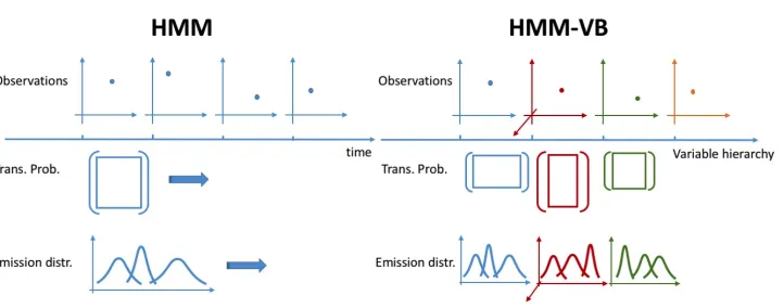
Remark 1: Figure 1 illustrates two major differences between HMM-VB and the conventional HMM. (1) The variable blocks X(t)_{’s are not from the same vector space. Hence, the} parameters of the distribution ofX(t) givenst=k depend not only on kbut also on t; (2) The underlying Markov chain for {s1, ..., sT}is not time invariant. In fact, the state space

S_t varies witht.

Remark 2: Although the density function of HMM-VB in Eq. (3) indicates block diagonal covariance matrices, there are important differences from a typical GMM with the same constraint on the covariance. First, the Gaussian mean vectors in Eq. (3) reside on a lattice in the Cartesian product spaceRd1_{× R}d2_{· · · × R}dT_{. Secondly, the number of components} grows exponentially with T. In fact, it is often larger than the sample size. The enormous number of components cannot be handled by a typical covariance constrained GMM from either estimation or computational feasibility perspectives.

Figure 1: Comparison between HMM-VB and HMM models. The observations under HMM have to be of a fixed dimension, 2 in this illustration. Typically, only one transition probability matrix is applied through time, and the set of distributions conditioned on the states at any time spot is also fixed. HMM-VB models data across blocks of different variables, possibly of different dimensions. Both the transition probability matrix and the set of conditional distributions are defined individually at every “time” spot.

3.1 Maximum Likelihood Estimation

HMM is usually estimated by the EM algorithm. However, because the cardinality of ¯S

grows exponentially with the sequence length, the computational complexity of a direct application of EM is of exponential complexity. This technical hurdle was overcome by the

Baum-Welch (BW) algorithm which achieves complexity of linear order in the sequence length and quadratic in the number of states without compromising optimality. The BW algorithm, a special instance of EM, was developed in the 1960’s before the general EM algorithm was developed in the 1970’s. As a result, we still call the estimation algorithm Baum-Welch, following the convention of the literature on HMM. We present the BW algorithm for HMM model estimation in Appendix A. For a detailed exposure to HMM, we refer to Young et al. (1997).

We now present the corresponding BW algorithm for HMM-VB. It can be proved that the BW algorithm for HMM is an exact EM algorithm. The derivation of the BW algorithm for HMM-VB is similar to the derivation of BW for the usual HMM. We thus omit it here. Clearly, it is not meaningful to estimate HMM-VB using a single sequence, which is essentially a single data point in this case. HMM-VB is after all a model for X∈ Rd_.

Denote by xi = (x(1)i , x

(2)

i , ..., x

(T)

i )0 the ordered and grouped i-th sample according

to the given variable blocks. We denote the original i-th sample before ordering by ˘xi.

Consider estimation of HMM-VB based on a data set{x1,x2, ...,xn}. We defineLk(xi, t)

and Hk,l(xi, t) similarly as in Eq. (8) and Eq. (9) in Appendix A. For i= 1, ..., n,

Lk(xi, t) = P(si,t=k|xi), k ∈ St, (4)

The BW algorithm iterates the following two steps:

1. E-step: Under the current set of parameters, compute Lk(xi, t), i= 1, ..., n, k∈ St, t= 1, ..., T, and Hk,l(xi, t),i= 1, ..., n,k∈ St,l∈ St+1,t= 1, ..., T−1.

2. M-step: Update parameters by

µ(_kt) =

Pn

i=1Lk(xi, t)x(it)

Pn

i=1Lk(xi, t)

, k∈ St, t= 1, ..., T,

Σ(_kt)=

Pn

i=1Lk(xi, t)

x(_it)−µ(_kt) x(_it)−µ(_kt)

0

Pn

i=1Lk(xi, t)

, k∈ St, t= 1, ..., T,

a(_k,lt) =

Pn

i=1Hk,l(xi, t)

Pn

i=1Lk(xi, t)

, k∈ S_t, l∈ S_t+1, t= 1, ..., T −1,

πk∝

n

X

i=1

Lk(xi,1), k∈ S1, s.t.

X

k∈S1

πk= 1.

The above equations can be easily extended to the case of weighted sample points. It can occur in practice that each sample point is assigned with a weight. For instance, quantization is often used to reduce the data size significantly. Instead of using the original data, one may use the quantized points, each of which can represent a different number of original points and hence is assigned with a weight proportional to that number. Suppose weightwi

is assigned to samplexi. The E-step is not affected. In the M-step, we can simply multiply wi in front of each summand appeared in the equations above.

The forward-backward algorithm for computing Lk(xi, t) and Hk,l(xi, t) is essentially the same as the forward-backward algorithm for the usual HMM. The fact that the variable blocks are not from the same vector space and the state spaces vary withtdoes not cause any intrinsic difference. Suppress the sample indexiand consider one sample point x.

Define the forward probability αk(x, t) as the joint probability of observing the firstt

variable blocksx(τ),τ = 1, ..., t, and being in statekat time t:

αk(x, t) =P(x(1), x(2), ..., x(t), st=k), k∈ St.

This probability can be evaluated by the following recursive formula:

αk(x,1) = πkφ(x(1)|µ(1)_k ,Σ(1)_k ), k∈ S1,

αk(x, t) = φ(x(t) |µ(_kt),Σ(_kt))

X

l∈St−1

αl(x, t−1)a(t

−1)

l,k , 1< t≤T, k ∈ St.

Define the backward probability βk(x, t) as the conditional probability of observing the

variable blocks after timet,x(τ)_{,τ =t+ 1, ..., T, given the state at block tisk:}

βk(x, t) = P(x(t+1), ..., x(T)|st=k), 1≤t≤T−1, k∈ St,

The backward probability can be evaluated using the following recursion:

βk(x, T) = 1, k∈ ST, βk(x, t) =

X

l∈St+1

a(_k,lt)φ(x(t+1) |µ(_lt+1),Σ(_lt+1))βl(x, t+ 1), 1≤t < T, k∈ St.

The probabilities Lk(x, t) and Hk,l(x, t) are solved by

Lk(x, t) = P(st=k|x) =

P(x, st=k)

P(x) =

αk(x, t)βk(x, t)

P(x) , k∈ St,

Hk,l(x, t) =P(st=k, st+1 =l|x) =

P(x, st=k, st+1=l)

P(x)

= 1

P(x)αk(x, t)a (t)

k,lφ(x

(t+1) _|µ(t+1)

l ,Σ

(t+1)

l )βl(x, t+ 1), k∈ St, l∈ St+1.

The normalizing factor P(x) =P

k∈Stαk(x, t)βk(x, t) holds for anyt.

To initialize the model, we design several schemes. In our experiments, models from different initializations are estimated and the one with the maximum likelihood is chosen. In our baseline initialization scheme, k-means clustering is applied individually to each variable block using all the data instances. Based on the clustering result of k-means, we take every cluster as one mixture component and compute the sample mean and sample covariance matrix of data in that cluster. To reduce the sensitivity to the initial clustering result, we also compute the pooled common sample covariance matrix for the clusters. The initial covariance matrix of a component is then set as a convex combination of the cluster-specific sample covariance and the common sample covariance. The transition probabilities are always initialized to be uniform. Under the second initialization scheme, we randomly sample a subset from the whole data and apply the baseline initialization to the subset. Under the third initialization scheme, we randomly pick a subset from the data and treat points in this subset as the cluster centroids of the k-means. These centroids will induce a cluster partition of the whole data, based on which we initialize the component means and covariance matrices in the same way as the baseline method. Both the second and the third initialization schemes are repeated several times with different random starts.

3.2 Modal Baum-Welch Algorithm

HMM-VB can be viewed as a special case of a GMM where each component of the GMM corresponds to a particular sequence of states s = {s1, ..., sT}, that is, a combination of states for all the variable blocks. We call this equivalent GMM the GMM mapped from HMM-VB. Each component is a Gaussian distribution with mean µs= (µ(1)s1 , µ

(2)

s2 , ..., µ

(T)

sT ) (column-wise stack of vectors) and a covariance matrix, denoted by Σs, that is block diagonal.

The t-th diagonal block in Σs is Σ(stt) with dimensiondt×dt. We can thus readily apply the modal clustering framework for GMM to data modeled by HMM-VB. However, the number of components in the mapped GMM is M =QT

t=1Mt, which grows exponentially with T

covariance matrix of the GMM mapped from HMM-VB, we can in fact avoid computing the posterior ofx belonging to each component (exponentially many of them!). Instead, we only need Lk(x, t) for all kand twhen updatingx in the M-step of MEM. Because the BW

algorithm solvesLk(x, t) at a complexity linear in T, we can achieve linear complexity for

solving the modes of HMM-VB as well. We call this new algorithm Modal Baum-Welch (MBW)Algorithm.

We denote by x(t),r _{the value of the t-th variable block at iteration r, and let x}[r] ₌ (x(1),r, x(2),r, ..., x(T),r) be the concatenated and properly ordered full vector at iterationr. The equivalence of MBW and the Modal EM algorithm is ensured by Theorem 7 in Section 4.3, which is proved in Appendix D.

The MBW algorithm iterates the following two steps: 1. E-step: ComputeLk(x[r], t), fork∈ St,t= 1, ..., T.

2. M-step: For t= 1, ..., T,

x(t),r+1 =



 X

k∈St

Lk(x[r], t)·

Σ(_kt)−1





−1 

X

k∈St

Lk(x[r], t)·

Σ(_kt)−1·µ(_kt)



.

The clustering method based on MBW is straightforward. We first find the state sequence

s(_i∗) with maximum posterior givenxi by the Viterbi algorithm (Young et al., 1997):

s∗_i = arg max

s∈Sˆ

P(s|xi), i= 1, ..., n.

Since differentxi’s may yield the same sequence, we then identify the collection of distincts∗i.

For each distinct sequence, says∗, findµs∗= (µ(1)

s∗ 1 , µ

(2)

s∗ 2 , ..., µ

(T)

s∗

T ). Useµs

∗ as an initialization

for MBW to find the mode associated with it. Ifµs∗

i andµs∗j are brought to the same mode by MBW, the corresponding data vectors xi andxj are put into the same cluster. When

|S|ˆ is very large, the number of differents∗_i’s can become close to the data size. Hence, the amount of computation we can save by seeking modes starting from µs∗_i’s instead of the

original data diminishes. As a result, in such cases, we recommend seeking modes directly from the original data.

3.3 Computational Complexity

For both the BW estimator of HMM-VB and the MBW algorithm, the vast majority of the computation is on obtaining Lk(xi, t) and Hk,l(xi, t), i= 1, ..., n, t= 1, ..., T, k ∈ St, l ∈ St+1. For clarity of discussion, suppose the number of states in each block, |St|, is a

constant. Then the complexity for computing the two quantities is O(nT|S_t|2_).

The two quantities Lk(xi, t) andHk,l(xi, t) can be computed separately for each sample

xi. Thus the E-step in both the BW and the MBW algorithms are easily parallelizable by

transmitted to a central processor to update the parameters, which will then be broadcast to the distributed processors. However, an inspection of the M-step shows that we do not need to communicate Lk(xi, t) and Hk,l(xi, t) for every sample point xi to the central processor.

Suppose the first processor treats a data segment containing points 1, 2, ...,n1. It only needs to send Pn1

i=1Lk(xi, t),

Pn1

i=1Lk(xi, t)x

(t)

i ,

Pn1

i=1Lk(xi, t)x(_it)x(t)

0

i ,

Pn1

i=1Hk,l(xi, t), k ∈ St, l∈ S_t+1,t= 1, ..., T, to the central processor. Thus the communication load from a processor treating one data segment to the central processor does not depend on the data size and is nearly as low as the number of parameters in the model (the negligible relative difference shrinks quickly when |S_t|grows). The central processor can then update the parameters precisely according to the formula in the M-step. Since the design of the parallel algorithm of BW is simple, we hereby skip the details for brevity.

3.4 Constructing Variable Dependence Structure

We refer to the grouping and ordering of the variable blocks, that is, the formation of X(t),

t= 1, ..., T, as the dependence structure or variable block structure. We have so far assumed that the dependence structure of HMM-VB is given. To complete our new framework for clustering, we now address how to determine such a dependence structure when it is not pre-specified. We propose to seek a dependence structure that yields the HMM-VB with the minimum BIC for the data. We use the following definition of BIC:

BIC =−2 log( ˆL) +klog(n),

where ˆL is the maximum value of the likelihood function, n is the sample size, and k is the number of free parameters to be estimated. The challenge lies in the computational complexity of the combinatorial optimization problem. An exhaustive search is intractable even for moderate dimensions (the number of possible groupings and orderings is much larger than that of variable permutations). To achieve computational feasibility, we design a greedy local search scheme.

We first generate an ordering of the variables based on some prior knowledge or on a random permutation, which we call raw ordering hereafter. The raw ordering is not necessarily the final ordering of the variables after the grouping is decided, although the former indeed strongly influences the latter. We may generate several random raw orderings of the variables. Given any raw ordering, the variables are grouped by a step-wise optimization procedure. Based on the likelihoods of the corresponding HMM-VBs, the dependence structure will be chosen under each raw ordering. We then compare structures found from all the raw orderings and select the best from them.

Denote the raw ordering of the variables by Q, with Q(j) ∈ {1, ..., d}, for j = 1, ..., d. Note thatQ(j) is a bijection between {1, ..., d}and itself. Denote by Gthe grouping for the original variable vector. For example, ifQ= (3,2,1), withd= 3, then the specified ordering of the input data for HMM-VB is (XQ(1), XQ(2), XQ(3)) = (X3, X2, X1). Suppose that there are two variable blocks, whereX2andX3form the first variable block andX1 belongs to the second block. ThenG(Q(1)) = 1, G(Q(2)) = 1 andG(Q(3)) = 2, or equivalentlyG(1) = 2,

G(2) = 1, and G(3) = 1.

G(Q(1)), ..., G(Q(j−1)) have been determined when solvingG(Q(j)). Specifically, suppose

G(Q(1)), ..., G(Q(j−1))∈ {1,2, ..., g}. That is, the firstj−1 ordered variables have been put into g non-empty groups. Note that g ≤j−1. The possible value for G(Q(j)) is 1, ..., g, or g+ 1. If the Q(j)-th variable is put in any existing group, then G(Q(j)) ≤ g; otherwise it forms by itself a new group with identity numberg+ 1. In order to determine

G(Q(j)), we compare exhaustively the structures with G(Q(j)) = 1,2, ..., g, g+ 1, which means experimenting with putting theQ(j)-th variable in each existing group as well as forming a new group by theQ(j)-th variable alone. We use each structure to estimate a HMM-VB for the firstj ordered variables: XQ(1), XQ(2), ..., XQ(j) (note that this is not the full dimensional data). These HMM-VBs are compared by BIC using the j-dimensional data, and the one with the optimal BIC is chosen, which in turn determinesG(Q(j)). The process is repeated to sweep through all the variables until the full dimension j=d.

Note that we need to specify the number of components for each variable block. After extensive numerical experiments, we setMt= 10 ifdt≤5, Mt= 15 ifdt∈[6,10], otherwise,

Mt=dt+ 10 for tbeing any variable block. In addition, the greedy local search algorithm

is quite robust to the change in the number of mixture components.

We denote the BIC of the estimated HMM-VB under raw ordering Q and group-ing G(Q(1)), ..., G(Q(j)) for the partial data containing the first j ordered variables by

LBIC(XQ(1),...,Q(j), G(Q(1)), ..., G(Q(j)), θ), where θ denotes the parameters of HMM-VB. Recall thatXQ(j) denotes the Q(j)-th column of the data matrixX. Our step-wise selection algorithm under a given raw orderingQ is as follows:

1. Input data matrixX and the ordering structure {Q(1), ..., Q(d)}. 2. Setj= 1, g= 1,G(Q(1)) = 1.

3. Forj= 2, ..., d

(a) For each k = 1, ..., g, g+ 1, obtain the maximum likelihood estimation of HMM-VB for partial data composed ofXQ(1),XQ(2), ...,XQ(j) under structureQ and (G(Q(1)), ..., G(Q(j−1)), G(Q(j)) =k). Let the estimated parameter atk

beθ∗,k. (b) Compute

G∗(Q(j)) = argmin

k∈{1,...,g,g+1}

L_BIC(XQ(1),...,Q(j), G(Q(1)), ..., G(Q(j)) =k, θ∗,k).

(c) SetG(Q(j))←−G∗(Q(j)).

(d) IfG(Q(j)) =g+ 1, setg←−g+ 1.

Note that if the prior knowledge of the ordering structure is unknown, we randomly generate the raw ordering{Q(j)}d

4. Theoretical Properties

We study the identifiability of HMM-VB, prove the consistency of using BIC for model selection in a special case, and prove the optimality of MBW algorithm for HMM-VB.

4.1 Identifiability

Since HMM-VB can be viewed as a special case of a GMM, we need to ensure model identifiability, which is a necessary condition for estimating the parameters of a mixture model consistently. Specifically, we need to make sure that no two essentially different mixture parameters define the same distribution. We now introduce a type of GMM that includes HMM-VB as a special case and prove some results that help establish the identifiability of HMM-VB. A list of new definitions and notations is provided first.

The variable blocks X(t),t= 1, ..., T are mutually exclusive and collectively exhaustive (that is, their union is the set of all the variables). For brevity, with a slight abuse of notation, using X(t) to mean both a subvector of X as well as a set of variables, but ensure that the specific meaning is clear from context. Denote a variable partition by

P ={X(1), X(2), ..., X(T)}.

1. Lattice GMM: Denote the Gaussian parameter of a mixture component for variable blockX(t) by θ(_itt)= (µ(_it_t),Σ(_itt)),it= 1, ..., Mt. We define alattice GMM on a variable partitionP as a GMM that bears the form

f(x) =

M1 X

i1=1

M2 X

i2=1 · · ·

MT

X

iT=1

π(i1, ..., iT)·

T

Y

t=1

φ(x(t)|θ_i(_tt)). (6)

For a lattice GMM, a component is indexed by a T-tuple (i1, ..., iT). Denote the

number of components for each variable block collectively byM={M1, ..., Mt}. We introduce latent state variables st for each block X(t), st ∈ {1, ..., Mt}, t = 1, ..., T.

The joint pmf of st’s is given by π(i1, ..., iT). We use Π(s1, ..., sT) to denote the joint

pmf of s1, ..., sT and Π(st1, st2, ..., stk) to denote the marginal pmf of any subset of the latent states.

Θ(t)={θ(_itt), it = 1, ..., Mt} is thegrid of parameters for variable block X(t). Clearly, a lattice-GMM is a mixture of components whose parameters are points from the Cartesian product of the grid of each variable block: Θ = Θ(1)×Θ(2)· · · ×Θ(T). We call Θ thelatticeof parameters for the full dimensional vector X.

We sayθ(_itt)∈Θ(t) existsif P(st=it)>0, or equivalently there is at least one set ofi1, ...,it−1, it+1, ...,iT such thatπ(i1, i2, ..., iT)>0. We say that the grid Θ(t) isdistinct ifθ(_itt)6=θ(_i0t)

t for anyit

6

=i0_t. The grid Θ(t) isnon-redundant if it is distinct and every

θ(_itt)∈Θ(t),it= 1, ..., Mt, exists. If Θ(t) is not non-redundant, then we can shrink the grid Θ(t) by eliminating someθit’s and/or merging identical θit’s in the set. Lattice Θ isnon-redundant if all Θ(t),t= 1, ..., T are non-redundant.

3. Maximum variable partition: A variable partition P₁ isnestedin partition P₂, denoted byP1 P2 or P2 ≺ P1, if every variable block of P1 is a subset of a variable block of

P₂. That is, the partition P₁ can be obtained from P₂ by further dividing a variable block into smaller blocks. P is a maximum variable partition (or simply maximum partition) for a lattice GMM ifP is a tight variable partition and there exists no other tight partition P0 for the GMM such that P0 P.

We let M to denote the collection of parameters that specify a lattice GMM on the variable partitionP. M={M,Θ,Π(s1, ..., sT)}. We also useMX(t) to denote the marginal

GMM for X(t) derived from M. For instance,M_X(_t) ={Mt,Θ(t),Π(st)}. Similarly, we can

have marginal GMM for multiple variable blocks, e.g., M_X(t)_,X(t+1).

Suppose O is a permutation function from one index set to another and Γ is a set of indexed parameters. We denote the permuted parameters by O(Γ). For instance, if Γ ={µ1, µ2, µ3}andO permutes{1,2,3}to{3,2,1}, thenO(Γ) ={µ3, µ2, µ1}. Consider an index given by aT-tuple (i1, ..., iT) andOt is a permutation function on thetth position it.

We useO1:T =O1× O2· · · × OT to denote the permutation on theT-tuple: (i1, i2, ..., iT)→ (O1(i1),O2(i2), ...,OT(iT)).

Lemma 1 The identifiability of GMM gives thatPM

k=1πkφ(X|µk,Σk) =

PM∗

l=1π ∗

lφ(X|µ

∗

l,Σ

∗

l)

with distinct(µk,Σk)’s, distinct(µ∗l,Σ∗l)’s, and all the priorsπk>0andπ∗l >0,k= 1, ..., M, l= 1, ..., M∗ implies M =M∗ and up to a permutation of mixture components, πk =π_k∗,

µk=µ∗k and Σk = Σ∗k.

See for instance Yakowitz and Spragins (1968); Titterington et al. (1985).

Theorem 2 Let M and M0 _{be two sets of parameters for a lattice GMM on the same}

variable partition P. Assume that Mand M0 specify the same density function and their lattices Θ and Θ0 are both non-redundant. Then the number of components for each variable blockMt=Mt0,t= 1, ..., T. There exists a unique permutation Ot:it→i0t for each variable

block X(t) such thatM0

X(t) =Ot(MX(t)) and M0=O1:T(M).

Remark: Mt = Mt0 and M0_X(t) = Ot(MX(t)) are simple results of Lemma 1. The

assumption that Θ and Θ0 are non-redundant does not imply every prior in Eq. (6) is positive. Hence Lemma 1 cannot be directly applied to prove Mand M0 are identical up to permutation. We provide the proof for Theorem 2 in Appendix B.

The generic HMM-VB density in Eq. (3), given a pre-determined variable block structure can be re-written as

f(x) =

M1 X

i1=1

M2 X

i2=1 · · ·

MT

X

iT=1

πi1a

(1)

i1,i2a

(2)

i2,i3· · ·a

(T−1)

iT−1,iT

·

T

Y

t=1

φ(x(t)|µ_i(_tt),Σ(_itt)). (7)

It is clear that HMM-VB is a lattice GMM on partitionP. Specifically, the parameter set

Mfor a HMM-VB isM={M,Θ, πi1, a

(t−1)

Lemma 3 The HMM-VB in Eq. (7)has non-redundant latticeΘ if and only if Θis distinct and πi1 >0, for ∀i1 ∈ {1, ..., M1} and for ∀t= 2, ..., T and it∈ {1, ..., Mt}, there exists at least one it−1 ∈ {1, ..., Mt−1} such that a_i(_tt₋₁−1)_,it >0.

Corollary 4 For a given variable block structure, if two HMM-VBs, Mand M0, both have non-redundant lattices Θand Θ0, and define the same density function, then there exists a unique permutation Ot for the mixture components of every variable block X(t), t= 1, ..., T,

such that M0 =O1:T(M).

Remark: Corollary 4 establishes the identifiability of HMM-VB under a given variable block structure. By Theorem 2, it is obvious that M0 = O1:T(M), Θ0 = O1:T(Θ), and

Π0(s1, ..., sT) = O1:T(Π(s1, ..., sT)). We only need to show that the last equation implies that the transition probabilities are identical up to permutation O_1:T. We prove this in Appendix B.

We have so far assumed that the partition P for the lattice GMM is given. A natural question is whetherP is identifiable. To answer the question, we assumeP is a tight variable partition. Without this constraint, we can express any GMM with M components as a lattice GMM with every block containing a single variable and every block being assigned with M components. The number of components for the lattice GMM will beMdwith only

M components assigned with non-zero priors. If we restrict to tight variable partitions, the maximum partition will not be trivial. Furthermore, we can prove that the the maximum partition always exists and is unique. Thus the identifiability of a GMM (according to Lemma 1) ensures that the maximum partition is identifiable. That is, the variable block structure, in its most refined partition, is identifiable.

Theorem 5 The maximum variable partition of a GMM exists and is unique.

The proof is given in Appendix B.

SupposeMis a HMM-VB on a tight partitionP. It is obvious thatP is a tight partition for a HMM-VB if and only if πi1 >0,∀i1 ∈ {1, ..., M1}, and all the transition probabilities

are positive. If P is a maximum partition for the equivalent lattice GMM of M, P is identifiable onceMis given (by Theorem 5). However, because the latent states s1, ...,sT

of the HMM-VB follow a Markov chain (an extra constraint), even ifP cannot be further refined for the HMM-VB, it is not necessarily the maximum partition for the corresponding lattice GMM. In other words, a lattice GMM that is not a HMM-VB on its maximum partition can be an HMM-VB on a coarser partition. Another subtlety with HMM-VB is that even when P is identifiable, the order of the variable blocks is not for the simple reason that a reversed Markov chain is still Markov. The fact that the order of the variable blocks is not identifiable is also clear from the extreme case when the latent states s1, ...,sT

4.2 Consistency of BIC for Model Selection

In this section, we prove a special case that the probability of selecting the true variable block structure by minimizing BIC approaches 1 asn→ ∞under some assumptions and the conditions that the true variable structure is among the candidates and the number of components for each variable block is known.

Let the number of variable blocks beT and its true value beT0. Denote the true number of components in each block byM_t0,t= 1, ..., T0. Also let M0T

0

={M₁0, ..., M_T00}. Denote

the variable index sets of the true ordered blocks by C0T0 = (C₁0, C₂0, ..., C_T00). For example,

C₁0contains the indices of the variables in the first block. For a particular sequence of variable blocks CT = (C1, C2, ..., CT), we use the notationX(Ct) to denote thetth block of variables according to CT. Denote the parameters of a model collectively byγ_(CT_,

MT) ∈Γ(CT,MT), where Γ(CT_,

MT) is the space of the parameters.

Denote bygthe true density function ofX. LetDKL(g||f) =Rg(x) log(g(x)/f(x))dxbe the Kullback-Leibler divergence from density f to g. We define the following two notations:

γ₍∗_CT_,MT₎= argmin

γ_{(CT ,M}T)∈Γ(CT ,MT)

DKL(g||f(.|γ(CT_,MT₎)) = argmax

γ_{(CT ,M}T₎∈Γ_{(CT ,M}T₎

EX{logf(X|γ(CT_,MT₎)},

ˆ

γ_(CT_,MT₎= argmax

γ_{(CT ,M}T₎∈Γ_{(CT ,M}T₎ 1

n n

X

i=1

log{f(xi|γ(CT_,MT₎)}.

Consider the case where the true model contains finite T0 variable blocks and all the models in consideration are restricted to have the same number of variable blocks (T =T0). To simplify the notation, all the dependence over T0 and T is omitted below. We make two assumptions:

A1 There exists a unique (C0,M0) such thatg=f(.|γ₍∗_C0_,

M0)) for some parameter valueγ ∗_. As discussed previously, when the order of the variable blocks is reversed, we obtain a HMM-VB that yields the same density function for X although parameterized differently. Hence, the order is not identifiable. Thus, the uniqueness in assumptionA1 is implicitly up to a reverse ordering. To further simplify the notation, the dependency over M0 is omitted below.

A2 γ₍∗_C) and ˆγ_(C) are assumed to belong to a compact subspace Γ0_(C): Γ0_(C)= (Λ× A × B(η,|C1|)M

0 1 × DM

0 1

|C1|× B(η,|C2|)

M₂0_{× D}M₂0

|C2|× · · · × D M_T0

|CT|× B(η,|CT|)

M_T0_)∩Γ

(C),

where

[1] Λ ={(π1, ..., πM0

1)∈[0,1]

M0 1;PM

0 1

k=1πk= 1}denotes the set of possible proportions,

[2] A=

                

a1,1 a1,2 · · · a1,M0

t+1

a2,1 a2,2 · · · a2,M0

t+1

..

. ... · · · ...

a_M0

t,1 aMt0,2 · · · aMt0,Mt0+1      

∈[0,1]Mt0×Mt0+1_;∀_j∈_{1 :M}0

t,

PMt0+1

k=1 aj,k = 1

          

T−1

t=1

[3] B(η, d) ={x∈ Rd_{,||x||≤η}, where∀x∈ R}d_,||x||=qPd

i=1x2i,

[4] |C|denotes the cardinality of the set C,

[5] D_dis the set ofd×dpositive definite matrices with eigenvalues in [a, b] with 0< a < b.

Theorem 6 Under the special case that T = T0 < ∞, and assumptions A1, A2, the ordered variable block structureCˆ that minimizes BIC under a given M0 is consistent in the

sense that P( ˆC=C0_{)→1 as n→ ∞.}

The proof is given in Appendix C.

Remark: We point out that the proved consistency in the asymptotic setting as stated above holds for marginal likelihood approaches as well. We observe empirically, however, that BIC performs better for model selection when the sample size is only modestly large. This is expected as BIC addresses overfitting, which has been discussed extensively in literature (e.g., Burnham and Anderson (2003)). Our simulation study in Section 5.1.1 further confirms

the advantage of BIC when the sample size is modestly large.

4.3 Modal Baum-Welch Algorithm and Its Optimality

Recall the definition for probability Lk(x, t) =P(st=k|x),k∈ St,t= 1, ..., T.

Theorem 7 For a HMM-VB, suppose the solution of the M-step in the MEM algorithm provided by Eq. (2) is divided into blocks x[r+1]= (x(1),r+1, ..., x(T),r+1). Then

x(t),r+1 =



 X

k∈St

Lk(x[r], t)·

Σ(_kt)

−1 



−1 

X

k∈St

Lk(x[r], t)·

Σ(_kt)

−1 ·µ(_kt)



, t= 1, ..., T.

This theorem ensures that the MBW algorithm is the exact special case of the MEM algorithm when the GMM is a HMM-VB. The proof is provided in Appendix D.

5. Experiments

In this section, we present experimental results on several simulated data sets (Section 5.1), one mass cytometry data (Section 5.2), and two data sets with very high dimensions (Sec-tion 5.3). For each data set, the BW algorithm was run repeatedly starting from multiple initial models. In Section 3.1, the different ways of initialization are described. Among the final models, we choose the one yielding the maximum likelihood.

5.1 Simulation with Various Types of Variable Block Structures

5.1.1 Two variable blocks

Using a similar set-up as in Lin et al. (2013), a sample of size 10,000 with dimensiond= 8 is drawn from a hierarchical mixture model. There are two variable blocks. Following the notations in the previous section,xi is divided into two variable blocks, also called subvectors, x(1)_i andx(2)_i . The first subvector contains the first 5 dimensions: x(1)_i = (xi,1, ..., xi,5), with

d1 = 5. The second subvector contains the last 3 dimensions: x(2)_i = (xi,6, xi,7, xi,8), with

d2= 3. In particular,x(1)_i ’s are generated from a mixture of 7 normal distributions such that the last two normal distributions (assigned with component priors 0.01 and 0.02 respectively) have high mean values for the second and third dimensions. The other normal components have very different proportions and mean vectors. The second subvector,x(2)_i ’s, are generated from a mixture of 10 normal distributions, where only two of them have high mean values across all three dimensions. The component proportions of x(2)_i vary according to which normal componentx(1)_i was generated from, as in the assumption of HMM-VB. A detailed description of the data generation mechanism is in Appendix E. The data is designed to have at least one distinct cluster after standardization (subtract mean and divided by the standard error). In particular, the standardized data have a well-separated region that the five dimensionsx2,x3, x6, x7, x8 are of high positive values, and the rest are negative. The particular designed data region contains 100 data points, which account for only 1% of the data.

We also run the MBW algorithm to find modes of the true density (see Appendix E). The result serves two purposes: 1) to validate the effectiveness of MBW for finding small clusters when there is no model estimation error; 2) to be used as a ground truth for comparison with our HMM-VB method. MBW identifies perfectly that particular cluster of size 100. In addition, it finds in total 16 modes (clusters). Among them, there are two additional small clusters of size 54 and 98 respectively. Figure 5.1.1 (Left) shows the three smallest clusters.

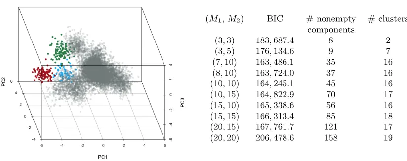
To fit HMM-VB given the dependence structure among the 8 variables, we only need to specify M1 andM2, the numbers of mixture components for the two variable blocks. If casted as a GMM, the HMM-VB has M1×M2 components for the full dimensional data. Model selection by BIC is conducted to select the optimal M1 and M2. Summaries on various model specifications are listed in Figure 5.1.1 (Right). The model withM1= 7 and

M2 = 10 has the lowest BIC and is thus chosen.

Recall that we search modes by MBW starting from the mean of every component that has been chosen by a data vector according to the maximum a posteriori rule. We call the components that have not been chosen by any data point the empty mixture components, while the others are nonempty. Figure 5.1.1 (Right) shows that even though the total number of nonempty mixture components increases with M1 andM2, the number of clusters after modal clustering remains relatively stable.

(M1,M2) BIC # nonempty # clusters components

(3,3) 183,687.4 8 2

(3,5) 176,134.6 9 7

(7,10) 163,486.1 35 16

(8,10) 163,724.0 37 16

(10,10) 164,245.1 45 16

(10,15) 164,822.9 70 17

(15,10) 165,338.6 56 16

(15,15) 166,313.4 85 18

(20,15) 167,761.7 121 17

(20,20) 206,478.6 158 19

Figure 2: (Left): Visualization of the simulated data in Section 5.1.1 based on the first three principal components (PC). The smallest three clusters are plotted in blue (54 observations), green (98), red (100), and the rest are in grey. (Right): Comparisons of BIC, total number of nonempty components and clusters under various model specifications (M1 and M2).

methods in Table 1 take less than one minute. For K-means, hierarchical clustering, and Mclust, we used the three R functionskmeans(with 20 starting points),hclustandMclust. In this analysis, we treat the 16 clusters found by MBW applied to the true mixture density as the ground truth. Hence, for K-means and hierarchical clustering, we manually set 16 as the number of clusters. The number of normal mixture components and the covariance structure are determined by BIC in theMclustpackage (the package version is 5.2.3). More specifically, we let Mclustsearch a maximum of 20 mixture components and then used the BIC to choose among all the default covariance matrix models, as computational errors were generated when searching over all the models. For this data set, the optimal number of clusters chosen by Mclust is 15. The modal GMM analysis is performed using the same C codes for fitting the HMM-VB model. We simply specified a single variable block containing all the 8 variables. The HMM-VB model is then reduced to a usual GMM. In addition, we let the total number of mixture components be 7×10 = 70.

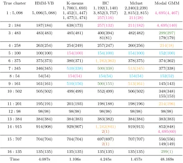
cluster and any E_i∗ is too small, the cluster is not listed in the ith row. Reversely, a cluster generated by a certain method may also cover a substantial portion of points from multiple true clusters. For instance, hierarchical clustering yields one small cluster of size 257, which contains both part of E₁∗ and E₂∗. A cluster of size 154 generated by K-means contains

E₅∗ andE₈∗. Therefore, a single cluster generated by a certain method may be reported in multiple rows. To indicate clearly such a case, the same color (except for black) is used to mark out a single cluster in any column. If a cluster is reported only once in any column, the result is shown in black (in other words, black is not a color code).

True cluster HMM-VB K-means HC Mclust Modal GMM 1,700(1,693) 1,192(1,140) 2,240(2,239)

1 : 5,098 5,096(5,088) 1,452(1,447) 3,852(3,757) 2,815(2,815) 4,695(4,467) 1,477(1,474) 257(116) 211(28)

2 : 184 187(184) 638(173) 257(132) 211(182) 4,695(140) 3 : 483 483(483) 485(481) 400(394) 482(482) 299(297)

81(81) 179(179)

4 : 258 263(254) 254(249) 257(247) 260(256) 214(18)

5 : 100 100(100) 154(100) 154(100) 154(100) 152(100)

6 : 375 375(373) 380(371) 1,242(362) 378(375) 374(362) 7 : 345 346(345) 510(338) 500(338) 513(345) 377(338) 8 : 54 54(54) 154(54) 154(54) 154(54) 152(52)

9 : 161 161(161) 510(156) 500(155) 513(161) 145(143) 10 : 502 505(502) 499(499) 552(499) 506(502) 348(348) 155(153) 11 : 201 195(191) 201(193) 198(188) 198(196) 214(196)

12 : 98 98(98) 98(98) 98(98) 98(98) 98(98)

13 : 384 384(384) 384(383) 383(382) 384(384) 383(383) 14 : 915 914(908) 929(907) 1,242(841) 919(913) 852(848)

2(1) 4,695(60)

15 : 707 704(704) 704(704) 697(697) 707(707) 556(556)

2(1) 149(149)

16 : 135 135(135) 135(135) 135(135) 135(135) 299(1)

Time 4.087s 1.106s 4.245s 1.457s 48.169s

Table 1: Comparisons of clustering performance among HMM-VB, K-means, hierarchical clustering (HC), Mclust, and modal GMM for the simulation data in Section 5.1.1.

Table 1 demonstrates that HMM-VB outperforms clearly the other methods in terms of matching the true clusters, especially for the rare clusters. K-means, hierarchical clustering, and Mclust tend to yield similar-sized clusters. All of them split the largest true cluster E₁∗

into 3 smaller ones. Except for HMM-VB, all the other four methods fail to correctly identify all three smallest clusters, E₅∗, E₈∗ and E₁₂∗ . Specifically, according to the four methods,

the number of clusters, K-means is faster than hierarchical clustering. Mclust is performed on 15 mixture components, while both HMM-VB and modal GMM are fitted using 70 mixture components. The fact that HMM-VB is much faster than modal GMM shows the computational advantage to regularize a general GMM by a variable block structure.

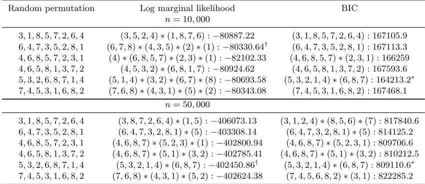
In addition, we use this simulation data to test the search algorithm for the variable block structure, which is described in Section 3.4. We run the algorithm with 6 different initial random permutations. The algorithm successfully selects the correct variable blocks according to the true distribution. Furthermore, to empirically demonstrate the efficiency of BIC for model selection, we also incorporate the comparison with (log) marginal likelihood approach in Table 2. Both approaches select the same model under the larger sample size.

Random permutation Log marginal likelihood BIC

n= 10,000

3,1,8,5,7,2,6,4 (3,5,2,4)∗(1,8,7,6) :−80887.22 (3,1,8,5,7,2,6,4) : 167105.9 6,4,7,3,5,2,8,1 (6,7,8)∗(4,3,5)∗(2)∗(1) :−80330.64† (6,4,7,3,5,2,8,1) : 167113.3 4,6,8,5,7,2,3,1 (4)∗(6,8,5,7)∗(2,3)∗(1) :−82102.33 (4,6,8,5,7)∗(2,3,1) : 166259 4,6,5,8,1,3,7,2 (4,5,3,2)∗(6,8,1,7) :−80924.62 (4,6,5,8,1,3,7,2) : 167593.6 5,3,2,6,8,7,1,4 (5,1,4)∗(3,2)∗(6,7)∗(8) :−80693.58 (5,3,2,1,4)∗(6,8,7) : 164213.2∗ 7,4,5,3,1,6,8,2 (7,6,8)∗(4,3,1)∗(5)∗(2) :−80343.08 (7,4,5,3,1,6,8,2) : 167468.1

n= 50,000

3,1,8,5,7,2,6,4 (3,8,7,2,6,4)∗(1,5) :−406073.13 (3,1,2,4)∗(8,5,6)∗(7) : 817840.6 6,4,7,3,5,2,8,1 (6,4,7,3,2,8,1)∗(5) :−403308.14 (6,4,7,3,2,8,1)∗(5) : 814125.2 4,6,8,5,7,2,3,1 (4,6,8,7)∗(5,2,3)∗(1) :−402800.94 (4,6,8,7)∗(5,2,3,1) : 809706.6 4,6,5,8,1,3,7,2 (4,6,8,7)∗(5,1)∗(3,2) :−402785.41 (4,6,8,7)∗(5,1)∗(3,2) : 810212.5 5,3,2,6,8,7,1,4 (5,3,2,1,4)∗(6,8,7) :−402450.86† (5,3,2,1,4)∗(6,8,7) : 809110.6∗ 7,4,5,3,1,6,8,2 (7,6,8)∗(4,3,1)∗(5,2) :−402624.38 (7,4,5,6,8,2)∗(3,1) : 822285.2

Table 2: Comparison of BIC and log marginal likelihood for model selection using 6 initial random permutations under two different sample sizes. We mark the model selected by BIC with ? and the model selected by log marginal likelihood with †. We use parentheses to indicate a particular variable block, and ∗to separate the different variable blocks.

5.1.2 No Information on Variable Blocks

Figure 3: Pairwise scatter plots of simulated data from Section 5.1.2. Colors indicate the cluster membership.

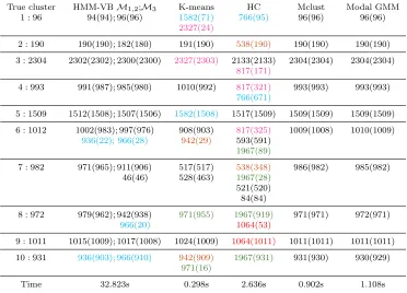
True cluster HMM-VBM1,2;M3 K-means HC Mclust Modal GMM

1 : 96 94(94); 96(96) 1582(71) 766(95) 96(96) 96(96) 2327(24)

2 : 190 190(190); 182(180) 191(190) 538(190) 190(190) 190(190) 3 : 2304 2302(2302); 2300(2300) 2327(2303) 2133(2133) 2304(2304) 2304(2304)

817(171)

4 : 993 991(987); 985(980) 1010(992) 817(321) 993(993) 993(993)

766(671)

5 : 1509 1512(1508); 1507(1506) 1582(1508) 1517(1509) 1509(1509) 1509(1509) 6 : 1012 1002(983); 997(976) 908(903) 817(325) 1009(1008) 1010(1009)

936(22); 966(28) 942(29) 593(591)

1967(89)

7 : 982 971(965); 911(906) 517(517) 538(348) 986(982) 985(982)

971(965);46(46) 528(463) 1967(28)

521(520) 84(84)

8 : 972 979(962); 942(938) 971(955) 1967(919) 971(971) 972(971)

979(962);966(20) 1064(53)

9 : 1011 1015(1009); 1017(1008) 1024(1009) 1064(1011) 1011(1011) 1011(1011) 10 : 931 936(903); 966(910) 942(909) 1967(931) 931(930) 930(929)

971(16)

Time 32.823s 0.298s 2.636s 0.902s 1.108s

Table 3: Comparison of clustering performance among three HMM-VB models, K-means, hierarchical clustering (HC), Mclust, and modal GMM for simulation data in Section 5.1.2. The first two HMM-VB models give the same results for major clusters.

variables. The number of components for each block chosen by BIC isMt= 7, t= 1, ...,5.

Model M2 is defined similarly as M1, but we reverse the ordering of the variables such thatx= (x5, x4, ..., x1). Lastly, we let M3 be a HMM-VB with 5 variable blocks ordered by a random permutation x= (x1, x3, x4, x2, x5). Table 3 shows the clustering results for the three HMM-VB models and the other four baseline methods. The format of the results in this table is the same as that for Table 1 in the previous section. Again we pre-set the number of clusters for K-means, hierarchical clustering, and modal GMM as the true value. The model specification for Mclust is similar to the previous experiment, but we allow Mclustto search for up to 12 Gaussian components. For clarity of presentation, clusters that share fewer than 5 points with any true cluster are not reported in Table 3. As expected

M1 andM2 yield very similar results. As discussed at the end of Section 4.1, when the ordering of the variable blocks is reversed, the GMM casted from the HMM-VB is essentially the same. Small differences may arise due to some random factors caused by initialization. We simply report results from one of the two models. Table 3 suggests that HMM-VB is quite robust to the ordering of the variables. Both K-means and hierarchical clustering fail to extract the cluster structures. As expected, both Mclust and modal GMM can accurately recover all the clusters because the data is generated according to the generic GMM model. The search scheme for selecting the optimal variable block structure determines that only one variable block is needed (that is, the usual GMM). This is consistent with the true model. However, Table 3 shows that although the HMM-VB with five blocks is not the right model, it can still perform reasonably well for clustering. This finding suggests that HMM-VB can be a new strategy to regularize a GMM, the complexity of which is normally only controlled by the number of components or constraints on the covariance matrices.

5.1.3 Large Data Size

Since HMM-VB is motivated by single-cell data analysis, where the sample size can be up to several millions, we now study the performance of HMM-VB for large data sets with moderately high dimensions. We let dimension d = 40, and sample size n ranges from 100,000, 1,000,000 and 5,000,000. The first 10 dimensions are generated from a 3-component GMM. The remaining 30 dimensions are generated from a 5-component GMM, where the mixture component proportions vary according to which normal component the first 10 dimensions are generated from. In addition, the covariance matrices of the last 30 dimensions are block diagonal, containing two blocks of sizes 10×10 and 20×20. Furthermore, by specifically designing the mean vectors and the transition probability matrix from the first 10 dimensions to the rest, the data generated contain 5 distinct normal components which correspond to 5 distinct clusters. The detailed description for the data generation is in Appendix E. The relative proportions for the 5 clusters are about 0.005, 0.045, 0.07, 0.18, and 0.7.

In this particular study, Mclust encounters some numerical errors when performing model selection. Because K-means and hierarchical clustering perform poorly in the previous two studies, we hereby focus on the comparison between VB and modal GMM. To fit HMM-VB, we divide the 40 dimensions into 3 blocks: x(1)_i = (xi,1, ..., xi,10),x(2)_i = (xi,11, ..., xi,20),

x(3)_i = (xi,21, ..., xi,40). According to the model specification, we let M1 = 3, M2 = 5, and

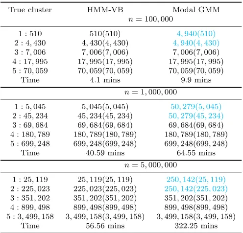
True cluster HMM-VB Modal GMM

n= 100,000

1 : 510 510(510) 4,940(510)

2 : 4,430 4,430(4,430) 4,940(4,430)

3 : 7,006 7,006(7,006) 7,006(7,006) 4 : 17,995 17,995(17,995) 17,995(17,995) 5 : 70,059 70,059(70,059) 70,059(70,059)

Time 4.1 mins 9.9 mins

n= 1,000,000

1 : 5,045 5,045(5,045) 50,279(5,045)

2 : 45,234 45,234(45,234) 50,279(45,234)

3 : 69,684 69,684(69,684) 69,684(69,684) 4 : 180,789 180,789(180,789) 180,789(180,789) 5 : 699,248 699,248(699,248) 699,248(699,248)

Time 40.59 mins 64.55 mins

n= 5,000,000

1 : 25,119 25,119(25,119) 250,142(25,119)

2 : 225,023 225,023(225,023) 250,142(225,023)

3 : 351,202 351,202(351,202) 351,202(351,202) 4 : 899,498 899,498(899,498) 899,498(899,498) 5 : 3,499,158 3,499,158(3,499,158) 3,499,158(3,499,158)

Time 56.56 mins 322.25 mins

Table 4: Comparison of clustering performance between HMM-VB and modal GMM for simulation study in Section 5.1.3.

Table 4 shows the clustering results for the two models for simulated data of three different sample sizes. HMM-VB correctly identifies all the clusters for the three data sets. However, modal GMM cannot separate the two smallest clusters. In addition, HMM-VB requires much shorter computation time than modal GMM, even though the equivalent GMM of the HMM-VB has 3×5×5 = 75 components. The difference in computation time is even more dramatic when the sample size is large. In order to detect more accurately the rare clusters by modal GMM, we could increase the number of mixture components. However, the increase may have to be large causing much slower computation.

5.1.4 Clustering Variation Study

To investigate the variation of clustering results for the above three simulations, we in addition randomly generate 100 replicates from the two variable blocks model in Section 5.1.1, 100 replicates from the 10-component GMMs with randomly generated covariance matrices described in Section 5.1.2, and only 10 replicates for the model in Section 5.1.3 due to the extensive computational time caused by large data size. We use the adjusted Rand index (ARI) (Rand, 1971) to assess the similarity between the clustering result by each method and the true cluster assignments. Summaries based on the ARI for the first two simulation studies are shown in Figure 4, and that for the last simulation is provided in Table 5.

Figure 4: Boxplots of ARI based on 100 replicates generated by simulations in Section 5.1.1 and 5.1.2.

by HMM-VB is not right, while Mclust and modal GMM are based on the correct model. Nevertheless, the boxed range of ARIs by HMM-VB overlaps with that by Mclust although the average by HMM-VB is lower. The best result is obtained by modal GMM. For the third simulation in Section 5.1.3, although both HMM-VB and modal GMM yield high ARIs, the average number of clusters obtained by HMM-VB is always the same or nearly the same as the true value, while that by modal GMM is consistently lower by one. Finally, we note that ARI measures overall similarity between clustering results. Thus small clusters matter less than large clusters for ARI. If finding rare clusters is important, we should not rely only on ARI to evaluate the methods. Results shown in Table 1, 3, and 4 can be more pertinent.

Sample size mean ARI median ARI sd ARI C¯ HMM-VB

100,000 1 1 0 5

1,000,000 1 1 0 5

5,000,000 0.9999 1 2.88×10−4 4.9 Modal GMM

100,000 0.9991 0.9991 5.74×10−5 4 1,000,000 0.9992 0.9991 2.88×10−4 4.1 5,000,000 0.9513 0.9991 0.15 4.1

5.2 Study of CyTOF Data

As a motivating example, current high-throughput flow cytometry experiments routinely measure 10∼20 parameters (cell markers/variables) on a large number of single cells. The current mass cytometry (CyTOF) can measure up to 50 parameters at a single cell level. A key first step to analyze this wealth of data is to partition the data (cells) from a blood or tissue sample into clusters based on the measured cell markers. The identified clusters are usually referred to as (cell) subsets.

Many studies adopt clustering based on mixture models to identify cell subsets objectively and automatically for single-cell data analysis (e.g., Boedigheimer and Ferbas (2008); Lo et al. (2008); Chan et al. (2008); Pyne et al. (2009); Aghaeepour et al. (2013); Lin et al. (2016)). One challenge encountered is that cell subsets of interest are typically of low frequencies (e.g., ∼0.01% of total cells), while it is important to detect cell heterogeneity, especially very low frequency cell subsets for subsequent analysis, e.g., to understand the association between cellular heterogeneity and disease progression (Darrah et al., 2007; Lin et al., 2015a; Seshadri et al., 2015; Corey et al., 2015).

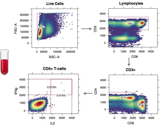
One important structure of the CyTOF data is a natural chain-like dependence among groups of variables (e.g., Roederer et al. (2004); Perfetto et al. (2004)). Biologists utilize such inherent property of the data to manually identify cell subsets by sequentially visualizing data on the groups of variables, known as manual gating, which has been extensively used in real data analysis. Specifically, the manual gating is a manual sequential process that visually demarcates cells in bounded regions (called gates) on histogram or 2-D scatter plot projections. Interestingly, the modal clustering technique has been applied to assist manual gating for cytometric data by Ray and Pyne (2012). Figure 5 provides a simplified illustration of the manual gating analysis on one flow cytometry data. Red lines are the gates, and cells within the region defined by the gates are identified as a specific cell subset. For example, to discriminate CD4+ T cells, which is one major cell subset, a sequence of subsetting procedures is performed. Two physical markers, Forward (FSC-A) and side (SSC-A) light scatter, are first used to distinguish lymphocytes from all the live cells.

Lymphocytes can then be further partitioned based on 3 fluorescence parameters: CD3, CD4, and CD8 cell-surface markers. CD4+ T cells are the subclass of lymphocytes having high values of CD3 and CD4 but low value of CD8. Within CD4+ T-cell populations, additional functional markers such as intracellular makers (IL2 and IFNg) can further distinguish many functionally different CD4+ T-cell subsets. The sequence of groups of markers to use is calledgating hierarchy, which is determined by expert knowledge. The shape and location of the gates are manually drawn. The gates are typically used to dichotomize the continuous marker expressions into binary value: positive and negative.

In manual gating analysis, the variables are grouped and ordered based on expert knowledge. By using the well-established gating hierarchy that projects cells on lower dimensions, each subplot provides a finer resolution of the cellular heterogeneity. In the sequential visualization process, any move one step further means a new group of variables are examined. Despite its wide usage, the manual gating analysis is highly subjective, time consuming, and hard to reproduce.

Figure 5: A simplified example of cell subsets identification by manual gating analysis. The flow cytometry measurements on single cells from a blood sample are shown using 4 heat maps of 2-D scatter plots projected on different dimensions (markers). The red lines on each subplots are called gates. Cells within the red lines are the subset of interest, which is subsetted and projected on the next subplot in the sequence. The percentages are the frequencies of the identified cell subsets relative to the total number of cells.

from mouse lung sample obtained from three C57BI6 wild-type mice and three Csf2rb−/− mice, which in total contains 46,204 single cells with 39 measured cell markers. According to the gating hierarchy provided in Becher et al. (2014), it defines roughly 11 variable blocks, with maximum block size 8 and minimum block size 1. Becher et al. (2014) performed automated clustering on a projected (latent) 2−dimensional space by first using nonlinear dimension reduction technique on the original 39−dimensional space. However, it has been studied, e.g. Lin et al. (2015b), that dimension reduction generates a “cluttered” display, which can prevent density estimation from accurately representing low probability regions. We first standardized the data to compensate for the nearly singular covariance matrix when a single Gaussian is fit despite the moderate dimension. This factor prevents the direct use of GMM. We note that HMM-VB encounters no difficulty in fitting the original data because of the smaller dimensions of the individual variable blocks. In order to compare modal GMM and HMM-VB, we work on the standardized data through the rest of the section.

We first fit the data using HMM-VB. There are 11 variable blocks. For the ith variable blocks with dimension lower than 4, we set the corresponding number of mixture components

Mi = 5. For thejth variable blocks with dimension between 5 and 7, we set the number of

CPU time per model fitting is 11.4 min. We then fit the data using GMM withM = 500. On the same iMac, the model fitting takes 284.2 min, 25 times longer than does HMM-VB. Modal clustering results in 232 clusters of size greater than 5.

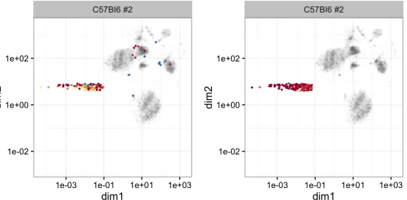
We compare the performance of the two models for clustering a relatively low probability region, which is shown in Figure 6. Specifically, Figure 6 compares the finer cellular compositions of one well separated region, which is visualized on two latent dimensions obtained from a dimension reduction technique applied to the original 39 dimensions, as provided by the result of Becher et al. (2014). HMM-VB (right subplot) uses 18 clusters to define this particular region. GMM (left subplot) uses 40 clusters to define the same region. However, some of the clusters include cells that are visually far away from the particular region. This result indicates that GMM has difficulty in estimating the structure of this moderately high-dimensional data.

Figure 6: Left: GMM clustering analysis for a particular data region of one selected mouse. Right: The corresponding HMM-VB clustering analysis. The data is shown in grey. Clustering results are in different colors with one color defines one cluster.

5.3 Examples of Very High Dimensional Data

We apply HMM-VB to two data sets with dimensiondn.

5.3.1 Single-Cell Genomics Data