R E S E A R C H A R T I C L E
Open Access
Outlier classification performance of risk
adjustment methods when profiling multiple
providers
Timo B. Brakenhoff
*, Kit C. B. Roes, Karel G. M. Moons and Rolf H. H. Groenwold
Abstract
Background: When profiling multiple health care providers, adjustment for case-mix is essential to accurately classify the quality of providers. Unfortunately, misclassification of provider performance is not uncommon and can have grave implications. Propensity score (PS) methods have been proposed as viable alternatives to conventional multivariable regression. The objective was to assess the outlier classification performance of risk adjustment methods when profiling multiple providers.
Methods: In a simulation study based on empirical data, the classification performance of logistic regression (fixed and random effects), PS adjustment, and three PS weighting methods was evaluated when varying parameters such as the number of providers, the average incidence of the outcome, and the percentage of outliers. Traditional classification accuracy measures were considered, including sensitivity and specificity.
Results: Fixed effects logistic regression consistently had the highest sensitivity and negative predictive value, yet a low specificity and positive predictive value. Of the random effects methods, PS adjustment and random effects logistic regression performed equally well or better than all the remaining PS methods for all classification accuracy measures across the studied scenarios.
Conclusions: Of the evaluated PS methods, only PS adjustment can be considered a viable alternative to random effects logistic regression when profiling multiple providers in different scenarios.
Keywords: Propensity score, Risk adjustment, Classification, Profiling, Random effects, Logistic regression, Simulation study
Background
In the last decades, performance of health care providers, for instance hospitals, has come under immense scrutiny. Government institutions, patients and providers them-selves are increasingly demanding performance indicators of the quality of care. These can be based on clinical out-come measures such as mortality or complication rates [1–3]. For example, when profiling (i.e., assessing the performance of ) well-established, high-risk procedures such as coronary artery bypass grafting (CABG), mortal-ity is considered an appropriate outcome measure and thus often used [2–4]. After adjustment for differences
*Correspondence:[email protected]
Julius Center for Health Sciences and Primary Care, University Medical Center Utrecht, PO Box 85500, 3508 GA, Utrecht, the Netherlands
in patient characteristics between providers, these mor-tality rates can be used to classify providers as perform-ing as expected (normal) or either better or worse than expected (outlying). Unfortunately, when using customary methodologies to adjust these outcome measures across providers, misclassification of provider performance is not uncommon, which may in turn have immense eco-nomic and societal implications [5–8].
When making comparisons between health care providers, an essential step is the adjustment for dif-ferences between providers in the risk profiles of their patients. This is often referred to as risk adjustment. Taking into account the differences in relevant patient characteristics between providers (also known as case-mix) is crucial to obtain accurate and reliable estimates of provider performance [1,9]. However, many studies have
found that traditional regression based methods lead to inadequate adjustment for case-mix and are thus unable to correctly classify providers in a consistent manner. In addition, this classification performance is highly depen-dent on the statistical model applied and the classification criteria used [1,3,6,10–13], especially when low-volume providers are included or outcomes are rare [14–17].
Propensity score (PS) methods have previously been put forward for risk adjustment [18]. These methods showed superior performance over conventional multi-variable regression in several observational dichotomous treatment settings, e.g. when samples are small [19–27]. Furthermore, a simulation study [28] found that some PS methods performed on par with multivariable regression when profiling several providers, in line with results found in analogous settings where multiple treatment options were compared [29–32]. Seeing as PS methods have cer-tain attractive advantages over conventional regression including the easy assessment of balance on relevant case-mix variables between multiple providers and their flexi-bility for different types of outcomes [20,22], PS methods are considered viable alternatives for risk adjustment prior to provider profiling.
However, extended methodological research on the per-formance of PS and regression based methods when profiling many providers are still lacking [33]. The aim of this study was to compare several PS methods with conventionally used (hierarchical) logistic regres-sion on their ability to identify (or classify) health care providers that performed better or worse than expected (i.e. outliers). A simulation study, based on empirical data from the field of cardiac surgery, was used to assess how the classification accuracy of each method dif-fered in varying circumstances that may be encountered in practice.
Methods
Risk adjustment methods
Before detailing the set up of the simulation study, the following risk adjustment methods are explained: fixed effects logistic regression (LRF), random effects logistic
regression (LRR), generalized propensity score (gPS)
case-mix adjustment (gPSA), gPS inverse probability weighting
(gPSW), gPS inverse probability weighting with trimming
(gPSWT) and gPS marginal mean weighting through
strat-ification (gPSMWS).
Fixed and random effects logistic regression
When dealing with dichotomous outcomes, such as mortality, multivariable logistic regression models are traditionally used for risk adjustment. These models can include the individual providers of which we want to determine the performance as either fixed or random effects. Fixed effects logistic regression (LRF) assumes
that all variation between providers is due to differences in case-mix and that the model specification is correct. By including providers as dummy variables, direct com-parisons between providers can be made [34, 35]. Ran-dom effects logistic regression (LRR) accounts for the
increased similarity between patients attending the same provider, the hierarchical structure of the data, and allows for residual variance between providers that may not be attributable to performance. In addition, the dimension-ality of the model is greatly reduced by only estimating the parameters of the distribution underlying the provider effects [36]. LRR is considered especially suitable when
between-provider variation is to be quantified, provider-level variables are measured, or low volume providers are to be profiled [6,13,34,37,38].
How the provider effects are included in the model can have profound consequences on the accuracy of classi-fying providers as either normal or outliers. As provider effects are assumed to come from an underlying distri-bution in LRR, effect estimates of providers (especially
those with low volume) can borrow information from the other providers, shrinking these effects towards the mean of all providers [34]. This results in the identification of fewer performance outliers as compared to whenLRF is
used [35–40]. Given the fundamental difference in how the model is formulated, the decision whether to useLRF
or LRR is largely dependent on the goal of the profiling
exercise. At present, most papers advocate the use ofLRR
due to the hierarchical nature of provider profiling, and its conservativeness in identifying outliers.
Generalized propensity score methods
mortality and thus do not qualify as a confounder. For multiple provider comparisons, the generalized propen-sity score (gPS) can be used to adjust for observed case-mix variables. The gPS is described by Imbens [29] as the conditional probability of attending a particular provider given case-mix variables, and was further devel-oped by Imai & van Dyk [41]. The gPSs of each patient for each provider can be estimated using multinomial logis-tic regression including all relevant observed case-mix variables.
There are several different ways to utilize the extracted gPSs to determine the average performance of each provider. In gPS case-mix adjustment (gPSA), provider
effects on the outcome are conditional on the gPSs (for further details see: [31, 42]). For gPS weighting (gPSW)
the sample is first re-weighted by the inverse gPS of the provider actually attended. In the weighted sample, marginal provider effects can be estimated by only includ-ing the providers in the outcome model (for further details see: [31]). Extreme weights can be trimmed to a certain percentile to reduce the influence of outlying weights and potential model misspecification (as applied in gPSWT).
However, this can also lead to biased estimates due to infe-rior risk adjustment [43].gPSMWScombines elements of
gPS stratification and gPSW and has been suggested to
be superior togPSW in both a binary and multiple
treat-ment setting [32, 44, 45]. In this method, the gPSs for each provider are first stratified into several categories prior to weighting each individual by his/her representa-tion within their stratum. Subsequently, marginal provider effects can be estimated just as in gPSW (see [44] for
a detailed description). While other methods have also been described in the literature, such as gPS stratifica-tion [46] or gPS matching [30, 46, 47], these methods have either been shown to perform worse than the afore-mentioned methods [22, 27, 48, 49] or are logistically impractical when dealing with large numbers of providers [30,44,47].
Simulation study
A Monte Carlo simulation study was conducted based on empirical data from the field of cardiac surgery. This allowed us to mimic a situation with perfect risk adjust-ment in which the observed outlier classification accuracy of each method was compared with true outlier status as fixed in each generated dataset. Several parameters were varied across different scenarios each simulated 1000 times (see sectionScenarios). Simulations were peformed using R (v3.1.2) [50]. R scripts used for the simulation study are available upon request.
Data source
Open heart surgery is a field that has been subject to many developments in risk-adjusted mortality models
for quality control in the last decades [4, 40]. A selec-tion of anonymized data from the Adult Cardiac Surgery Database provided by the Netherlands Association of Cardio-Thoracic Surgery was used as a realistic founda-tion for the simulafounda-tion study.
The Adult Cardiac Surgery Database contains patient-and intervention characteristics of all cardiac surgery per-formed in 16 centers in the Netherlands as of 1 January, 2007. This dataset has previously been described and used by Siregar et al. for benchmarking [51,52]. For the sim-ulation study described in this paper, all patients from the 16 anonymized centers undergoing isolated CABG with an intervention date between 1 January, 2007 and 31 December, 2009 were included in the cohort. The average in-hospital mortality was 1.4%, ranging from 0.7 to 2.3%. The center indicator variable and outcome measure (in-hospital mortality) were removed from the dataset. Of the dichotomous variables included in the EuroSCORE, only those with an overall incidence over 5% were used. The final dataset was thus comprised of the following eight relevant predictors of mortality following CABG: age (centered), sex, chronic pulmonary disease, extracardiac arteriopathy, unstable angina, LV dysfunction moderate, recent myocardial infarction, and emergency interven-tion. This final dataset represented the case-mix pro-file of 25114 patients included in the selected cohort and was used to generate the data for the simulation study.
Data generation
Using a bootstrap procedure, patients were resampled from the final dataset selected from the empirical data described above. As such, samples were constructed of a desired size containing patients with realistic case-mix profiles. For each bootstrap sample, the eight case-mix variables (Z1,. . .,Z8) were included as covariates in a multinomial logistic regression model to determine each patients probability of assignment to each provider:
πk =
eαk+βk1Z1+...+βk8Z8 K
j
eαj+βj1Z1+...+βj8Z8
, (1)
where k represents a provider with k = {1,. . .,K}, αk
is the provider-specific intercept andβk1,. . .,βk8are the provider-specific coefficients for each case-mix variable. These coefficients were set equal within each provider (βk1 = . . . = βk8), yet differed between providers, with coefficient values drawn from a uniform distribution between 0 and 1. The coefficients of one provider, which acted as reference, were all set to 0.
of patients per provider as determined in each scenario, patients were continually resampled until each provider (k) had its required volume (nk) of patients. The amount
of patients in the final sample (N) was dependent on the number of providers (K) and the volumes of the providers (nk), which varied over the scenarios described in section
Scenarios.
Each patient’s value on the dichotomous outcome vari-able (Y) was generated using a random intercept logistic regression model:
logit[pik]=γ00+α0k+β1Z1ik+...+β8Z8ik, (2)
wherepik is the probability of mortality of theith patient
attending the kth provider, γ00 is the overall intercept, α0k are the provider-specific random intercepts, and
Z1ik,. . .,Z8ik correspond to each patient’s scores on the
case-mix variables. α0k ∼ N
μ,σ2, whereμ = 0 for
normal providers and μ = ±H ∗ σ for performance
outliers that are either below or above average. H thus represents the amount of standard deviations by which the normal distribution is shifted when drawing the ran-dom intercepts of thetrueoutlying providers.σ was set equal to 0.1942, corresponding to the standard deviation of the provider-specific intercepts found when fitting a random intercepts model on the full cohort of the dataset described in section Data source. When H = 2 the mean of the random effects distributions of the outlying providers are then 0.3884 and -0.3884, corresponding to odds ratios of 1.475 and 0.678 respectively, keeping all else constant. Note that the overlap between the normal and outlier distributions is actually larger in practice, due to sampling variability. In a simple case, assuming an average incidence of the outcome of 10%, this distance is reduced to about 1.75∗σ.
The coefficients of the case-mix variablesβ1,. . .,β8 corresponded to the odds ratios of the original EuroSCORE prediction model [53]. The average inci-dence of the outcome over all providers was fixed by manipulating the overall intercept (γ00) of the outcome model. In addition, each provider was required to have an incidence of the outcome of at least 1% to prevent separation and estimation problems when using the risk adjustment methods.
In this data generating mechanism, the case-mix vari-ables acted as confounders of the provider-outcome relation. As no interaction terms were included in the model, the provider effects were assumed constant over the different levels of the case-mix variables. Given the use of a random intercepts model to generate the out-come,LRRand the gPS methods were favored overLRF.
Also note that both the gPS (Eq. 1) and outcome mod-els (Eq. 2) were perfectly specified and contained the
same relevant case-mix variables. While a strong assump-tion, this reduced the variability in performance over simulations and limited the complexity of the simula-tion study. As such, LRR and gPSA were expected to
have comparable performance due to the similarity of the methods. Investigations into the consequences of model misspecification were outside the scope of the current study.
Scenarios
The parameters deemed relevant to manipulate are out-lined below. Table1contains the parameter settings of the studied scenarios.
• The number of providers,K : 10, 20, 30, 40, or 50.
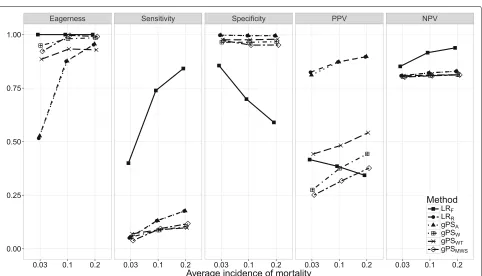
• The average incidence of mortality,p··: 3, 10 or 20%.
• The percentage of true outliers,P(out): 8, 20 or 40%. This ensured an equal number of true outliers selected from both outlier distribution for eachK studied.
• The amount of standard deviations the outlier random intercept distribution was shifted,H : 1, 2, 3, or 4.
• Outliers were either drawn from both outlier distributions (S=2) or only from the below-average performance distribution (S=1).
• Half of the providers were allocated either
min(nk)=500ormin(nk)=1000patients, while
the other half were always of sizemax(nk)=1000.
• Whenmin(nk)=500, on average either half,
P(nmin)=0.5, or all,P(nmin)=1, of outlying providers had a sample size of 500. This allowed us to investigate the consequences of a potential correlation between provider volume and quality [17,54,55].
Statistical analysis
The risk adjustment methods introduced earlier, were applied on each of the generated datasets. InLRFa logistic
Table 1Parameter Settings of Scenarios Studied Through Simulations
Scenario K p·· P(out) H S min(nk) P(nmin)
1 10-50 0.10 0.2 2 2 1000 0.5
2 50 0.03-0.20 0.2 2 2 1000 0.5
3 50 0.10 0.08-0.4 2 2 1000 0.5
4 50 0.10 0.2 1-4 2 1000 0.5
5 50 0.10 0.2 2 1-2 1000 0.5
6 50 0.10 0.2 2 2 500-1000 0.5
7 50 0.10 0.2 2 2 500 0.5-1
regression model only including the case-mix variables (Z1,. . .,Z8) was first fit to extract the overall intercept. Next, a second logistic regression model was fit without intercept including allK providers as dummy variables as well as Z1,. . .,Z8. Provider effects were classified as below or above average outliers if their 95% Wald confidence intervals did not include the overall inter-cept extracted from the first logistic regression model. In LRR a random intercepts logistic regression model
was fit including theK providers as random effects and Z1,. . .,Z8 as fixed effects. Providers of which the empiri-cal Bayes effect estimate deviated more than two observed standard deviations from the overall intercept of the fitted model were classified as outliers.
For the four gPS methods applied to the generated data sets, outliers were classified in identical fashion as described forLRR. ForgPSAa random intercepts logistic
regression model was fit including theKproviders as ran-dom effects andK−1 gPSs as fixed effects. IngPSW, each
patient was assigned a weight equal to the inverse of the gPS of the provider actually attended. A weighted random intercepts logistic regression was then performed as in LRRwith only theKproviders included as random effects.
gPSWT was identical togPSW, except that the highest 2%
of weights were trimmed to the 98th percentile based on results from similar scenarios in [43]. The determina-tion of the optimal trimming threshold was beyond the scope of this study. ForgPSMWSthe gPSs for each provider
were first stratified intoL = 5 strata, determined suffi-cient to remove over 90% of the selection bias [25,56,57]. Next the marginal mean weight (MMW) was calculated for each patient according to the formula described by Hong [44]:
MMW = nsk∗Pr(X=k)
nX=k,sk , (3)
where nsk is the number of patients in stratum s of provider k, Pr(X = k) is the proportion of patients assigned to providerkin the observed dataset andnX=k,sk is the amount of patients in stratum sk that actually
attended provider k. The MMWs were then used to
weight the sample as in gPSW with the following
anal-ysis and outlier classification proceeding in an identical manner.
The logistic regression models in LRF were fit using
the function glm from the stats package, part of the R program [50]. The random intercept logistic regression models applied in all other methods (LRR, gPSA, gPSW,
gPSWT,gPSMWS) were fit using the functionglmer from
the lme4package [58]. All models used in each method were properly specified, had the correct functional form and did not include interactions.
Classification performance
The classification accuracy of each risk adjustment method was evaluated by comparing theobserved classifi-cation of each provider as normal or outlying with thetrue status, as determined when generating the data. While alternative methods are available to classify outliers, the approach presented above suffices to enable a fair compar-ison of the different risk adjustment methods. Traditional classification accuracy performance measures including sensitivity, specificity, positive predictive value (PPV), and negative predictive value (NPV) were computed for each generated data set and averaged over all simulations. In addition, 90th percentile confidence intervals were cal-culated for each of these performance measures. Finally, a measure of classification eagerness was considered by calculating the proportion of simulated datasets in which at least one outlier (not necessarily a true outlier) was observed.
Results
Figures1,2,3,4,5,6and7show the classification perfor-mance of different risk adjustment methods for all studied scenarios (see Table 1). The 90th percentile confidence intervals over all bootstrap samples of these performance measures are displayed in Tables 2, 3, 4, 5, 6, 7 and 8 in the Appendix. Across all scenarios, the eagerness of LRF surpassed that of the gPS methods and LRR. As
these latter methods used random effects models to adjust for case-mix, conservativeness was to be expected. Of the gPS methods, gPSW and gPSMWS were most eager
to identify outliers, while gPSA was most conservative
with a performance identical to LRR. LRF consistently
had a much higher sensitivity (∼ 75%) than the other methods (∼ 15%), of which LRR and gPSA scored
sev-eral percentage points higher than their counterparts. gPS methods and LRR had very high specificities (between
90 and 100%) across the board with LRF coming in at
75%. As for the PPV,LRRandgPSAsystematically scored
best around 90%, withLRF,gPSW andgPSMWS
perform-ing worst with PPVs around 30%. With respect to the NPV, all gPS methods andLRRhad almost identical
per-formance (∼ 80%). LRF consistently scored about 10%
higher.
Scenario 1: number of providers. Figure 1 shows the effect of K on classification performance. As expected, the eagerness of all methods quickly approach 100% for increasingK. Even though the sensitivity, specificity, and NPV of the gPS methods andLRRseemed largely
unaf-fected byK,LRRandgPSAhad a slightly higher sensitivity
compared to the other methods whenKapproached 50. While the PPV ofLRR,gPSA, andLRFdecreased by about
8%, the PPV ofgPSW andgPSWT increased by about 12
Fig. 1The eagerness, sensitivity, specificity, positive predictive value (PPV), and negative predictive value (NPV) for differing amounts of providers (K), when using different risk adjustment methods. All other parameters were fixed (see scenario 1 of Table1)
Fig. 3The eagerness, sensitivity, specificity, positive predictive value (PPV), and negative predictive value (NPV) for different proportions of true outliers (P(out)) when using different risk adjustment methods. All other parameters were fixed (see scenario 3 of Table1)
Fig. 5The eagerness, sensitivity, specificity, positive predictive value (PPV), and negative predictive value (NPV) for the amount of outlier distributions (S) when using different risk adjustment methods. All other parameters were fixed (see scenario 5 of Table1)
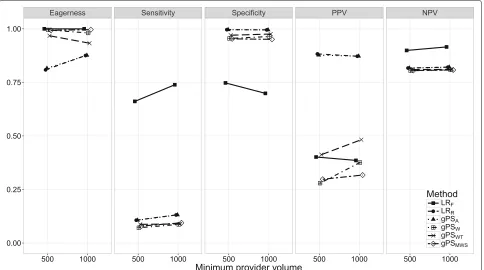
Fig. 7The eagerness, sensitivity, specificity, positive predictive value (PPV), and negative predictive value (NPV) for different percentages of outliers being allocated the minimum sample size,P(nmin), when using different risk adjustment methods. All other parameters were fixed (see scenario 7 of Table1)
sloped downwards, before leveling off from K = 30 onwards.
Scenario 2: incidence of mortality. In Fig.2the influence ofp·· on classification performance was investigated. All methods approached an eagerness of 100% asp··rose with LRRandgPSAincreasing the most. Whenp·· = 0.03, the
sensitivity of gPS methods andLRR did not surpass 10%
while that ofLRF dropped below 40%. Asp·· increased, this rose by about 12% for LRR, gPSA andgPSMWS, and
over 45% forLRF. Only the specificity ofLRF was
influ-enced byp··, dropping by about 25% asp·· increased. As for the PPV, all gPS methods andLRRhad a positive
rela-tionship with p··, while LRF decreased as p·· rose. The
NPV of all methods was mainly unaffected byp··; only LRFdropped towards the level of the other methods when
p··=0.03.
Scenario 3: percentage of true outliers. The influence of P(out)on classification performance is explored in Fig.3. IncreasingP(out)had little influence on the eagerness or specificity of all methods. Only the sensitivity ofLRRand
gPSA seemed to sharply decline towards the same level
as the other gPS methods (7%) asP(out) increased. The PPV of all methods had a strong positive relationship with P(out), withLRF,gPSW andgPSWT rising by about 25%,
andLRR andPSA rising by about 10%. The NPV of all
methods decreased asP(out)increased. Especially the gPS methods andLRRall decreased in identical fashion by over
20%. As both NPV and PPV are influenced by the preva-lence (in our case the proportion of true outliers) these results were to be expected.
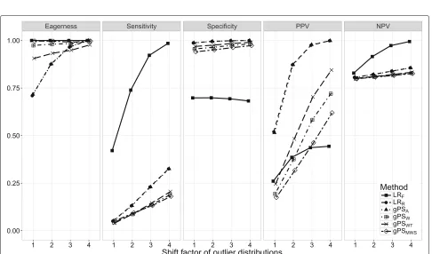
Scenario 4: outlier distribution shift. The relationship betweenHand classification performance was explored in Fig.4. As expected, the eagerness of all methods increased towards 100% asHreached 4. The sensitivity of all meth-ods was positively related toH, with LRF increasing by
more than 50% and LRR andgPSAby about 25%, about
10% more than the PS weighting methods. While the specificity remained unchanged, the PPV increased for all methods, withgPSWTincreasing most by about 50%. The
PPV ofLRFleveled off after an increase of about 20%. The
NPV ofLRFwas the only one affected, increasing by about
20% asHapproached 4.
Scenarios 5 through 7. The effect of S, min(nk),
and P(nmin) on classification performance is shown in Figs. 5, 6 and 7. As expected, with performance out-liers on both sides (S = 2) all performance measures increased at least slightly for all methods. Including both small and large providers (min(nk) = 500) had a small
effect on classification performance. ForLRFthe
PPV decreased incrementally. Of the remaining meth-ods, the PPV of gPSW andgPSWT and the eagerness of
gPSAandLRRdecreased slightly. When all outliers were
allocated the minimum sample size (P(nmin) = 1), the sensitivity, specificity and NPV ofLRRand the gPS
meth-ods was unchanged. For the PPV, LRRandgPSAslightly
declined while gPSW and gPSWT slightly increased.
All accuracy measures of LRF slightly decreased as
P(nmin)increased, with sensitivity dropping the most by about 10%.
Discussion
In this study, the outlier classification performance of gen-eralized propensity score (gPS) risk adjustment methods was compared to traditional regression-based methods when profiling multiple providers.Fixed effects logistic regression (LRF) consistently had the highest eagerness,
sensitivity and negative predictive value (NPV), yet had a low specificity and positive predictive value (PPV). Of the random effects methods, gPS adjustment (gPSA) and
random effects logistic regression (LRR) were the most
conservative, yet performed equally well or better than all the remaining gPS methods for all classification accu-racy measures across the studied scenarios. A decision on which of the studied methods to use should depend on the goal of the profiling exercise, taking into consideration the distinct differences between fixed and random effects risk adjustment methods outlined in section Fixed and random effects logistic regression.
While all gPS methods and LRRused a random
inter-cepts model in the analysis stage,LRFsolely included fixed
effects. This was evident in the large performance differ-ences between these methods and is in line with many published simulation studies examining fixed and ran-dom effects regression [6, 37, 39]. Also notable was the reactivity ofLRF to changes in most parameters as
com-pared to the more stable random effects methods, for example with the sensitivity dropping sharply when out-liers differed little from normal providers or the when the outcome was rare.
The sensitivity of all random effects methods was low across all scenarios. This was to be expected as the maximum achievable sensitivity was limited by the substantial overlap of the observed normal and outlier provider effect distributions. The degree of overlap was determined by the fixed standard deviation of the ran-dom effects distributions from which the effects were drawn, sampling variability and the distance between the normal and outlier distributions. When this dis-tance (H) was increased the sensitivity quickly rose (see Fig.4).
The overall identical performance ofgPSAandLRRwas
to be expected given the inclusion of the same case-mix variables in both the gPS and outcome models. However,
the inferior performance of the gPS weighting meth-ods across all studied scenarios was surprising. Earlier findings suggested that gPS weighting (gPSW)
outper-formed gPS weighting with trimming (gPSWT) and had a
performance on par with that of gPSA andLRR [28]. In
the current study, trimming outlying weights had a posi-tive effect on performance. Also unexpected was how gPS marginal mean weighting through stratification (gPSMWS)
performed even worse in the majority of scenarios, dis-puting earlier claims of its superior performance [32,44, 45]. A possible reason for this may be our omission of an essential step of the MMWS method, in which individuals that fall out of the common area of support are removed. This was done because for an increasing number of providers, effective sample sizes were reduced to 0. In addition, to ensure a fair and pragmatic comparison, the MMWS method was applied under similar circumstances as the other gPS methods where the assessment of balance across groups is often ignored because there is no consen-sus on how to do this properly when comparing multiple providers.
To explore the effect of many different parameters on classification performance, a simulation study was used. Due to the enormous amount of parameter combinations, a full factorial design was abandoned in favor of a uni-variate investigation of each parameter. Some parameter settings that might be seen in practice, such as provider volumes smaller than 500 patients, were omitted to pre-vent separation and convergence problems in addition to limiting the scope of the study. While scenarios were chosen to reflect realistic and sometimes extreme situa-tions that may be encountered when profiling providers, more extensive investigation into the effect of the studied parameters and others may be necessary to judge the con-sistency of the results in all possible settings. Furthermore, several choices made when generating the data (such as the parameters of the provider effect distributions) will not reflect situations encountered in practice. Even so, it is not likely that this would affect the presented results. Strengths of the approach utilized in this paper were that the covariance structure of the case-mix variables was extracted from an empirical dataset and that associ-ations between the case-mix variables and the outcome were taken from the original EuroSCORE model. Further-more, drawing provider-specific random intercepts from three normal distribution of which only the mean dif-fered was deemed theoretically realistic. This trimodal approach allowed the investigation of all cells of the con-fusion matrix and has been applied in similar simulation studies [6].
distributions prior to fitting the outcome model. How-ever, this step is often omitted in practice as there is no consensus on how to assess balance on multiple case-mix variables when considering more than three providers. Disregarding it in our simulation study allowed us to evaluate all methods including their drawbacks. Furthermore, all PS and outcome models were assumed properly specified with no unmeasured confounding by including all the case-mix variables used for data gener-ation in the analysis phase. While the authors acknowl-edge that performance of the risk adjustment methods may differ in more realistic situations, the results from this controlled simulation study may act as reference for essential further studies into the effect of misspec-ification and unobserved confounding on classmisspec-ification performance. Several authors have already recently com-mented on the potential effects of misspecification in comparable, yet simpler situations [59, 60]. Lastly, it is important to stress that the data was generated under the assumption of a random intercepts model, and thus inherently favored the random effects methods. Fur-ther simulation studies may be performed to investigate the effect of using different data generating mechanisms on the performance of the considered risk adjustment methods.
Conclusions
This study has demonstrated that of the gPS methods studied, only gPS case-mix adjustment can be considered as a viable alternative to random effects logistic regression when profiling multiple providers in different scenarios. The former method may be preferred as it allows the assessment of balance across providers prior to fitting the outcome model. Additionally, the many different scenar-ios investigated can give guidance on the classification performance that may be expected when dealing with different provider profiling exercises.
Appendix
Confidence interval tables
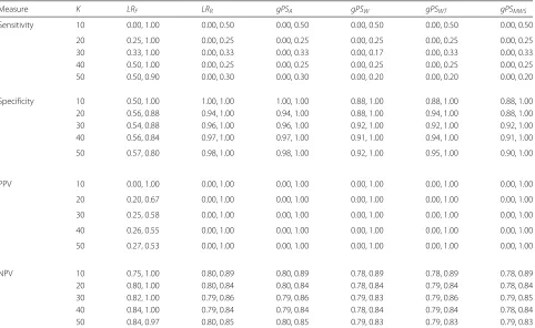
The following 7 tables show the 90th percentile confi-dence intervals of the performance measures assessed for each method within each scenario. Note that the number of true outliers in the studied scenarios depended on the amount of providers (K) and the percentage of true out-liers (P(out)). As a result performance measures such as the sensitivity could only take on a limited number of values within each sample. In addition, a difference of one in the number of outliers observed would also lead to a relatively large change in the studied performance measures.
Table 2The 90th percentile confidence intervals for all performance measure estimates of each method for Scenario 1 in Table1
(corresponding to Fig.1)
Measure K LRF LRR gPSA gPSW gPSWT gPSMWS
Sensitivity 10 0.00, 1.00 0.00, 0.50 0.00, 0.50 0.00, 0.50 0.00, 0.50 0.00, 0.50
20 0.25, 1.00 0.00, 0.25 0.00, 0.25 0.00, 0.25 0.00, 0.25 0.00, 0.25 30 0.33, 1.00 0.00, 0.33 0.00, 0.33 0.00, 0.17 0.00, 0.33 0.00, 0.33 40 0.50, 1.00 0.00, 0.25 0.00, 0.25 0.00, 0.25 0.00, 0.25 0.00, 0.25 50 0.50, 0.90 0.00, 0.30 0.00, 0.30 0.00, 0.20 0.00, 0.20 0.00, 0.20
Specificity 10 0.50, 1.00 1.00, 1.00 1.00, 1.00 0.88, 1.00 0.88, 1.00 0.88, 1.00 20 0.56, 0.88 0.94, 1.00 0.94, 1.00 0.88, 1.00 0.94, 1.00 0.88, 1.00 30 0.54, 0.88 0.96, 1.00 0.96, 1.00 0.92, 1.00 0.92, 1.00 0.92, 1.00 40 0.56, 0.84 0.97, 1.00 0.97, 1.00 0.91, 1.00 0.94, 1.00 0.91, 1.00
50 0.57, 0.80 0.98, 1.00 0.98, 1.00 0.92, 1.00 0.95, 1.00 0.90, 1.00
PPV 10 0.00, 1.00 0.00, 1.00 0.00, 1.00 0.00, 1.00 0.00, 1.00 0.00, 1.00
20 0.20, 0.67 0.00, 1.00 0.00, 1.00 0.00, 1.00 0.00, 1.00 0.00, 1.00
30 0.25, 0.58 0.00, 1.00 0.00, 1.00 0.00, 1.00 0.00, 1.00 0.00, 1.00
40 0.26, 0.55 0.00, 1.00 0.00, 1.00 0.00, 1.00 0.00, 1.00 0.00, 1.00
50 0.27, 0.53 0.00, 1.00 0.00, 1.00 0.00, 1.00 0.00, 1.00 0.00, 1.00
NPV 10 0.75, 1.00 0.80, 0.89 0.80, 0.89 0.78, 0.89 0.78, 0.89 0.78, 0.89
20 0.80, 1.00 0.80, 0.84 0.80, 0.84 0.78, 0.84 0.79, 0.84 0.78, 0.84 30 0.82, 1.00 0.79, 0.86 0.79, 0.86 0.79, 0.83 0.79, 0.86 0.79, 0.85 40 0.84, 1.00 0.79, 0.84 0.79, 0.84 0.78, 0.84 0.79, 0.84 0.78, 0.84 50 0.84, 0.97 0.80, 0.85 0.80, 0.85 0.79, 0.83 0.79, 0.83 0.79, 0.83
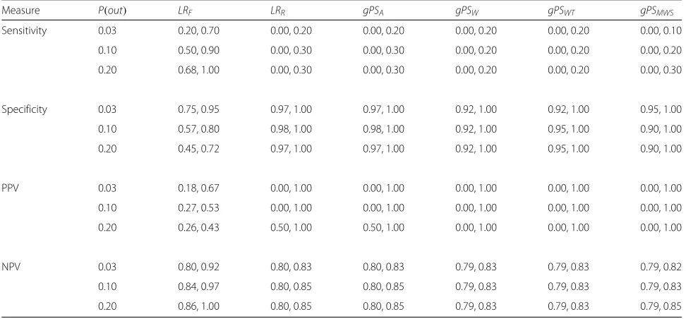
Table 3The 90th percentile confidence intervals for all performance measure estimates of each method for Scenario 2 in Table1
(corresponding to Fig.2)
Measure p.. LRF LRR gPSA gPSW gPSWT gPSMWS
Sensitivity 0.03 0.20, 0.70 0.00, 0.20 0.00, 0.20 0.00, 0.20 0.00, 0.20 0.00, 0.10
0.10 0.50, 0.90 0.00, 0.30 0.00, 0.30 0.00, 0.20 0.00, 0.20 0.00, 0.20
0.20 0.68, 1.00 0.00, 0.30 0.00, 0.30 0.00, 0.20 0.00, 0.20 0.00, 0.30
Specificity 0.03 0.75, 0.95 0.97, 1.00 0.97, 1.00 0.92, 1.00 0.92, 1.00 0.95, 1.00
0.10 0.57, 0.80 0.98, 1.00 0.98, 1.00 0.92, 1.00 0.95, 1.00 0.90, 1.00
0.20 0.45, 0.72 0.97, 1.00 0.97, 1.00 0.92, 1.00 0.95, 1.00 0.90, 1.00
PPV 0.03 0.18, 0.67 0.00, 1.00 0.00, 1.00 0.00, 1.00 0.00, 1.00 0.00, 1.00
0.10 0.27, 0.53 0.00, 1.00 0.00, 1.00 0.00, 1.00 0.00, 1.00 0.00, 1.00
0.20 0.26, 0.43 0.50, 1.00 0.50, 1.00 0.00, 1.00 0.00, 1.00 0.00, 1.00
NPV 0.03 0.80, 0.92 0.80, 0.83 0.80, 0.83 0.79, 0.83 0.79, 0.83 0.79, 0.82
0.10 0.84, 0.97 0.80, 0.85 0.80, 0.85 0.79, 0.83 0.79, 0.83 0.79, 0.83
0.20 0.86, 1.00 0.80, 0.85 0.80, 0.85 0.79, 0.83 0.79, 0.83 0.79, 0.85
p..= average mortality rate over providers; PPV = positive predictive value; NPV = negative predictive value
Table 4The 90th percentile confidence intervals for all performance measure estimates of each method for Scenario 3 in Table1
(corresponding to Fig.3)
Measure P(out) LRF LRR gPSA gPSW gPSWT gPSMWS
Sensitivity 0.03 0.20, 0.70 0.00, 0.20 0.00, 0.20 0.00, 0.20 0.00, 0.20 0.00, 0.10
0.10 0.50, 0.90 0.00, 0.30 0.00, 0.30 0.00, 0.20 0.00, 0.20 0.00, 0.20
0.20 0.68, 1.00 0.00, 0.30 0.00, 0.30 0.00, 0.20 0.00, 0.20 0.00, 0.30
Specificity 0.03 0.75, 0.95 0.97, 1.00 0.97, 1.00 0.92, 1.00 0.92, 1.00 0.95, 1.00
0.10 0.57, 0.80 0.98, 1.00 0.98, 1.00 0.92, 1.00 0.95, 1.00 0.90, 1.00
0.20 0.45, 0.72 0.97, 1.00 0.97, 1.00 0.92, 1.00 0.95, 1.00 0.90, 1.00
PPV 0.03 0.18, 0.67 0.00, 1.00 0.00, 1.00 0.00, 1.00 0.00, 1.00 0.00, 1.00
0.10 0.27, 0.53 0.00, 1.00 0.00, 1.00 0.00, 1.00 0.00, 1.00 0.00, 1.00
0.20 0.26, 0.43 0.50, 1.00 0.50, 1.00 0.00, 1.00 0.00, 1.00 0.00, 1.00
NPV 0.03 0.80, 0.92 0.80, 0.83 0.80, 0.83 0.79, 0.83 0.79, 0.83 0.79, 0.82
0.10 0.84, 0.97 0.80, 0.85 0.80, 0.85 0.79, 0.83 0.79, 0.83 0.79, 0.83
0.20 0.86, 1.00 0.80, 0.85 0.80, 0.85 0.79, 0.83 0.79, 0.83 0.79, 0.85
Table 5The 90th percentile confidence intervals for all performance measure estimates of each method for Scenario 4 in Table1
(corresponding to Fig.4)
Measure H LRF LRR gPSA gPSW gPSWT gPSMWS
Sensitivity 1 0.20, 0.70 0.00, 0.20 0.00, 0.20 0.00, 0.20 0.00, 0.10 0.00, 0.20
2 0.50, 0.90 0.00, 0.30 0.00, 0.30 0.00, 0.20 0.00, 0.20 0.00, 0.20
3 0.80, 1.00 0.10, 0.40 0.10, 0.40 0.00, 0.30 0.00, 0.30 0.00, 0.30
4 0.90, 1.00 0.20, 0.50 0.20, 0.50 0.00, 0.30 0.00, 0.40 0.00, 0.40
Specificity 1 0.57, 0.82 0.95, 1.00 0.95, 1.00 0.92, 1.00 0.92, 1.00 0.90, 0.97
2 0.57, 0.80 0.98, 1.00 0.98, 1.00 0.92, 1.00 0.95, 1.00 0.90, 1.00
3 0.57, 0.82 0.97, 1.00 0.97, 1.00 0.95, 1.00 0.95, 1.00 0.92, 1.00
4 0.55, 0.80 1.00, 1.00 1.00, 1.00 0.95, 1.00 0.97, 1.00 0.95, 1.00
PPV 1 0.11, 0.41 0.00, 1.00 0.00, 1.00 0.00, 1.00 0.00, 1.00 0.00, 0.50
2 0.27, 0.53 0.00, 1.00 0.00, 1.00 0.00, 1.00 0.00, 1.00 0.00, 1.00
3 0.33, 0.56 0.75, 1.00 0.75, 1.00 0.00, 1.00 0.00, 1.00 0.00, 1.00
4 0.36, 0.56 1.00, 1.00 1.00, 1.00 0.00, 1.00 0.33, 1.00 0.00, 1.00
NPV 1 0.76, 0.90 0.79, 0.83 0.79, 0.83 0.79, 0.83 0.79, 0.82 0.78, 0.83
2 0.84, 0.97 0.80, 0.85 0.80, 0.85 0.79, 0.83 0.79, 0.83 0.79, 0.83
3 0.92, 1.00 0.81, 0.87 0.82, 0.87 0.79, 0.85 0.80, 0.85 0.79, 0.85
4 0.96, 1.00 0.83, 0.89 0.83, 0.89 0.80, 0.85 0.80, 0.87 0.79, 0.87
H= factor by which the outlier distributions were shifted; PPV = positive predictive value; NPV = negative predictive value
Table 6The 90th percentile confidence intervals for all performance measure estimates of each method for Scenario 5 in Table1
(corresponding to Fig.5)
Measure S LRF LRR gPSA gPSW gPSWT gPSMWS
Sensitivity 1 0.40, 0.80 0.00, 0.20 0.00, 0.20 0.00, 0.10 0.00, 0.20 0.00, 0.20
2 0.50, 0.90 0.00, 0.30 0.00, 0.30 0.00, 0.20 0.00, 0.20 0.00, 0.20
Specificity 1 0.55, 0.78 0.97, 1.00 0.97, 1.00 0.92, 1.00 0.92, 1.00 0.90, 0.97
2 0.57, 0.80 0.98, 1.00 0.98, 1.00 0.92, 1.00 0.95, 1.00 0.90, 1.00
PPV 1 0.20, 0.41 0.00, 1.00 0.00, 1.00 0.00, 0.67 0.00, 1.00 0.00, 0.67
2 0.27, 0.53 0.00, 1.00 0.00, 1.00 0.00, 1.00 0.00, 1.00 0.00, 1.00
NPV 1 0.80, 0.93 0.80, 0.83 0.80, 0.83 0.79, 0.82 0.79, 0.83 0.78, 0.83
2 0.84, 0.97 0.80, 0.85 0.80, 0.85 0.79, 0.83 0.79, 0.83 0.79, 0.83
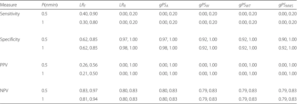
Table 7The 90th percentile confidence intervals for all performance measure estimates of each method for Scenario 6 in Table1
(corresponding to Fig.6)
Measure min(nk) LRF LRR gPSA gPSW gPSWT gPSMWS
Sensitivity 500 0.40, 0.90 0.00, 0.20 0.00, 0.20 0.00, 0.20 0.00, 0.20 0.00, 0.20
1000 0.50, 0.90 0.00, 0.30 0.00, 0.30 0.00, 0.20 0.00, 0.20 0.00, 0.20
Specificity 500 0.62, 0.85 0.97, 1.00 0.97, 1.00 0.92, 1.00 0.92, 1.00 0.90, 1.00
1000 0.57, 0.80 0.98, 1.00 0.98, 1.00 0.92, 1.00 0.95, 1.00 0.90, 1.00
PPV 500 0.26, 0.56 0.00, 1.00 0.00, 1.00 0.00, 1.00 0.00, 1.00 0.00, 1.00
1000 0.27, 0.53 0.00, 1.00 0.00, 1.00 0.00, 1.00 0.00, 1.00 0.00, 1.00
NPV 500 0.83, 0.97 0.80, 0.83 0.80, 0.83 0.79, 0.83 0.79, 0.83 0.79, 0.83
1000 0.84, 0.97 0.80, 0.85 0.80, 0.85 0.79, 0.83 0.79, 0.83 0.79, 0.83
min(nk)= minimum provider volume; PPV = positive predictive value; NPV = negative predictive value
Table 8The 90th percentile confidence intervals for all performance measure estimates of each method for Scenario 7 in Table1
(corresponding to Fig.7)
Measure P(nmin) LRF LRR gPSA gPSW gPSWT gPSMWS
Sensitivity 0.5 0.40, 0.90 0.00, 0.20 0.00, 0.20 0.00, 0.20 0.00, 0.20 0.00, 0.20
1 0.30, 0.80 0.00, 0.20 0.00, 0.20 0.00, 0.20 0.00, 0.20 0.00, 0.20
Specificity 0.5 0.62, 0.85 0.97, 1.00 0.97, 1.00 0.92, 1.00 0.92, 1.00 0.90, 1.00
1 0.62, 0.85 0.98, 1.00 0.98, 1.00 0.92, 1.00 0.92, 1.00 0.92, 1.00
PPV 0.5 0.26, 0.56 0.00, 1.00 0.00, 1.00 0.00, 1.00 0.00, 1.00 0.00, 1.00
1 0.21, 0.50 0.00, 1.00 0.00, 1.00 0.00, 1.00 0.00, 1.00 0.00, 1.00
NPV 0.5 0.83, 0.97 0.80, 0.83 0.80, 0.83 0.79, 0.83 0.79, 0.83 0.79, 0.83
1 0.81, 0.94 0.80, 0.83 0.80, 0.83 0.79, 0.83 0.79, 0.83 0.79, 0.83
Abbreviations
CABG: Coronary artery bypass grafting; PS: Propensity score; gPS: Generalized propensity score;LRF: fixed effects logistic regression;LRR: random effects logistic regression;gPSA: gPS case-mix adjustment;gPSW: gPS inverse probability weighting;gPSWT: gPS inverse probability weighting with trimming;
gPSMWS: gPS marginal mean weighting through stratification; mmw: Marginal mean weight; ppv: Positive predictive value; npv: Negative predictive value
Funding
RHH Groenwold was funded by the Netherlands Organization for Scientific Research (NWO-Vidi project 917.16.430). The funding body had no role in the design of the study, the collection, analysis, and interpretation of the data or the writing of the manuscript.
Availability of data and materials
Anonymized data used for the simulation study was provided by the Netherlands Association of Cardio-Thoracic Surgery. This anonymized data is not available to the public and cannot be published due to privacy concerns of the surgery centers included in the data set. Simulation programming code files are available upon reasonable request.
Authors’ contributions
TB performed the simulation study and wrote the majority of the manuscript. KR closely assisted with the design of the simulation study and the interpretation of the results. KM supervised the research, contributed to the design of the simulation study, and assisted in the assessment of societal impact of the research. RG was the initiator of the research project, closely supervised all technical analyses included in the paper and was a significant contributor to the decisions made for the analysis as well as the writing of the manuscript. All authors read and approved the final manuscript.
Ethics approval and consent to participate
According to the Central Committee on Research involving Human Subjects (CCMO), this type of study does not require approval from an ethics committee in the Netherlands. This study was approved by the data committee of the Netherlands Association of Cardio-Thoracic Surgery.
Competing interests
The authors declare that they have no competing interests.
Publisher’s Note
Springer Nature remains neutral with regard to jurisdictional claims in published maps and institutional affiliations.
Received: 16 October 2017 Accepted: 15 May 2018
References
1. Iezzoni LI, (ed). Risk Adjustment for Measuring Health Care Outcomes, 4th edn. Chicago: Health Administration Press; 2013.
2. Normand S-LT, Shahian DM. Statistical and clinical aspects of hospital outcomes profiling. Stat Sci. 2007;22(2):206–26.
3. Shahian DM, He X, Jacobs JP, Rankin JS, Peterson ED, Welke KF, Filardo G, Shewan CM, O’Brien SM. Issues in quality measurement: target population, risk adjustment, and ratings. Ann Thorac Surg. 2013;96(2): 718–26.
4. Englum BR, Saha-Chaudhuri P, Shahian DM, O’Brien SM, Brennan JM, Edwards FH, Peterson ED. The impact of high-risk cases on hospitals’ risk-adjusted coronary artery bypass grafting mortality rankings. Ann Thorac Surg. 2015;99(3):856–62.
5. Chassin MR, Hannan EL, DeBuono BA. Benefits and hazards of reporting medical outcomes publicly. N Engl J Med. 1996;334(6):394–8.
6. Austin PC, Alter DA, Tu JV. The use of fixed-and random-effects models for classifying hospitals as mortality outliers: a monte carlo assessment. Med Dec Making. 2003;23(6):526–39.
7. Jones HE, Spiegelhalter DJ. The identification of unusual health-care providers from a hierarchical model. Am Stat. 2011;65(3):154–63. 8. Shahian DM, Normand S-LT. What is a performance outlier? BMJ Qual Saf.
2015;24:95–9.
9. Mohammed MA, Deeks JJ, Girling AJ, Rudge G, Carmalt M, Stevens AJ, Lilford RJ. Evidence of methodological bias in hospital standardised
mortality ratios: retrospective database study of english hospitals. BMJ (Clin res ed.) 2009;338:1–8.
10. Glance LG, Dick AW, Osler TM, Li Y, Mukamel DB. Impact of changing the statistical methodology on hospital and surgical ranking: the case of the new york state cardiac surgery report card. Med Care. 2006;44(4):311–9. 11. Shahian DM, Wolf RE, Iezzoni LI. Variability in the measurement of
hospital-wide mortality rates. N Engl J Med. 2010;363(26):2530–9. 12. Bilimoria KY, Cohen ME, Merkow RP, Wang X, Bentrem DJ, Ingraham
AM, Richards K, Hall BL, Ko CY. Comparison of outlier identification methods in hospital surgical quality improvement programs. J Gastrointest Surg. 2010;14(10):1600–7.
13. Eijkenaar F, van Vliet RCJA. Performance profiling in primary care: does the choice of statistical model matter? Med Dec Making. 2014;34(2):192–205. 14. Krell RW, Hozain A, Kao LS, Dimick JB. Reliability of risk-adjusted
outcomes for profiling hospital surgical quality. JAMA Surg. 2014;149(5): 467–74.
15. Austin PC, Reeves MJ. Effect of provider volume on the accuracy of hospital report cards: a monte carlo study. Circ: Cardiovasc Qual Outcomes. 2014;7(2):299–305.
16. van Dishoeck A-M, Lingsma HF, Mackenbach JP, Steyerberg EW. Random variation and rankability of hospitals using outcome indicators. BMJ Qual Saf. 2011;20(10):869–74.
17. Landon BE, Normand S-lT, Blumenthal D, Daley J. Physician clinical performance assessment. JAMA. 2014;290(9):1183–9.
18. Huang I, Frangakis C, Dominici F, Diette GB, Wu AW. Application of a propensity score approach for risk adjustment in profiling multiple physician groups on asthma care. Health Serv Res. 2005;40(1):253–78. 19. Biondi-Zoccai G, Romagnoli E, Agostoni P, Capodanno D, Castagno D,
D’Ascenzo F, Sangiorgi G, Modena MG. Are propensity scores really superior to standard multivariable analysis? Contemp Clin Trials. 2011;32(5):731–40.
20. Stürmer T, Joshi M, Glynn RJ, Avorn J, Rothman KJ, Schneeweiss S. A review of the application of propensity score methods yielded increasing use, advantages in specific settings, but not substantially different estimates compared with conventional multivariable methods. J Clin Epidemiol. 2006;59(5):437–47.
21. Winkelmayer WC, Kurth T. Propensity scores: help or hype? Nephrol Dial Transplant. 2004;19(7):1671–3.
22. Austin PC. An introduction to propensity score methods for reducing the effects of confounding in observational studies. Multivar Behav Res. 2011;46(3):399–424.
23. Dehejia RH, Wahba S. Causal effects in nonexperimental studies: reevaluating the evaluation of training programs. J Am Stat Assoc. 1999;94(448):1053–62.
24. Martens EP, Pestman WR, de Boer A, Belitser SV, Klungel OH. Systematic differences in treatment effect estimates between propensity score methods and logistic regression. Int J Epidemiol. 2008;37(5):1142–7. 25. Rosenbaum PR, Rubin DB. The central role of the propensity score in
observational studies for causal effects. Biometrika. 1983;70(1):41–55. 26. Cepeda MS, Boston R, Farrar JT, Strom BL. Comparison of logistic
regression versus propensity score when the number of events is low and there are multiple confounders. Am J Epidemiol. 2003;158(3):280–7. 27. Kurth T, Walker AM, Glynn RJ, Chan KA, Gaziano JM, Berger K, Robins JM.
Results of multivariable logistic regression, propensity matching, propensity adjustment, and propensity-based weighting under conditions of nonuniform effect. Am J Epidemiol. 2006;163(3):262–70. 28. Brakenhoff TB, Moons KGM, Kluin J, Groenwold RHH. Investigating risk
adjustment methods for health care provider profiling when
observations are scarce or events rare. Health Serv Insights. 2018. In press. 29. Imbens GW. The role of the propensity score in estimating dose-response
functions. Biometrika. 2000;87(3):706–10.
30. Rassen JA, Shelat AA, Franklin JM, Glynn RJ, Solomon DH, Schneeweiss S. Matching by propensity score in cohort studies with three treatment groups. Epidemiol. 2013;24(3):401–9.
31. Feng P, Zhou X-H, Zou Q-M, Fan M-Y, Li X-S. Generalized propensity score for estimating the average treatment effect of multiple treatments. Stat Med. 2012;31(7):681–97.
32. Linden A, Uysal SD, Ryan A, Adams JL. Estimating causal effects for multivalued treatments: a comparison of approaches. Stat Med. 2015;35(4):534–52.
34. MacKenzie TA, Grunkemeier GL, Grunwald GK, O’Malley AJ, Bohn C, Wu Y, Malenka DJ. A primer on using shrinkage to compare in-hospital mortality between centers. Ann Thorac Surg. 2015;99(3):757–61. 35. Fedeli U, Brocco S, Alba N, Rosato R, Spolaore P. The choice between
different statistical approaches to risk-adjustment influenced the identification of outliers. J Clin Epidemiol. 2007;60(8):858–62. 36. Alexandrescu R, Bottle A, Jarman B, Aylin P. Classifying hospitals as
mortality outliers: Logistic versus hierarchical logistic models. J Med Syst. 2014;38(5):1–7.
37. Hubbard RA, Benjamin-Johnson R, Onega T, Smith-Bindman R, Zhu W, Fenton JJ. Classification accuracy of claims-based methods for identifying providers failing to meet performance targets. Stat Med. 2015;34(1): 93–105.
38. Racz MJ. Bayesian and frequentist methods for provider profiling using risk-adjusted assessments of medical outcomes. J Am Stat Assoc. 2010;105(489):48–58.
39. Yang X, Peng B, Chen R, Zhang Q, Zhu D, Zhang QJ, Xue F, Qi L. Statistical profiling methods with hierarchical logistic regression for healthcare providers with binary outcomes. J Appl Stat. 2013;41(1): 46–59.
40. Shahian DM, Normand S-LT, Torchiana DF, Lewis SM, Pastore JO, Kuntz RE, Dreyer PI. Cardiac surgery report cards: comprehensive review and statistical critique. Ann Thorac Surg. 2001;72:2155–68.
41. Imai K, van Dyk DA. Causal inference with general treatment regimes: generalizing the propensity score. J Am Stat Assoc. 2004;99(467):854–66. 42. Spreeuwenberg MD, Bartak A, Croon MA, Hagenaars JA, Busschbach
JJV, Andrea H, Twisk J, Stijnen T. The multiple propensity score as control for bias in the comparison of more than two treatment arms: an introduction from a case study in mental health. Med Care. 2010;48(2): 166–74.
43. Lee BK, Lessler J, Stuart EA. Weight trimming and propensity score weighting. PLoS ONE. 2011;6(3):1–6.
44. Hong G. Marginal mean weighting through stratification: a generalized method for evaluating multivalued and multiple treatments with nonexperimental data. Psychol Methods. 2012;17(1):44–60.
45. Linden A. Combining propensity score-based stratification and weighting to improve causal inference in the evaluation of health care interventions. J Eval Clin Pract. 2014;20(6):1065–71.
46. Yang S, Imbens GW, Cui Z, Faries D, Kadziola Z. Propensity score matching and subclassification in observational studies with multi-level treatments. Biometrics. 2014;72(4):1055–65.
47. Wang Y, Cai H, Li C, Jiang Z, Wang L, Song J, Xia J. Optimal caliper width for propensity score matching of three treatment groups: a monte carlo study. PloS ONE. 2013;8(12):1–7.
48. Austin PC. The relative ability of different propensity score methods to balance measured covariates between treated and untreated subjects in observational studies. Med Dec Making. 2009;29(6):661–77.
49. Lunceford JK, Davidian M. Stratification and weighting via the propensity score in estimation of causal treatment effects: a comparative study. Stat Med. 2004;23(19):2937–60.
50. R Core Team. R: a language and environment for statistical computing. Vienna; 2015.https://www.R-project.org.
51. Siregar S, Groenwold RHH, Versteegh MIM, Takkenberg JJM, Bots ML, van der Graaf Y, van Herwerden LA. Data resource profile: Adult cardiac surgery database of the netherlands association for cardio-thoracic surgery. Int J Epidemiol. 2013;42(1):142–9.
52. Siregar S, Groenwold RHH, Jansen EK, Bots ML, van der Graaf Y, van Herwerden LA. Limitations of ranking lists based on cardiac surgery mortality rates. Circ: Cardiovasc Qual Outcomes. 2012;5(3):403–9. 53. Roques F, Nashef SAM, Michel P, Gauducheau E, De Vincentiis C,
Baudet E, Cortina J, David M, Faichney A, Gavrielle F, Gams E, Harjula A, Jones MT, Pinna Pintor P, Salamon R, Thulin L. Risk factors and outcome in european cardiac surgery: Analysis of the euroscore multinational database of 19030 patients. Eur J Cardiothorac Surg. 1999;15(6):816–23. 54. Birkmeyer JD, Siewers AE. Hospital volume and surgical mortality in the
united states. N Engl J Med. 2002;346(15):1128–37.
55. Halm Ea, Lee C, Chassin MR. Is volume related to outcome in health care? a systematic review and methodologic critique of the literature. Ann Intern Med. 2002;137(6):511–20.
56. Cochran WG. The effectiveness of adjustment by subclassification in removing bias in observational studies. Biometrics. 1968;24(2):295–313.
57. Rosenbaum PR, Rubin DB. Reducing bias in observational studies using subclassification on the propensity score. J Am Stat Assoc. 1984;79(387): 516–24.
58. Bates D, Maechler M, Bolker B, Walker S. Fitting linear mixed-effects models using lme4. J Stat Softw. 2015;67(1):1–48.
59. Landsman V, Pfeiffer RM. On estimating average effects for multiple treatment groups. Stat Med. 2013;32(11):1829–41.