0 INTRODUCTION
Full-field measurement of displacement and strain has been made possible by modern digital camera technology and the development of algorithms in photogrammetry. The most popular approach is digital image correlation (DIC), based on maximising the correlation between reference and deformed
grey-intensity images [1] obtained from a pattern
of speckles applied on the surface of the test piece. DIC algorithms can be mainly classified into two categories [2]: local DIC algorithms known as
subset-based DIC [3] and global DIC algorithms known as
full-field DIC [4] to [8].
Subset DIC is generally based on square subsets of k×k pixels with shape functions applied to estimate a smooth displacement field across each subset. This generally leads to edge discontinuity, causing sensitivity to noise and can result in significant
measurement errors [9]. One way of overcoming this
problem is to increase the size of the subset. In this way measurement precision may be increased, but this is necessarily accompanied by a deterioration in spatial resolution brought about by making the subset larger
[10] to [13] – each subset has a single measurement
point, generally at its centre. Full-field or global DIC is regarded as being more robust than subset DIC to
image noise. However, its spatial resolution may also be degraded by the smoothing effect introduced by continuous constraints.
The literature on measurement precision and spatial resolution is extensive. For example, some
algorithms [14] to [16] are employed to generate
synthetic images that mimic real patterns of displacement in both Fourier [17] and spatial domains
[18]. Artificial displacements may be applied to a
piece of experimental speckle image [19] for the same purpose. It is straightforward to quantify precision by evaluating the noise level of the measured displacement in terms of standard deviation [7], [8] and [11]. However, the study of spatially fluctuating displacement fields [20] and [21] usually requires the evaluation of the spatial resolution of DIC algorithms, which is very difficult to implement experimentally. Bornert et al. [11] produced synthetic speckle images with superimposed planar sinusoidal displacements. Different spatial frequencies were applied to enable the study of the spatial resolution effectively in terms of statistical properties. The same approach was followed by Wittevrongel et al. [8] to help re-define the spatial resolution of local and global DIC algorithm. It allows a fair comparison of the performance between different types of DIC algorithms, i.e. the subset
DIC and a global DIC approach called p-DIC [8], by
Measurement Precision and Spatial Resolution
with Kriging Digital Image Correlation
Wang, D. – Mottershead, J.E.
Dezhi Wang1 – John E. Mottershead1,2,*
1 University of Liverpool, Centre for Engineering Dynamics, UK 2 University of Liverpool, Institute for Risk and Uncertainty, UK
The performance of a new global digital image correlation (DIC) approach known as Kriging DIC is assessed by comparison with the classical subset-based DIC through a standard evaluation procedure. This procedure employs synthetic images with imposed planar sinusoidal displacement fields of various spatial frequencies to quantify both the displacement measurement precision and the spatial resolution of DIC algorithms. The displacement precision and spatial resolution are re-defined in terms of two measures of discrepancy that have not been used before but are considered to give a better comparative assessment than was previously possible. The results are presented in graphical form to finally produce an evaluation of the relative performance of the different DIC approaches. These show that the Kriging DIC approach is robust to the measurement noise and has superior performance to the classical subset-based DIC in terms of both displacement measurement precision and spatial resolution. Furthermore, it is found that the best results are obtained when the discrepancy is measured in the normal direction, as opposed to the Y-direction for the quantification DIC performance.
Keywords: digital image correlation, Kriging regression, measurement precision, spatial resolution Highlights
• Two new measures of displacement discrepancy are used to redefine the measurement precision and spatial resolution for both local and global DIC.
considering the combination of precision and spatial resolution at the same time.
In this technology the classical definition of precision (also call displacement resolution) is the smallest change in the displacement field that can be readily measured and reflected in the measured displacement [7] and [22]. The spatial resolution is said to be the smallest distance between two independent
measurement points [7] and [22]. The spatial
resolution of subset-based DIC may be considered to be the subset size while the spatial resolution of global DIC depends on the number of measurements obtained within the region of interest (RoI). However, this classical definition is not applicable to global DIC since measurement points are correlated and the independence is not clearly defined. A practical definition of the spatial resolution was proposed by
Sutton [23] as one half of the period of the highest
frequency component that can be measured in the frequency band of the displacement data.
Spatial resolution is now generally understood to mean the half-period of the spatial frequency (the half wavelength) at which the measurement precision exceeds some chosen threshold. In a purely numerical test a planar unidirectional sinusoidal displacement is applied to a rectangular strip of speckles. Gaussian white noise is applied to represent measurement errors. Grey-level reference and deformed images are defined and the DIC estimate is compared statistically (usually in terms of the mean error and standard deviation) to the true sinusoid. The half-period spatial resolution is the minimum required to reconstruct the sinusoid without aliasing using the fast Fourier transform (FFT). This corresponds to the sampling rate, being twice the Nyquist frequency (i.e. the frequency of the sinusoid).
Generally for both the local and global DIC algorithms, a compromise has to be made between measurement precision and spatial resolution. An ideal DIC algorithm is expected to be able to achieve an excellent precision and an excellent spatial resolution at the same time [7] and [8]. Since the complexity of the sought displacement field is normally unknown before measurement, the optimal DIC algorithm for a specific application is not constant and relies on the trade-off between the detailed measurement of a displacement field and keeping the noise-induced error at a low level. In practice, a priori knowledge of the overall complexity of the displacement field can be quantified, for example, through finite element analysis [24]. In that case, the optimal DIC algorithm and parameters might be determined by performing simulated experiments [25].
Recently a new global DIC algorithm with
integrated Kriging regression [26] was developed by
the present authors. A Kriging regression model was integrated into the global DIC framework as a full-field shape function to formulate full-field displacement in a more accurate realisation of unknown true displacement fields. The lack of knowledge of the true displacement field was modelled by a Gaussian random process resulting in a Kriging model as a best linear unbiased prediction. A regularisation technique (in a global sense) was utilized to further improve the accuracy of Kriging model and to yield an approximation method to quantify control-point displacement errors. Furthermore, an updating strategy for the self-adaptive control grid was developed on the basis of the mean squared error (MSE) determined from the Kriging model. The proposed Kriging DIC approach showed excellent performance on displacement resolution and outperformed several other full-field DIC methods when using open-access experimental data. However, as discussed above, the performance of a DIC algorithm should be comprehensively validated through an examination of measurement precision and spatial resolution.
Thus in this study, a comparison is made between Kriging DIC and the classical subset-based DIC in terms of measurement precision and spatial resolution. This is carried out by using a series of synthetic speckle images imposed with planar sinusoidal displacements with various spatial frequencies. Apart from the use of different DIC algorithms, other parameters and schemes, e.g. grey-intensity interpolation, are the same in the comparison. In the sequel, the Kriging DIC algorithm is briefly introduced, the methodology for the comparison is explained and new improved definitions of precision and spatial resolutions are given. Finally, results are produced that illustrate the good performance of the Kriging DIC algorithm.
1 KRIGING DIC
Kriging DIC [26] is a new global DIC algorithm
with excellent robustness to image noise, good adaptation to displacement fields, and independent of user intervention. It is effective for a wide range of applications. A further validation of the performance of the method could lead to improvements in prospective applications and should be beneficial for further research. In the following, the details of Kriging DIC approach are very briefly introduced.
between images [3]. The matching criterion is normally interpreted in the form of minimising
the sum of squared differences (SSD) [27] of grey
intensities between two images. The SSD criterion may be written as
CSSD =
(
(
+ +)
−−
)
∫
arg min ( , ), ( , )
( , ) ,
g x u x z z v x z f x z
Θ Θ
2
d (1)
where Θ denotes the RoI in the first image. The
displacement
(
u x z v x z( , ),( )
,)
may be understood asthe optical flow of the speckle-pattern intensity from a
reference image f x z( , ) to its corresponding
deformed image g x z( , ) with x z, coordinates in
pixels. The whole RoI may be divided into a large number of small ‘subsets’ [7] (subset-based DIC) or be treated as a single large ‘subset’ (global DIC) to carry out the correlation.
In order to find a solution for the DIC correlation criterion, the displacement field of a subset or RoI may be modelled using a shape function with finite unknown parameters to be determined. For both global and local DIC approaches, the displacement field
(
u x z v x z( , ),( )
,)
can be approximated as a linearcombination of chosen basis functions of unknown parameters [7], [26] and [28] with finite dimension n, expressed as:
u x z x z p
v x z x z p
j u j n j v j n j j ( , ) ( , ) , ( , ) ( , ) , ≈ ≈ = =
∑
∑
µ µ 1 1 (2)where µj( , );x z j=1 2, ,,n are kernel functions and p p juj, vj; =1 2, ,,n are combination coefficients. The grey intensity image g x u x z z v x z
(
+ ( , ), + ( , ))
isan implicit function of
(
u x z v x z( , ),( )
,)
and thespatial-domain Newton-Raphson iteration [29] and
[30] is usually applied to solve the minimisation
problem.
As a global algorithm, Kriging DIC is implemented by applying a Kriging regression model as the global shape function to estimate the true displacement field w x z( , ) as a best linear unbiased
prediction (BLUP) [31], where
w x z( , )∈
{
u x z v x z( , ), ( , )}
represents thesingle-direction displacement field (i.e. either u x z( , ) or
v x z( , )). Specifically, w x z( , ) is modelled as a
realisation of a random function which combines a deterministic regression model and a zero-mean stochastic field [32]. Denoting w0=
[
w1,,wn]
T
as displacements of a set of chosen control points
x zj, j ,j , , , ,n
(
)
=1 2 the displacement responsew x z( , ) at an arbitrary untried location
( )
x z, can beformulated by the Kriging model in terms of a linear combination of the sample values w0 [33] and [26],
w x z j x z w
j n j ( , )= ( , ) = , =
∑
κ 1 0κκTw (3)
where the Kriging weights are given by,
κκ x z
x z
x z x
n , , , ,
( )
=(
)
= =(
( )
−(
)
× ×( )
− − − − −κ1 κ2 κ
1 1 1
1
T
R r C C R C
C R r c
T
T
( )
zz(
)
)
. (4)The matrix C and vector c contain
regression-function terms corresponding to the control points and the point of interest
( )
x z, respectively. In the present study the exponential (or Gaussian) kernel function,rjk =exp
(
−ϑx(
xj−xk)
−ϑz(
zj−zk)
)
, (5)is used to define the correlation between control points, in matrix R, and between the point of interest
x z,
( )
and each of the control points, in vector r( )
x z, . The Kriging weights are optimised by minimising the mean square (MSE) using the parameters Jx, Jz and a regularisation parameter that accounts for measurement imprecision at the control points [26]. This formulation relies on an assumption that the displacement function is smooth and continuous (i.e. without irregularities or discontinuities).Apart from the application of the Kriging shape function, Kriging DIC also has several special features which are absent from classical DIC algorithms. Based on the discussion in [26], some general remarks may be made as follows:
• Uncertainty in the Kriging DIC estimate is represented by a Gaussian random process with measurement errors incorporated into the correlation matrix.
• A global optimisation process results in the most probable estimate (rather than the best fit) – it does so automatically without user intervention. • Kriging DIC is capable of adapting to any
• The optimal number and distribution of control points can be achieved automatically through a self-adaptive updating process.
2 EXPERIMENTAL MEASUREMENT PRECISION AND SPATIAL RESOLUTION
In this section a procedure is explained which is essentially similar that described by Bornert et al. [11] and Wittevrongel et al. [8]. However, whereas in [8] the threshold on measurement precision is based only on the difference in amplitude between the imposed sinusoid and the corresponding measurement, in the present work a more complete measure of the discrepancy is used. We begin with a general measure of discrepancy, denoted by the vector
{ }
εi in=1. Without being specific it represents in some way the difference between the imposed sinusoid and measurement at the control points, i=1,,n, of the Kriging model. The statistics of error may then be defined in terms of the estimated mean and standard deviation (STD) as,εi i εi n
n
=
∑
=1 , (6)and σε= ε ε −
(
)
−(
)
= =∑
∑
n n n i i n i i n 2 1 1 21 , (7)
and the root mean squared error (RMSE) is given by,
RMS n
n i
ε = σε ε −
+ 1 2 2
. (8)
The unidirectional planar sinusoid imposed in on the rectangular speckle pattern defines the true displacement as, u A p x u x z = = sin , 2 0 π (9)
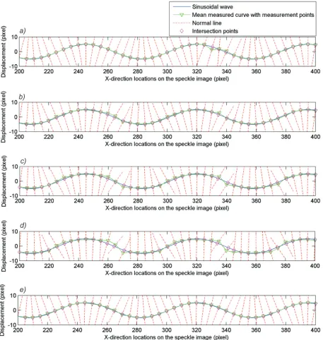
where A and p denote the amplitude and period. Examples of the imposed sinusoid and measured displacement are shown in Fig. 1 for subset-based and Kriging DIC. The sine wave has an amplitude 5 pixels, a period of 75 pixels and zero-mean Gaussian noise is added with a standard deviation 3 grey values. The deformed speckle pattern [8] and [11] is shown in Fig. 2. The red dashed lines shown in Fig. 1 are constructed normal to the measurement at the Kriging control points. This case illustrates one candidate measure of the discrepancy
{ }
εi in=1 given by the difference
between the measurement and the intersection of the normal with the sinusoid. Another possibility would
be to use the discrepancy measured only in the direction of the displacement (i.e. the Y-direction discrepancy), but in this case one would expect the discrepancy to be greater than that measured in the direction of the normal. The smaller the measure of discrepancy the better, and therefore normal measure is considered to be superior to the Y-direction measure. Of course, since the sinusoid is by definition a nonlinear function of x, it is necessary to iterate to determine the intersection precisely.
The displacement measurement precision and spatial resolution were defined in general terms in the Introduction. In the results presented here the spatial resolution is understood to be one half of the lowest spatial period in pixels at which the DIC measurement is able to reproduce the true displacement to within a
RMSε of 5 % or 1.5 % of the amplitude of the sinusoid.
The precision is defined as the standard deviation
σε (corresponding to the 5 % or 1.5 % discrepancy
on RMSε), measured in pixels in either the normal
direction or the Y-direction.
3 PERFORMANCE OF KRIGING DIC ALGORITHM
In this section, performance of the Kriging-DIC algorithm, in terms of the displacement precision and spatial resolution, is assessed by means of a comparison with the classical subset-based DIC algorithm. A series of images with different sinusoidal deformation fields are used to calculate the displacement precision and spatial resolution of both the subset-based DIC and the Kriging DIC. The sinusoidal displacement field cannot be perfectly reconstructed using polynomial shape functions and therefore provides a good test and a standard procedure for assessing the performance of DIC algorithms. In this study, the original displacement measurement is investigated, rather than strain which is a derived quantity obtained by post-processing.
The reference images are defined by an experimental speckle pattern while the parameters of the deformed images with sinusoidal displacement fields are shown in Table 1. A region of interest with uniformly distributed sample points (centres of subsets) is selected which contains several periods of the sinusoidal displacement. Both the subset-based DIC and Kriging DIC methods are applied to measure the displacements at the sample points and then calculate the Y-direction discrepancy and the normal discrepancy respectively. In both cases the displacement precision is quantified in terms of
standard deviation σε. The DIC algorithm parameters
Fig. 1. The normal discrepancy: a) subset DIC size 31×31, b) subset DIC size 41×41, c) subset DIC size 51×51, d) subset DIC size 61×61, e) 1st order Kriging DIC
squared differences (NSSD) criterion was instead of the classical SSD for reasons of increased robustness [34].
Table 1. Parameters of the sinusoidal deformed images
Parameter Value
Amplitude 5 pixels
Period 25 →25 200 pixels
Gaussian noise (standard deviation) 3 grey values
Table 2. Parameters of DIC algorithms
Subset-based DIC Kriging DIC
Criterion NSSD NSSD
Sample (control) points 31×10 31×10
Subset size 31 →10 61 (pixels)
Regression order 0, 1st and 2nd
Correlation function Exponential
Shape function 2nd-order
Intensity interpolation 6×6 bi-cubic 6×6 bi-cubic
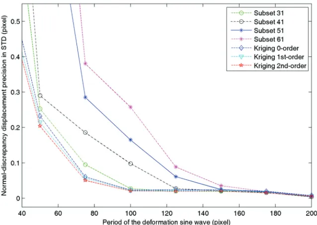
Fig. 3. The RMSE of the normal discrepancy in terms of the percentage (5 % and 1.5 %) of the sinusoidal amplitude vs the period of sinusoidal deformation
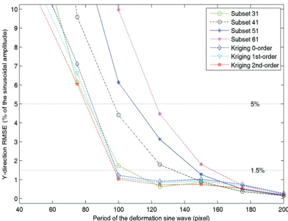
Fig. 5. The RMSE of the Y-direction discrepancy in terms of the percentage (5 % and 1.5 %) of the sinusoidal amplitude vs the period of sinusoidal deformation
Fig. 6. The displacement precision (STD of Y-direction discrepancy) vs the period of sinusoidal deformation
Figs. 3 and 4 and Figs. 5 and 6 show the root mean squared error (RMSE) and the standard deviation of the normal discrepancy and the Y-direction discrepancy respectively. As expected, the RMSE and the standard deviation both decrease as the period of the sinusoid increases. In Figs. 3 and 5 the 5 % and 1.5 % errors are shown and it is seen that the Kriging models with 0th, 1st and 2nd order regression polynomials are able
to accurately represent sinusoidal displacements with
low periods (high spatial frequency). The spatial resolution of a particular DIC code is given by half the period corresponding to the intersection of the RSME curve with the horizontal 5 % or 1.5 % line.
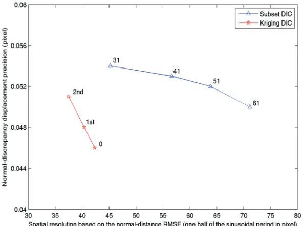
the same spatial resolution as the 31×31 pixel subset
DIC code. The equivalent Y-direction comparison is
presented in Figs. 9 and 10, where again the Kriging DIC approach produces improved results over the subset DIC code, but not such a great improvements
as is apparent from Figs. 7 and 8. The Y-direction
measurement tends to overestimate the error, which is better estimated using the normal direction
measure, and therefore the result shown in Figs. 7 and 8 is considered to represent a better performance comparison than in Figs. 9 and 10. It is clear also that increasing the order of regression in Kriging DIC enables a small improvement in spatial resolution to be achieved at considerable cost to measurement precision.
Fig. 7. Displacement precision vs spatial resolution (one half of the periods) based on the normal-discrepancy RMSE under the criterion of 5 % sinusoidal amplitude, for subset-based DIC using different subset sizes and Kriging DIC with different order regression functions
4 CONCLUSIONS
The performance of the Kriging DIC algorithm in terms of measurement precision and spatial resolution is considered in this study. A comparison is made between Kriging DIC and the classical subset-based DIC on the basis of a series of speckle images with
imposed sinusoidal deformation of various spatial frequencies. Two new measures of displacement discrepancy are used to redefine the measurement precision and spatial resolution for both local and global DIC. The difference between the true sinusoid and the measurement is determined most accurately when measured along the normal at the Kriging control
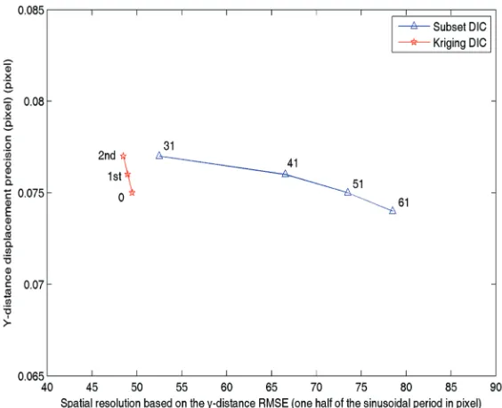
Fig. 9. Displacement precision vs spatial resolution based on the Y-direction RMSE under the criterion of 5 % sinusoidal amplitude, for subset-based DIC and Kriging DIC
points. This enables a better assessment to be made of the relative merits of different DIC algorithms. Results obtained using the RMSE criterion of 5 % and 1.5 % of the sinusoidal amplitude show Kriging DIC to be superior to classical sub-set based DIC in both displacement measurement precision and spatial resolution.
5 ACKNOWLEDGEMENTS
The authors wish to acknowledge the contribution of Lucas Wittevrongel in providing the sinusoidal deformation images used in this study. The first author acknowledges the support of the China Scholarship Council and the University of Liverpool.
6 REFERENCES
[1] Aster, R.C., Borchers, B., Thurber, C.H. (2005). Parameter Estimation and Inverse Problems. Academic Press, Amsterdam.
[2] Passieux, J.C., Bugarin, F., David, C., Perie, J.N., Robert, L. (2015). Multiscale displacement field measurement using digital image correlation: Application to the identification of elastic properties. Experimental Mechanics, vol. 55, no. 1, p.121-137, DOI:10.1007/s11340-014-9872-4.
[3] Sutton, M.A., Orteu, J.J., Schreier, H.W. (2009). Image Correlation for Shape, Motion and Deformation Measurements: Basic Concepts, Theory and Applications. Springer, New York.
[4] Rethore, J., Hild, F., Roux, S. (2007). Shear-band capturing using a multiscale extended digital image correlation technique. Computer Methods in Applied Mechanics and Engineering, vol. 196, no. 49-52, p. 5016-5030,
DOI:10.1016/j.cma.2007.06.019.
[5] Wagne, B., Roux, S., Hild, F. (2002). Spectral approach to displacement evaluation from image analysis. European Physical Journal - Applied Physics, vol. 17, no. 3, p. 247-252,
DOI:10.1051/epjap:2002019.
[6] Cheng, P., Sutton, M.A., Schreier, H.W., McNeill, S.R. (2002). Full-field speckle pattern image correlation with B-spline deformation function. Experimental Mechanics, vol. 42, no. 3, p. 344-352, DOI:10.1007/BF02410992.
[7] Mortazavi, F. (2013). Development of a Global Digital Image Correlation Approach for Fast High-Resolution Displacement Measurements. PhD thesis, École Polytechnique de Montréal, Montreal.
[8] Wittevrongel, L., Lava, P., Lomov, S.V., Debruyne, D. (2015). A self adaptive global digital image correlation algorithm. Experimental Mechanics, vol. 55, no. 2, p. 361-378,
DOI:10.1007/s11340-014-9946-3.
[9] Hild, F., Roux, S. (2012). Comparison of local and global approaches to digital image correlation. Experimental Mechanics, vol. 52, no. 9, p. 1503-1519, DOI:10.1007/ s11340-012-9603-7.
[10] Hild, F., Roux, S. (2006). Digital image correlation: from displacement measurement to identification of elastic
properties - a review. Strain, vol. 42, no. 2, p. 69-80,
DOI:10.1111/j.1475-1305.2006.00258.x.
[11] Bornert, M., Brémand, F., Doumalin, P., Dupre, J.-C., Fazzini, M., Grédiac, M., Hild, F., Mistou, S., Molimard, J., Orteu, J.-J.. Robert, L., Surrel, Y., Vacher, P., Wattrisse, B. (2009). Assessment of digital image correlation measurement errors: Methodology and results. Experimental Mechanics, vol. 49, no. 3, p. 353-370, DOI:10.1007/s11340-008-9204-7.
[12] Triconnet, K., Derrien, K., Hild, F., Baptiste, D. (2009). Parameter choice for optimized digital image correlation. Optics and Lasers in Engineering, vol. 47, no. 6, p. 728-737,
DOI:10.1016/j.optlaseng.2008.10.015.
[13] Besnard, G., Hild, F., Roux, S. (2006). “Finite-Element” displacement fields analysis from digital images: Application to portevin-le châtelier bands. Experimental Mechanics, vol. 46, no. 6, p. 789-803, DOI:10.1007/s11340-006-9824-8.
[14] Zhou, P., Goodson, K.E. (2001). Subpixel displacement and deformation gradient measurement using digital image/ speckle correlation (DISC). Optical Engineering, vol. 40, no. 8 p. 1613-1620, DOI:10.1117/1.1387992.
[15] Perlin, K. (1985). An image synthesizer. Proceedings of the SIGGRAPH Conference, San Francisco, p. 287-296,
DOI:10.1145/325165.325247.
[16] Orteu, J.-J., Garcia, D., Robert, L., Bugarin, F. (2006). A speckle texture image generator. Proceedings of the Speckle International Conference, Nîmes, DOI:10.1117/12.695280.
[17] Schreier, H.W., Braasch, J.R., Sutton, M.A. (2000). Systematic errors in digital image correlation caused by intensity interpolation. Optical Engineering, vol. 39, no. 11, p. 2915-2921, DOI:10.1117/1.1314593.
[18] Pan, B., Xie, H.-M., Xu, B.-Q., Dai, F.-L. (2006). Performance of sub-pixel registration algorithms in digital image correlation. Measurement Science and Technology, vol. 17, no. 6, p. 1615-1621, DOI:10.1088/0957-0233/17/6/045.
[19] Bergonnier, S., Hild, F., Roux, S. (2005). Digital image correlation used for mechanical tests on crimped glass wool samples. Journal of Strain Analysis for Engineering Design, vol. 40, no. 2, p. 185-198, DOI:10.1243/030932405X7773.
[20] Schreier, H.W., Sutton, M.A. (2002). Systematic errors in digital image correlation due to undermatched subset shape functions. Experimental Mechanics, vol. 42, no. 3,p. 303-310,
DOI:10.1007/BF02410987.
[21] Réthoré, J., Hild, F., Roux, S. (2008). Extended digital image correlation with crack shape optimization. International Journal for Numerical Methods in Engineering, vol. 73, no. 2, p. 248-272, DOI:10.1002/nme.2070.
[22] De Bievre, P. (2009). The 2007 International Vocabulary of Metrology (VIM), JCGM 200:2008 [ISO/IEC Guide 99]: Meeting the need for intercontinentally understood concepts and their associated intercontinentally agreed terms. Clinical Biochemistry, vol. 42, no. 4-5p. 246-248, DOI:10.1016/j. clinbiochem.2008.09.007.
[23] Sutton, M.A. (2010). ASTM E2208 Standard Guide for evaluating Non-Contacting Optical Strain Measurement Systems. ASTM International, West Conshohocken,
DOI:10.1520/E2208-02R10E01.
using deformation fields generated by plastic FEA. Optics and Lasers in Engineering, vol. 47, no. 7-8, p. 747-753,
DOI:10.1016/j.optlaseng.2009.03.007.
[25] Canal, L.P., González, C., Molina-Aldareguía, J.M., Segurado, J., LLorca, J. (2012). Application of digital image correlation at the microscale in fiber-reinforced composites. Composites Part A:Applied Science and Manufacturing, vol. 43, no. 10, p. 1630-1638, DOI:10.1016/j.compositesa.2011.07.014.
[26] Wang, D.Z., DiazDelaO, F.A., Wang, W.Z., Mottershead, J.E. (2015). Full-field digital image correlation with Kriging regression. Optics and Lasers in Engineering, vol. 67, p. 105-115, DOI:10.1016/j.optlaseng.2014.11.004.
[27] Chen, D.J., Chiang, F.P., Tan, Y.S., Don, H.S. (1993). Digital speckle-displacement measurement using a complex spectrum method. Applied Optics, vol. 32, no. 11, p. 1839-1849, DOI:10.1364/AO.32.001839.
[28] Hild, F., Roux, S. (2012). Comparison of local and global approaches to digital image correlation. Experimental Mechanics, vol. 52, no. 9, p. 1503-1519, DOI:10.1007/ s11340-012-9603-7.
[29] Bruck, H.A., McNeill, S.R., Sutton, M.A., Peters, W.H. (1989). Digital image correlation using Newton-Raphson method of
partial differential correction. Experimental Mechanics, vol. 29, no. 3, p. 261-267, DOI:10.1007/BF02321405.
[30] Vendroux, G., Knauss, W.G. (1998). Submicron deformation field measurements: Part 2. Improved digital image correlation. Experimental Mechanics, vol. 38, no. 2 p. 86-92,
DOI:10.1007/BF02321649.
[31] Matheron, G. (1993). Principles of geostatistics. Economic Geology, vol. 58, no. 8, p. 1246-1266, DOI:10.2113/ gsecongeo.58.8.1246.
[32] Sacks, J., Welch, W.J., Mitchell, T.J., Wynn, H.P. (1989). Design and analysis of computer experiments. Statistical Science, vol. 4, no. 4, p. 409-435, DOI:10.1214/ss/1177012413.
[33] Wackernagel, H. (1998). Kriging Weights in Multivariate Geostatistics: An Introduction with Applications. Springer Berlin, Heidelberg, p. 93-99, DOI:10.1007/978-3-662-03550-4.