Bayesian Hierarchical Spatial-Temporal Models for Wind Prediction

(1)

Chen, Li. Bayesian Hierarchical Spatial-Temporal Models for Wind Prediction. (Under the direction of Dr. Montserrat Fuentes and Dr. Jerry M. Davis).

(2)

by

Li Chen

A dissertation submitted to the Graduate Faculty of North Carolina State University

in partial satisfaction of the requirements for the Degree of

Doctor of Philosophy

Department of Statistics

Raleigh

2004

Approved By:

Dr. David A. Dickey Dr. Sujit K. Ghosh

Dr. Gary M. Lackmann Dr. John F. Monahan

(3)

(4)

Biography

(5)

Acknowledgements

I would like to thank the members of my advisory committee for their advice and support during the preparation of my dissertation.

I am extremely grateful for having Dr. Montserrat Fuentes as my advisor. Her en-thusiasm, knowledgeable guidance, and constant support, including financial support, have meant a tremendous amount to me. She is not only an excellent researcher who imposes the highest standards on her academic work, but also an outstanding advisor who provides continuing encouragement for her students. I thank her for her encouragement to become an independent researcher, and I also admire her tireless energy and her devotion to her professional career.

I am also extremely grateful to Dr. Jerry M. Davis, my co-advisor, for his endless patience, direction and time. I am very thankful to him for his careful reading of my drafts and for his insightful comments that have helped me to understand the material better. He has not only been helpful in answering my questions but also helped me with his kindness and encouragement in everyday life.

Thanks to Dr. Dave A. Dickey for his advice and encouragement during my work on my dissertation. Thanks to Dr. Sujit K. Ghosh for his valuable comments on the Bayesian methods. Thanks to Dr. Gary M. Lackmann for many enjoyable and helpful discussions on meteorology. Thanks to Dr. John F. Monahan for his helpful questions and suggestions that have helped me to present the material better. I also would like to thank Dr. Pantula, Dr. Swallow and all my professors, and Terry Byron for all their help and encouragement over these past 4 years.

(6)

List of Figures

1.1 The location of the Chesapeake Bay. . . 2

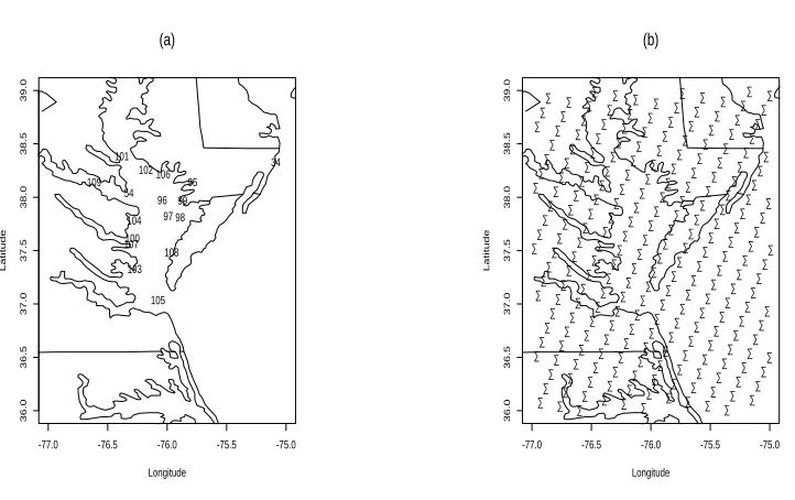
1.2 Location maps. . . 5

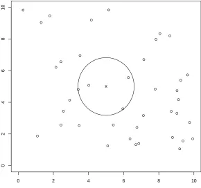
2.1 MWRRK. “x” indicates the predict location. . . 17

2.2 MCSTK. “x” indicates the predict point. . . 18

3.1 The contour plot for separable covariance S1. . . 33

3.2 The contour plot for nonseparable covariance N1. . . 33

3.5 The contour plot for a separable spatial-temporal covariance. . . 38

3.6 The contour plot for a nonseparable spatial-temporal covariance. . . 40

3.7 Contour plots for some nonseparable spatial-temporal covariances. . . 41

4.1 The general modeling framework. . . 53

5.1 The location map of monitoring sites. . . 65

5.2 Grid for MM5 output. . . 66

5.3 Wind field map from MM5 model forecast. . . 67

5.4 Subregions of stationarity. . . 69

5.5 The time series of wind speed has similar structure over space within each subregion. . . 71

5.6 The spatial process of wind speed has same pattern over time within each subregion except for subregion 4. . . 72

5.7 Spatial-temporal trend for wind speed. . . 73

5.8 Empirical covariance. . . 75

5.9 Posterior for sill. . . 77

5.10 Posterior for spatial range. . . 78

5.11 Posterior for conversion parameter. . . 79

5.12 Posterior for smoothness parameter. . . 80

5.13 Bayesian covariance. . . 81

5.14 MM5 model evaluation at 12pm on July 21, 2002. . . 82

(9)

5.16 MM5 model evaluation at 6pm on July 21, 2002. . . 84

5.17 Original MM5 output wind speed at 12pm on July 21, 2002. . . 86

5.18 Improved wind speed by combing data at 12pm on July 21, 2002 . . . 87

5.20 Improved wind speed by combing data at 3pm on July 21, 2002 . . . 89

(10)

List of Tables

1.1 Information of monitoring locations . . . 6

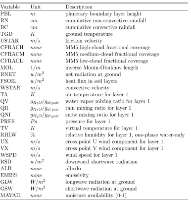
1.2 48 variables from MM5 model output. . . 8

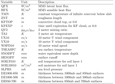
1.3 48 variables from MM5 model output (continued). . . 9

2.1 Hierarchical model by Wikle, Berliner, and Cressie (1998). . . 21

3.1 Separable covariance models. . . 31

3.2 Nonseparable covariance models. . . 31

4.1 Priors for the parameters in σ2(s) . . . 61

5.1 The posterior distribution for ²i. . . . 76

5.2 The posterior means for covariance parameters. . . 81

(11)

Chapter 1

Introduction

1.1 Motivation

The location of the Chesapeake Bay is shown by the bold box in Figure 1.1. To forecast the wind fields over the Chesapeake Bay is of long-standing interest, since the wind field in such a location is composed of many features that are spatially and temporally complex in nature, which makes for a very challenging forecasting problem. Despite the challenge, obtaining accurate wind field forecasts in the coastal zone is also critical to recre-ational interests, e.g., sailing, fishing and wind surfing; commercial interests, e.g., shipping and aviation; and environmental problems such as coastal erosion impacts. Increased em-phasis on homeland security issues provides an additional incentive for developing accurate forecasts of the coastal wind fields; forecast of chemical or biological emissions is critically dependent upon accurate prediction of near-surface wind speed and direction.

(12)

South Carolina North Carolina

Virginia West Virginia

Pennsylvania

Maryland New Jersey

(13)

addition, over the water surface persistent evaporation acts to lower the temperature of the air over the water surface in comparison to that over the land surface. Differences in the specific heats of water and soil also play a role, especially during the cooling cycle which begins in the evening hours. During the day, the land heats more quickly than the adjacent water, and the intensive heating of the air above produces a shallow thermal low. The air over the water remains cooler than the air over the land; hence, a shallow thermal high exists above the water. The overall effect of this pressure distribution is a sea breeze that blows from the sea toward the land within several kilometers of the coast. At night, the land cools more quickly than the water. The air above the land becomes cooler than the air over the water. With higher surface pressure now over the land, the wind reverses and becomes a land breeze which flows from the land toward the water (1). These effects lead to fundamental differences in heat flux between the two surfaces. As a result, the formation of a thermal internal boundary layer often takes place. Another result of these processes is that the stability regimes over water can differ greatly from those over land. Even the larger scale processes associated with these differences between the land boundary layer and marine boundary layer are difficult for a mesoscale model to capture.

(14)

reso-lution (e.g., 4 km) grid spacing. The ability of NWP models to represent coastal wind fields is limited even when the models are run at very high resolution, owing to limitations in the ability of these models to parameterize sub-grid scale process (19). Moreover, the lack of a dense observing network over coastal waters precludes accurate high-resolution initial conditions for atmospheric models.

Currently, Jay Titlow of WeatherFlow Enterprises uses the output from NCEP models as one component in his efforts to provide detailed wind field forecasts over the Chesapeake Bay. Titlow does not use a formal model (either dynamical, statistical, or a combination of the two) to produce the forecast. He mentally integrates the informa-tion which comes from a variety of sources along with an intelligence-system that he has developed, based on his forecasting experience, to produce the wind field forecast. Any pro-cedure that would make these meteorological model output wind fields more useful to him and others like him would be of great benefit to recreational interests, commercial interests and environmental interests.

Our main objective is to develop a statistical model which is capable of evaluating the mesoscale numerical model and providing reliable wind field maps over the Chesapeake Bay during the period of weak synoptic scale forcing.

1.2 Description of data

(15)

Longitude

Latitude

-77.0 -76.5 -76.0 -75.5 -75.0

36.0 36.5 37.0 37.5 38.0 38.5 39.0 105 106 109 101 99 107 104 98 102 103 34 54 95 108 96 97 100 (a) Longitude Latitude

-77.0 -76.5 -76.0 -75.5 -75.0

36.0 36.5 37.0 37.5 38.0 38.5 39.0 • • _• • _• • _• • • • _• • _• • _• • _• • _• • _• • _• • • _• • • _• • _• • _• • • _• • • _• • _• • _• • • _• • • _• • • _• • _• • • _• • _• • • _• • • _• • _• • • _• • _• • _• • _• • _• • • _• • _• • _• • _• • _• • _• • _• • _• • • _• • _• • • _• • • _• • • _• • _• • _• • _• • _• • _• • • _• • _• • _• • • _• • • _• • _• • _• • _• • • • _• • • _• • _• • _• • _• • _• • • _• • • _• • _• • • • • _• • • _• • • _• • _• • • • _• • • _• • _• • • _• • • _• • _• • _• • _• • _• • • • _• • • _• • _• • _• • _• • _• • _• • • _• • _• • • _• • _• • • _• • • _• • _• • • _• • _• • _• • _• • • _• • • _• • _• (b)

Figure 1.2: Location maps.

could be applied to meteorological model output. Limited data collection was continued into the summer of 2002. The criterion of weakly forced conditions was better met during the study period in 2002 than in 2001. The data from the 2002 period are used in analysis. During this period both observed data and MM5 (Penn State University/National Center for Atmospheric Research Mesoscale Model Version 5) output fields are available.

The observed data from the field experiment were measured hourly at 17 stations. These 17 stations are represented by the number in Figure 1.2 (a). The information of these 17 monitoring stations is given in the Table 1.1. At each station, the anemometer was at a different height above ground level. It varied from 9 meters to 18 meters. The observed data include not only the wind but also other weather information such as air temperature, pressure and humidity. The advantage of using the data from the experiment is that these special supplementary observed wind data were not integrated into the NCEP analysis used to initialize MM5, so that the MM5 model output and the observed wind data are independent.

(16)

Location ID Lattitude Longitude Sensor Height Land/Water

Ocean City KX034 38.328 75.086 15 water

Point Lookout KX054 38.04 76.322 15 land

Raccoon Point KX095 38.141 75.785 9 water

Smith Island KX096 37.974 76.041 10 land

Tangier Island KX097 37.823 75.991 17 land

Onancock KX098 37.813 75.89 12 land

Crisfield KX099 37.97 75.87 12 water

Windmill Point KX100 37.616 76.291 11 land

Cove Point KX101 38.384 76.382 13 land

Lower Hooper Island KX102 38.258 76.179 10 land

New Point Comfort KX103 37.328 76.273 15 land

Great Wicomico Light KX104 37.783 76.277 12 water

3rd Island CBBT KX105 37.036 76.077 15 land

Bishop’s Head KX106 38.217 76.033 18 land

Deltaville KX107 37.562 76.301 9 water

Silver Beach KX108 37.485 75.962 14 water

Coles Point KX109 38.142 76.614 9 water

(17)

because it is similar to the finest mesh produced by operational models run at the NCEP, and based on the discussion with Jay Titlow at WeatherFlow Inc. The MM5 model output has 48 variables (see Table 1.2 and Table 1.3) over 17 layers. The 10 meter wind fields were used for analysis.

1.3 Objectives

Our main objective is to develop a statistical model which is capable of statis-tically evaluating wind fields from MM5 and providing reliable wind field maps over the Chesapeake Bay.

The objective comparison between numerical model output and observed data provides a mean for assessing numerical model performance. However, it is not reasonable to compare them directly, since the numerical model output usually has a different spa-tial/temporal scale compared with observed data. The MM5 model output is grided over regular spatial cells, while data from the field experiment are point observations measured at the irregular spaced monitoring sites. These various data fields have different spatial scales. The hierarchical Bayesian approach is ideal for this application because it provides a mechanism for combining data from different resources with different spatial/temporal resolution, and it also provides a natural framework in which it is possible to include sci-entific knowledge in the model. The strategy is based on the formulation of three primary hierarchical stages:

• Stage 1. Data model: [data|underlying true process,parameters],

• Stage 2. Process model: [underlying true process|parameters],

• Stage 3. Prior: [parameters],

(18)

Variable Unit Description

PBL m planetary boundary layer height

RN cm cumulative non-convective rainfall

RC cm cumulative convective rainfall

TGD K ground temperature

USTAR m/s friction velocity

CFRACH none MM5 high-cloud fractional coverage CFRACM none MM5 medium-cloud fractional coverage CFRACL none MM5 low-cloud fractional coverage

MOL 1/m inverse Monin-Obukhov length

RNET w/m2 net radiation at ground FSOIL w/m2 heat flux in soil layers

WSTAR m/s convective velocity

TA K air temperature for layer 1

QV gH2O/gdryair water vapor mixing ratio for layer 1 QR gH2O/gdryair rain mixing ratio for layer 1

QNI gH₂O/gdryair snow mixing ratio for layer 1

PRES P a pressure for layer 1

TV K virtual temperature for layer 1

RHLW % relative humidity for layer 1, one-phase water-only UX m/s cross point U wind component for layer 1

VX m/s cross point V wind component for layer 1

WSPD m/s wind speed for layer 1

RSD w/m2 downward shortwave radiation

ALB none albedo

EMISS none emissivity

GLW W/m2 longwave radiation at ground GSW W/m2 shortwave radiation at ground MAVAIL none moisture availability (0-1)

(19)

Variable Unit Description

QFX W/m2 MM5 latent heat flux

HFX W/m2 MM5 sensible heat flux

TMN K constant temperature of infinite reservoir below slab

ZNT m roughness length

KFTOP m convective cloud top, or 0.0

KFEXP s time until expiration for KF cloud, or 0.0 QV2 gH2O/gair 2 meter mixing ratio

TA2 K 2 meter air temperature

UX10 m/s 10 meter U wind component

VX10 m/s 10 meter V wind component

WSPD10 m/s 10 meter wind speed

TSEASFC K sea surface temperature SNODPT mm water equivalent snow depth

SRNOFF mm surface runoff

SOILT010 K soil temperature for soil layer 1 SOILM010 m3/m3 soil moisture for soil layer 1

SLPRS mb sea level pressure

DZ1000-850 m thickness between 1000mb and 850mb surfaces DZ1000-500 m thickness between 1000mb and 500mb surfaces DZ850-700 m thickness between 850mb and 700mb surfaces

(20)

of the appropriate conditional distributions that may be motivated physically.

Bayesian analysis relies on the posterior distribution of the process of interest and the parameters given the data: [underlying true process,parameters|data]. This distribu-tion is propordistribu-tional to the product of the component distribudistribu-tions:

[data|underlying true process,parameters][underlying true process|parameters][parameters].

(21)

Chapter 2

Spatial-Temporal Processes

2.1 Introduction of spatial-temporal processes

Environmental data usually have both spatial and temporal components. For ex-ample, MM5 model output were generated at regular girds over regular time intervals, say every hour. Thus the data analysis has to take into account the spatial dependence among the grid cells, but also that the model output at each grid cell is not independent over time but forms a time series. In other words, one must take account of temporal correlations as well as spatial correlations. Therefore, it is essential to have statistical models to describe how the data vary across space and time.

Following 6), the data

{(Z(x₁,i, ti), . . . , Z(xni,i, ti)) :i= 1, . . . , m} (2.1) are assumed to be a finite sample of the stochastic process

{Z(x, t) :x∈D(t);t∈T}, (2.2) where the domain D(t) ⊂Rd may vary with time and T ⊂ R. Usually ni =n, D(t) ≡D and T = 1,2, . . ..

(22)

(1) E{Z(x, t)}=µ, whereµ is a constant;

(2) and cov{Z(x+h, t+u), Z(x, t)}=C(h, u)<∞, whereh∈Rd and u∈R,

then the process (2.2) is a weakly stationary spatial-temporal process. It is also called a second-order stationary spatial-temporal process.

Thus the covariance of Z, which is weakly stationary, depends only on the separa-tion vector (h, u). Define s = (x, t)∈Rd+1 _{to simplify the notation and write the} spatial-temporal process as Z(s). If Z(s) is weakly stationary, cov{Z(s₁), Z(s₂)} = C(s₁ −s₂), whereC(·) is positive definite and defined onRd+1. Positive definite means

N

X

i=1 N

X

j=1

aiajC(si−sj)≥0

for all finiteN, alls₁, . . . ,sN ∈D×T ⊂Rd+1 and all reala₁, . . . , aN. IfC(s1−s2) depends on (s₁−s₂) only through the Euclidean distance|s₁−s₂|, then Z(s) is isotropic.

Weak stationarity describes the property of shift invariance. A stronger form of shift invariance is strong stationarity.

Definition 2.1.2 (Strong Stationarity). A processZ(s) is strongly stationary if all of its finite dimensional distribution functions are shift invariant. That is, for any finite N and domainD×T, with{s,s₁, . . . ,sN} ⊆D×T and z1, . . . , zN ∈R then

P(Z(s₁+s)≤z₁, . . . , Z(sN +s)≤zN) =P(Z(s1)≤z1, . . . , Z(sN)≤zN).

Gaussian with finite second moment means strong stationarity. In general, strong stationarity implies weak stationarity, but the reverse is not true. For what follows, we work with weak stationarity and the wordstationaryrefers to weakly stationary.

Definition 2.1.3 (Separability). If the covariance of process (2.2) can be written as

cov{Z(s₁), Z(s₂)}= cov{Z(x₁, t₁), Z(x₂, t₂)}=CS(x1,x2)CT(t1, t2),

(23)

If we represent the data from a separable spatial-temporal process in the following vector form

Z= (Z(x₁, t₁),· · · , Z(xn, t₁),· · · , Z(x₁, tm),· · ·, Z(xn, tm))T,

then the separable spatial-temporal covariance matrix, Σ,can be written as the Kronecker product of a covariance matrix for time only with one for space only,

Σ = ΣT ⊗ΣS,

where ΣT is a m×m temporal covariance matrix and ΣS is a n×n spatial covariance matrix. The Kronecker product of two matricesV = (vij)m×m and U = (uij)n×n is defined as

V ⊗U =

    

v₁₁U . . . v₁mU ..

. . .. ...

vm1U . . . vmmU

    

mn×mn.

An advantage of a separable covariance is the great benefit for computation, because the inverse of Σ can be computed as

(Σ)−1 = (ΣT ⊗ΣS)−1= (ΣT)−1⊗(ΣS)−1,

and the determinant of Σ is given by

|Σ|=|ΣT ⊗ΣS|=|ΣT|n|ΣS|m.

Moreover, many techniques that have been developed and successfully used in time series analysis and geostatistics are available to this subclass of separable spatial-temporal pro-cesses.

From the definition of separability, we know that a separable process may or may not to be stationary. If a spatial-temporal process is separable and stationary, then

cov{Z(x₁, t₁), Z(x₂, t₂)}=CS(x1−x2)CT(t1−t2) =CS(h)CT(u),

(24)

The generic space-time problem is to use data (2.1) to predict Z(x₀, t₀) where x₀ ∈D and t₀ ∈ T. In the next section, we review some approaches to modeling spatial-temporal processes.

2.2 Recent approaches to spatial-temporal processes

The classical geostatistics approach is based on spatial processes which are sta-tionary , but it is widely recognized that real environmental processes are rarely stasta-tionary. In recent years, many methods for modeling nonstationary spatial processes have been developed. 29) present a nonparametric estimation procedure for nonstationary spatial covariance structure . The maximum likelihood approach is developed by 22) and 30). 13) introduces a moving-window kriging technique. 17) propose an alternative model to account for a nonstationary spatial covariance function, which is based on a moving aver-age specification of a Gaussian process. This spatial model allows the spatial dependence structure to vary as a function of location. 9) introduce a new class of nonstationary pro-cesses which is based on the convolution of local stationary propro-cesses. In contrast to a “moving-window” approach, this model has the advantage that it is simultaneously defined everywhere. Also 24) and 18) develop methods that extend the empirical orthogonal func-tions (EOF) approach which is popular among atmospheric scientists in the eighties and in the early nineties .

(25)

and hence its determinant and inverse are easily determinable. However, in real applications spatial-temporal processes are rarely separable and stationary.

The following subsections introduce some techniques for space-time process mod-eling. They are the maximum likelihood method, the moving window method and the Bayesian method. Some spatial-temporal covariance models are briefly reviewed too.

2.2.1 Maximum likelihood method

22) present a maximum likelihood approach to model multivariate spatial-temporal data when the sites are sparse but the time series is long.

Consider models for an m-variable spatial-temporal process, Z=Z(x, t), Z∈Rm where the locationxis in some domain of interestD⊂Rp _and_t_{indexes time. Then}_Z_may be written as

Z(x, t) =µ(x, t) +²(x, t) (2.3) where E(Z(x, t)) = µ(x, t), the set of m trend surfaces, and ² is a mean zero second-order stationary spatial-temporal Gaussian process with covariance Σ. Since the data in Mardia and Goodall’s application are equally spaced in time, they generalize the repeated measurements model, withN vectors of observations at each site, to a fully-factored model

Σ = ΣT SV = ΣT ⊗ΣS⊗ΣV

where theN ×N covariance matrix ΣT is from a temporal process. Σ is the notation for a generic covariance, and subscripts T, S, V denote temporal, spatial and multi-variate components.

(26)

simplified by assuming the same form for the trend surface, which means µ(x) =βtf. f is a polynomial function of spatial locations with coefficients β. For covariance, they impose the conditions of stationarity and spatial isotropy. The maximum likelihood estimation is carried out by an iterative algorithm. Then multivariable prediction is done by plugging in the maximum likelihood estimates. They also discuss the transformation to stationary isotropic spatial covariance using a complete deformation from the “geographic” space to the new “ isotropic” space.

Mardia and Goodall extend the multivariable spatial model to the case where a temporal variation is included. By using the factored model, they basically assume a sep-arable model for space-time covariance., which is not always the case in application. The approach should have the ability to take into account space-time dependency.

2.2.2 Moving window method

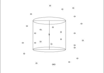
13) presents a method for prediction under spatial nonstationarity. He called this method “moving-window regression residual kriging” (MWRRK). He then extends the method to the nonstationary spatial-temporal case (14 14, 15). In the spatial case, the method simply restricts the estimation and prediction procedure to the collection of sample locations within a circular subregion, as a window, centered at each point of prediction, which is illustrated in Figure 2.1. For spatial-temporal case, the restriction is to sample points within a cylinder. The center of the cylinder is the prediction point s₀ = (x₀, t₀). The cylinder is constructed as follows. First, choose observations within a time window (t₀ − mT

(27)

0 2 4 6 8 10

02468

1

0

x

(28)

x

o.

o

oo

o

(29)

MCSTK consists of a two stage nonlinear regression procedure similar to that de-scribed by Cressie (1993, p. 22-24) for a two stage approach to linear estimated generalized least squares(EGLS).

The regression model in each prediction cylinder is

Y(s) =µ(s, β) +ψ(µ(s, β),s)R(s),

wheres= (x, t) is the space-time coordinate, andµis a parametric function ofβ. The sec-ond term on the right side of the equation consists of a stationary spatial-temporal residual process, R(s), and a model for non-homogeneous variance,ψ(µ(s, β),s).

The two stages are as follows. First, ordinary least square (OLS) residuals from the estimated space-time mean model are used to calculate the sample space-time semivar-iogram using the typical method of moments estimator (Cressie 1993, p.69). A separable space-time semivariogram model is fit to the sample semivariogram using Cressie’s (1993, p. 98-99) weighted nonlinear least squares (WLS) criterion, where the weights include an approximation to the variance of the sample semivariogram ordinates but do not account for the correlation between ordinates at different lags. The fitted variogram model is used to estimate the covariance matrix in a second EGLS fitting of the mean model, these resid-uals being used to obtain a refined estimate of the covariance structure via WLS variogram modeling. In these two stages, the heteroscedastic residual variance function ψ(·) is as-sumed to be one. The mean and covariance estimates from the second stage are used to obtain a prediction, which is the sum of the estimated mean and the multiplication of the estimatedψand the ordinary kriging prediction of residual at the prediction point,s₀. The estimated ψ is obtained by using the sample variance of the second stage residuals found at the locations close tos₀.

(30)

understanding of this method for accommodating non-homogeneous variance.

Because the MCSTK procedure defines a process local to each prediction cylinder, a global model is not defined. Hence a global covariance model does not exist. 15) does, however, give a method for calculating a global covariance matrix which he uses to perform Monte-Carlo hypothesis tests for pollutant trends and meteorological transport models. He defines the pairwise covariances between space-time points using the covariance of the pre-diction cylinder to which the midpoint of the points is closest. In this way, he arrives at a matrix of pairwise covariance for all prediction points. However, the matrix is not guaran-teed to be positive definite. Using a result for real symmetric matrices, he obtains a positive definite matrix that is closest to the pairwise covariance matrix in a matrix norm sense. The positive definite approximation of the covariance matrix is obtained by replacing the nonpositive eigenvalues of the original covariance by small positive values.

The moving widow approach (14 14, 15) has the advantage of retaining the famil-iarity of existing stationary techniques (i.e, kriging based on stationary variogram models). It allows for nonstationarity by letting the prediction system change with local windows centered on prediction locations. Haas’ method allows for irregularly spaced locations in space and time.

As mentioned above, the covariance estimated by Haas’ approach does not lead to a positive definite covariance matrix over all sites, 15) proposes a way around this using numerical analysis algorithms to find the nearest positive definite matrix. This is not as good as finding an explicit stochastic model for the entire process.

2.2.3 Bayesian method

(31)

Stage Variables Model Sub-model

1 Data [Z|Y, θ₁]

2 Process [Y|µ, β, X, θ₂]

3 Large and small scales [µ, β, X|θ₃= (θµ, θβ, θX)]

Spatial prior: means [µ|θµ]

Spatial prior: seasonalities [β|θβ]

Space-time dynamics [X|θX]

4 Model parameters [θ₁, θ₂, θ₃|θ₄ = (θ₄(1), θ₄(2), θ₄(3))]

Measurement variances [θ₁|θ₄(1)]

Model variances [θ₂|θ₄(2)]

[θµ|θ4(µ)] [θβ|θ4(β)]

Dynamical parameters [θX|θ4(X)]

5 Hyperparameters [θ₄] = [θ₄(1)][θ₄(2)][θ₄(µ)][θ₄(β)][θ₄(X)]

Table 2.1: Hierarchical model by Wikle, Berliner, and Cressie (1998).

difficulty of using point estimates of the covariance structure as a surrogate for the “true” covariance structure is that the uncertainty in the estimate is not directly translated to the final inference. One approach to include the uncertainty in the estimate is to use the Bayesian framework and base inference on the posterior distributions of the quantities of interest. This approach takes into account the complete likelihood surface rather than plug-ging in the maximum likelihood estimate of the covariance structure.

There are several recent examples of hierarchical Bayesian modeling for spatial-temporal processes. For example, 33) employ a hierarchical model for mapping disease rates. A series of recent papers by 34), 4), 28) and 35) show the use of the hierarchical Bayesian space-time models in atmospheric sciences.

We introduce the model proposed by 34) in detail. Suppose Y(s, t) denotes the value of the process of interest at locationsand timet, where (s, t)∈ Mand Mis a lattice or grid in time. A casual summary of the five stages of the basic hierarchical space-time model is presented in Table 2.1, where [·] represent the probability density function, and [·|·] represent the conditional density (10). The five stages are as follows.

(32)

Let Z denote observational data. A statistical measurement error model is then speci-fied as [Z|Y, θ₁], whereθ₁represents a collection of parameters. A standard example is to assume that, conditional onY andθ₁, theZ(s, t) are independent and that in each case, Z(s, t) ∼Gau(Y(s, t), σ_s,t2 ). In this case, θ₁ ={σ2_s,t} is the set of measurement error variances.

2. Second stage: large- and small-scale features

The authors suggest that the following modeling strategies are particularly relevant for atmospheric and oceanographic processes, since such processes are expected to display both strong seasonal variations and regional structures. The model for Y is conditional on three processes, denoted byµ,β, and X ={X(s, t) : (s, t)∈ M}, and a collection of parameters θ₂. Assume that for each site and time point

Y(s, t) =µ(s) +M(t;β(s)) +X(s, t) +γ(s, t)

whereµ(s) represents a site-specific mean. M(t;β(s)) is a large-scale temporal model for seasonal effect with site-specific parameters β(s). The X(s, t) represent a short time scale dynamic process. Theγ(s, t) are zero-mean random variables which model noise. The role of theX-process is to account for both spatial and temporal dynam-ics beyond those accounted for in long-term means and seasonal behavior. Since the modeled features, such asX, explain much of the space-time structure of theY pro-cess, instead of modelingγ(s, t), one can assume that theY(s, t) are all conditionally independent random variables. Therefore

Y(s, t)∼Gau(µ(s) +M(t;β(s)) +X(s, t), σ2_Y(s)) whereθ₂ ={σ_Y2(s)}.

3. Third stage: spatial structures and dynamics

Define µ = ({µ(s) : all location s}) and β = ({β(s) : all location s}). The au-thors assume that µ, β and X are mutually independent, conditional on third-stage parameters θ₃ = (θµ, θβ, θx), which leads to

[µ,β, X|θ₃] = [µ|θµ][β|θβ][X|θX].

(33)

possible for X. Within the class of “statistical” or “stochastic” models, the most common example of [X|θX] is a (conditional) vector autoregression model.

4. Fourth stage: priors on parameters

The fourth stage is the specification of the priors for all model parameters, which is the specification of [θ₁, θ₂, θ₃|θ₄]. θ₄ is some collection of hyperparameters. It is convenient to assume θ₄ = (θ₄(1), θ₄(2), θ₄(3)) associated with each stage, and a conditional independence relation

[θ₁, θ₂, θ3|θ₄] = [θ1|θ₄(1)][θ2|θ₄(2)][θ3|θ₄(3)].

Further, θ₄(3) would typically be partitioned as θ₄(3) = (θ₄(µ), θ₄(β), θ₄(X)), and coupled with a further conditional independence assumption

[θ3|θ₄(3)] = [θµ|θ4(µ)][θβ|θ4(β)][θX|θ4(X)].

5. Fifth stage: hyperpriors

Finally, hyperparameter priors are specified. The standard assumption is that [θ₄] = [θ₄(1)][θ₄(2)][θ₄(µ)][θ₄(β)][θ₄(X)].

Often, the formulation is simplified by taking θ₄(1) and/or θ₄(2) to be either empty or known, so that the corresponding terms on the right hand side of above equation drop out.

This hierarchical approach offers a flexible approach to modeling a large class of environmental space-time processes. It provides not only a natural framework in which to include scientific knowledge in the model, but also posterior distributions on quantities of interest that can be used for scientific inference. Moreover, the Bayesian method also provides a mechanism for combining data from very different sources. However, from a statistical point of view, it is still hard to find the covariance structure for space-time dependency directly.

2.2.4 Some models for nonseparable stationary spatial-temporal covari-ance

(34)

5) propose a generic approach to developing parametric models for spatial-temporal processes. The method relies heavily on spectral representations for the theoretical space-time covariance structure, and generalizes the results of 23) for pure spatial processes. In essence, Mat´ern constructs a number of parametric families for spatial processes by direct inversion of spectral densities. Cressie and Huang show that the same ideas can be used to construct families of spatial-temporal covariances.

First, Cressie and Huang represent the stationary spatial-temporal covariance

C(h, u) as

C(h, u) =

Z Z

ei(hTω+uτ)g(ω, τ)dωdτ (2.4) where C(h, u) is a stationary spatial-temporal covariance function in whichh represents a

d-dimensional spatial vector anduis a scalar time component. The functiong(ω, τ), where

ω isd-dimensional andτ is scalar, is the spectral density of the covariance functionC. The functiong may be written as a scalar Fourier transform inτ,

g(ω, τ) = 1 2π

Z

e−iuτh(ω, u)du

with inverse

h(ω, u) =

Z

eiuτg(ω, τ)dτ. (2.5)

Putting (2.4) and (2.5) together,

C(h, u) =

Z

eihtωh(ω, u)dω. (2.6)

The next step is to write

h(ω, u) =k(ω)ρ(ω, u) (2.7)

(35)

(C1) For eachω,ρ(ω,·) is a continuous temporal autocorrelation function,Rρ(ω, u)du <∞

and k(ω)>0; (C2) R k(ω)dω <∞.

Under those conditions, the generic formula forC(h, u) becomes

C(h, u) =

Z

eihTωk(ω)ρ(ω, u)dω. (2.8) When ρ(ω, u) is independent of ω, (2.8) reduces again to a separable model. 5) developed seven special cases of (2.8). For example,

ρ(ω, u) = exp

µ

−kωk2u2

4

¶

exp¡−δu2¢, (δ >0)

k(ω) = exp

µ

−c0kωk2

4

¶

, (c₀ >0)

which lead to

C(h, u)∝ 1

(u2+c₀)d/2exp

µ

− khk2 u2+c₀

¶

exp¡−δu2¢. (2.9) The condition δ > 0 is needed to ensure the condition (C1) is satisfied at ω = 0, but the limit of (2.9) as δ → 0 is also a valid spatial-temporal covariance function, leading to the three parameter family

C(h, u) = σ

2

(a2u2+ 1)d/2 exp

µ

− b2khk2 a2u2+ 1

¶ .

Cressie and Huang’s approach is novel and powerful but depends on Fourier trans-form pairs in Rd. 11) takes the approach of 5) and provides a very general class of valid spatial-temporal covariance models. The key result of 11) can be formulated as follows.

Let ψ(t), t ≥ 0, be a completely monotone function1, and let φ(t), t ≥ 0, be a positive function with a completely monotone derivative. Then

C(h, u) = σ

2

φ(|u|2)d/2ψ

µ khk2 φ(|u|2)

¶

, (2.10)

1_{A continuous function}_ψ₍_t_{), defined for}_t_≥_{0, is said to be completely monotone if it possesses derivatives}

(36)

is a space-time covariance function, whereh∈Rdrepresents ad-dimensional spatial vector and u∈Ris a scalar time component.

For example, putting ψ(t) = exp(−ctγ) and φ(t) = (atα+ 1)β in (2.10) leads to

C(h, u) = σ

2

(a|u|2α_{+ 1)}βd/2exp

µ

− ckhk2γ

(a|u|2α_{+ 1)}βγ

¶ ,

where (h, u)∈Rd×R. The product with the purely temporal covariance function (a|u|2α+ 1)−δ,

u∈R, then gives the class

C(h, u) = σ2

(a|u|2α_{+ 1)}δ+βd/2exp

µ

− ckhk2γ

(a|u|2α_{+ 1)}βγ

¶ ,

where (h, u) ∈ Rd×R. a and c are nonnegative scaling parameters of time and space, respectively; the smoothness parameters α and γ take values in (0,1]; β ∈[0,1], δ ≥0 and

σ2 >0. A separable covariance function is obtained whenβ = 0.

2.3 Summary

(37)

Chapter 3

Nonseparable and nonstationary

spatial-temporal models

3.1 An empirical test for separability

Separability is a common assumption to avoid many of the problems of space-time modeling. As we mentioned earlier, this subclass of separable spatial-temporal processes has several advantages, including rapid fitting and simple extensions of many techniques developed and successfully used in time series analysis and geostatistics. However, in real applications spatial-temporal processes are rarely stationary and separable. Therefore, we propose an empirical test for separability to better understand space-time dependency.

For the (isotropic) stationary space-time process {Z(x, t) : x∈ D⊂ Rd_{, t}_∈ _T _⊂

R}, define

R= cov(Z(x1, t1), Z(x3, t3)) cov(Z(x₂, t₂), Z(x₄, t₄)) =

C(|x₁−x₃|,|t₁−t₃|)

C(|x₂−x₄|,|t₂−t₄|),

(38)

Define

RS(u) =

C(h₁, u)

C(h₂, u), (3.1)

and

RT(h) =

C(h, u₁)

C(h, u₂). (3.2)

If the spatial-temporal covariance C(·) is separable, then for fixed h₁ and h₂, RS in (3.1) can be written as

RS(u) = CS(h1)CT(u)

CS(h2)CT(u)

= CS(h1)

CS(h₂).

Therefore,RS(u) is constant for all possibleu.This means the pair of time series separated by spatial distance h₁ and the pair of time series separated by h₂ have the same structure. Similarly, if the covariance is separable, then for fixedu₁ and u₂,

RT(h) =

CS(h)CT(u1)

CS(h)CT(u2)

= CT(u1)

CT(u2)

.

Consequently,RT(h) is constant for all possibleh.This means the pair of spatial processes separated by temporal distance u₁ and the pair of spatial processes separated by u₂ have the same pattern.

It turns out that the test for separability is equivalent to testing if RS(u) is a constant for fixed h₁ and h₂, and RT(h) is a constant for fixed u1 and u2. That is to consider

H₀: For fixedh₁andh₂, ∀u, RS(u) = constant, and for fixedu₁andu₂, ∀h, RT(h) = constant.

vs H₁: For fixedh₁andh₂, ∀u, RS(u)6= constant, or for fixedu₁andu₂, ∀h, RT(h)6= constant.

Here we introduce an empirical method to perform the test for separability. The procedure is as follows.

(39)

(1) Find a pair of time series which are separated by the distance h₁, and com-pute the covariance of these two time series at all possible temporal lags, say

ˆ

C(h₁, u₀),· · · ,Cˆ(h₁, uk). u0,· · ·, uk are all possible temporal lags.

(2) Find two time series which are separated by h₂ and compute the covariance between them, ˜C(h₂, , u₀),· · ·,C˜(h₂, uk) .

(3) Take the ratio of the covariances from step (1) and step (2). ˆRS(ui) = C_Cˆ_˜(h_(h1,ui) 2,ui),

i= 0,· · ·, k.

(4) Repeat step (1)-(3) for all possiblenpairs of time series pairs which are separated by the distanceh₁ and h₂. Therefore, at each possible temporal lagui, we have

RS₁(ui),· · · , RSn(ui), and the empirical distribution ofRS(ui) is obtained. (5) Define mS(ui) = median(RS1(ui),· · · , RSn(ui)). Compare the medians mS(u0),

· · ·, mS(uk) using the empirical distributions from step (4). If they are signifi-cantly different, then we conclude thatRS(u) is not a constant for fixed h1 and h₂.

2. Consider if RT(h) to be constant for fixedu1 and u2. This is equivalent to testing if the spatial process has the same pattern over time.

(1) Find a pair of spatial processes which are separated by the temporal lagu₁, and compute the covariance of these two spatial processes at all possible spatial lags, say ˆC(h₀, u₁),· · · ,Cˆ(hl, u1), where h0,· · ·,hl are all possible spatial lags. (2) Find two spatial processes which are separated byu₂ and compute the covariance

between them, ˜C(h₀, u₂),· · ·,C˜(hl, u2).

(3) Take the ratio of the covariances from step (1) and step (2). ˆRT(hi) = C_Cˆ_˜(h_(hi,u1) i,u2),

i= 0,· · ·, l.

(4) Repeat step (1)-(3) for all possiblem pairs of spatial processes which are sepa-rated by the temporal lags u₁ and u₂. At each possible spatial lag hi, we have

RT1(hi),· · · , RT m(hi), and the empirical distribution of RT(hi) is obtained. (5) DefinemT(hi) = median(RT1(hi),· · ·, RT m(hi)). Compare the mediansmT(h1),

(40)

IfRS(u) is not a constant for fixedh1 and h2, orRT(h) is not a constant for fixed

u₁ and u₂, then we reject the null hypothesis of separability, and say the spatial-temporal processZ(x, t) is nonseparable.

At the step 1(1) and 2(1), the sample covariance is calculated for all possible tem-poral/spatial lags. We know that the sample covariance for large lag is a very poor estimate for the covariance at that lag, so we only consider the sample covariances associated with small lags, for example, consider the first five spatial and temporal lags. The empirical distributions obtained at 1(4) and 2(4) may have a very large range and the shapes of the empirical distributions may be skewed. So we use medians in the step 1(5) and 2(5), since median is less affected by the above factors.

A simulation study for the empirical separability test was carried out. The data for spatial-temporal process Z(x, t) were generated using different separable/nonseparable spatial-temporal covariances, where thexare 32 equally spaced locations over a straight line and the t are 32 equally spaced time points. For each covariance structure, N=1000 data sets are simulated, and the empirical separability test is performed for each data set. The empirical test is carried out based on the sample covariance ratio for the first five temporal and spatial lags. First, consider if RS(u) is constant for fixed h1 = 0 and h2 = 4. At each temporal lag, ui, i= 1,· · · ,5, we obtain an empirical distribution, a median ms(ui) and a 95% credible interval. Then compare the medians, ms(u1),· · · , ms(u5). If they are significantly different, thenRS(u) is not constant for fixedh1andh2. Similarly, we consider ifRT(h) is constant for fixed u1= 0 and u2 = 4. If RS(u) is not constant or RT(h) is not constant, then we reject the null hypothesis of separability. The power function is then calculated as:

power = number of rejections of separability

N .

If the data sets are generated from a separable covariance, we expect the power to be small, near 0; on the other hand, we expect power to be close to 1 when the data sets are generated from a nonseparable covariance.

(41)

models used for simulation are as follows. Both ΣS and ΣT are Mat´ern type covariances,

C(r) = σ 2ν−1_Γ(_ν₎

Ã

2ν1/2r α

! Kν

Ã

2ν1/2r α

!

, (3.3)

where K is a modified Bessel function. The parameter σ is the variance of the process, α

represents the autocorrelation range, and ν measures the degree of smoothness associated with spatial/temporal process. The notation M(σ, α, ν) represents a Mat´ern covariance function. The models for Σs and ΣT in this simulation study are listed in the Table 3.1.

For nonseparable spatial-temporal covariance, we also use the Mat´ern type covari-ance function in which time is treated as a component of space, although this is not realistic because the units for space and time are usually different. Besides, the nonseparable co-variance functions proposed by 5) and 11) are used in simulation study too. The models for nonseparable covariance are in the Table 3.2.

H₀ ΣS ΣT power (Type I error)

S1 M(1,4,1.5) M(1,4,1.5) 0.291 S2 M(1,4,2.5) M(1,4,2.5) 0.049 S3 M(1,4,1.5) M(1,8,1.5) 0.090 S4 M(1,4,2.5) M(1,8,2.5) 0.040 S5 M(1,4,2.5) M(1,8,1.5) 0.053 S6 M(1,4,1.5) M(1,8,2.5) 0.070

Table 3.1: Separable covariance models.

H₁ Σ power

N1 M(1,4,0.5) 0.996 N2 _u₂1₊₁exp(−_u₂h₊₁2 ) 0.874 N3 √ 1

u2+1exp(− h2

u2+1) 0.965 N4 √1

|u|+1exp(− h2

|u|+1) 0.967

Table 3.2: Nonseparable covariance models.

(42)

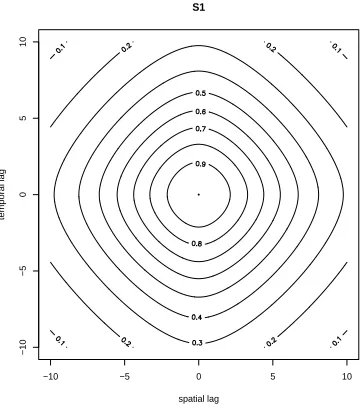
covari-ances except for S1, and the power is close to 1 when nonseparable covaricovari-ances are used. The contour plot for the separable covariance model S1 is shown in Figure 3.1. For small spatial and temporal distance, the shape of S1 is quite similar to a nonseparable covariance, for example the nonseparable covariance model N1 in Figure 3.2. This similarity leads to a large power (Type I error) for the test for separable covariance S1. The contour plots for nonseparable covariance models, N2 and N3, are shown in Figure 3.3 and 3.4. They have similar shapes, but nonseparable covariance N3 has a larger temporal range. By tempo-ral range, we mean the autocorrelation decay by projecting spatial-tempotempo-ral covariance on temporal domain. For the model N3, it has a stronger space-time dependency compared the model N2. Therefore, as shown in Table 3.2, the power of the test for model N3 is larger than N2, but the power of the test for model N2 is still acceptable.

The spatial block bootstrap method might help us to get a finer empirical dis-tribution of the ratio. But the bootstrap blocks should be large enough to preserve the shape of spatial-temporal dependency. This empirical separability test can help us to an-swer the question, which type of covariance, separable or nonseparable, is appropriate for a stationary spatial-temporal process. Moreover, we can get a better idea about if the spatial structure changes over time, and if the temporal structure changes over space.

(43)

spatial lag

temporal lag

−10 −5 0 5 10

−10

−5

0

5

10

S1

Figure 3.1: The contour plot for separable covariance S1.

spatial lag

temporal lag

−10 −5 0 5 10

−10

−5

0

5

10

N1

(44)

spatial lag

temporal lag

−10 −5 0 5 10

−10

−5

0

5

10

N2

Figure 3.3: The contour plot for nonseparable covariance N2.

spatial lag

temporal lag

−10 −5 0 5 10

−10

−5

0

5

10

N3

(45)

3.2 A new class of nonseparable stationary covariance

mod-els

In previous section, we introduced an empirical test for separability. If the result of the test suggests separability, then the existing spatial/temporal covariance models can be employed directly. Otherwise, we need spatial-temporal models to take into account the nonseparability. Nonseparable spatial-temporal models have been proposed by 5), 11), and 31). We introduce a new class of nonseparable stationary covariance structures, and they are used to construct new nonseparable nonstationary models later.

The stationary spatial-temporal process {Z(x, t) : x ∈ D ⊂ Rd, t ∈ T ⊂ R}

can be represented in the spectral domain, instead of space-time domain, which is always interpreted as the superposition of sine and cosine waves of different frequencies (ω, τ), where ω is d-dimensional spatial frequency and τ is temporal frequency. If Z(x, t) is a stationary random field with spatial-temporal covarianceC(x, t), then we can represent the process in the form of the following Fourier-Stieltjes integral (see 36) for example):

Z(x, t) =

Z

Rd

Z

Rexp(iω

T_x₊_{iτ t}₎_dY₍_ω_{, τ}₎_. _(3.4) where Y is a random function that has uncorrelated increments with complex symmetry except for the constraint,dY(ω, τ) =dYc(−ω,−τ), needed to ensureZ(x, t) is real-valued.

Yc denotes the conjugate of Y. Using the spectral representation of Z and proceeding formally,

C(x, t) =

Z

Rd

Z

Rexp(iω

T_x₊_{iτ t}₎_F₍_d_ω_{, dτ}₎_, _(3.5) where the function F is a positive finite measure and is called the spectral measure or spectrum for Z. The spectral measure F is the mean square value of the process Y,

E{|Y(ω, τ)|2}=F(ω, τ).

(46)

definite, since for all finiten, all s₁,· · ·,sn∈Rd×R, and real c1,· · ·, cn, n

X

j,k=1

cjckC(sj −sk) = n

X

j,k=1

cjck

Z

Rd+1exp{iψ

T_(sj₋_s

k)}F(dψ) = Z Rd+1 ¯¯ ¯¯ ¯¯ n X j=1

cjexp(iψTsj)

¯¯ ¯¯ ¯¯ 2

F(dψ)

≥ 0,

wheres= (x, t) and ψ= (ω, τ) are used to simplify the notation.

Theorem 3.2.1 (Bochner’s Theorem). A complex-valued function K onRd_is the autocovariance function for a weakly stationary mean square continuous complex-valued random field onRd if and only if it can be represented as

K(x) =

Z

Rd

exp{iωTx}F(dω),

whereF is a positive finite measure.

Bochner’s theorem gives the relationship between the covariance and the spec-trum for a stationary process. If F has a density with respect to Lebesgue measure, it is the spectral density, f, which is the Fourier transform of the spatial-temporal covariance function:

f(ω, τ) = 1 (2π)d+1

Z

Rd

Z

Rexp(−iω

T_x₋_{iτ t}₎_C_(x_{, t}₎_d_x_dt, _(3.6) and the corresponding covariance function is given by

C(x, t) =

Z

Rd

Z

Rexp(iω

T_x₊_{iτ t}₎_f₍_ω_{, τ}₎_d_ω_dτ. _(3.7) For example, the Mat´etrn spatial spectral density is given by

f(ω) =γ(α2+|ω|2)−ν−d/2,

and its corresponding Mat´ern spatial covariance function is

C(x) = π

d/2_γ 2ν−1_Γ(_ν₊d

2)α2ν

(α|x|)νKν(α|x|),

(47)

When f(ω, τ) =f(1)(ω)f(2)(τ), we obtain cov{Z(x₁, t₁), Z(x₂, t₂)} = C(x₁−x₂, t₁−t₂)

=

Z

Rd

exp{iωT(x₁−x₂)}f(1)(ω)(f(1)(ω))cdω ×

Z

R1exp{iτ(t1−t2)}f

(2)₍_τ₎₍_f(2)₍_τ₎₎c_dτ = C(1)(x₁−x₂)C(2)(t₁−t₂),

which means the corresponding spatial-temporal covariance is separable.

We propose the following spatial-temporal spectral density, that has a separable model as a particular case,

f(ω, τ) =γ(α2β2+β2|ω|2+α2τ2+²|ω|2τ2)−ν, (3.8) whereγ,αandβare positive,ν > d+1₂ and²∈[0,1]. The function in (3.8) is a valid spectral density. First, f(ω, τ)>0 everywhere. Second,f(ω, τ)≤γ(α2β2+β2|ω|2+α2τ2)−ν, and

Z

Rd

Z

Rexp(iω

T_x₊_{iτ t}₎_γ₍_α2_β2₊_β2_|_ω_|2₊_α2_τ2₎−ν_d_ω_dτ

= π

d+1 2 γ

2ν−d+12 −1Γ(ν)α2ν−d_β2ν−1

Ã α

r

(β

αt)2+|x|2

!ν−d+1₂

×

K_ν₋d+1 2

Ã α

r

(β

αt)2+|x|2 !

, (3.9)

Therefore, R_Rd

R

Rexp(iωTx+iτ t)f(ω, τ)dωdτ exists.

When ²= 1, the equation (3.8) can be written as

f(ω, τ) = γ(α2β2+β2|ω|2+α2τ2+|ω|2τ2)−ν = γ(α2+|ω|2)−ν(β2+τ2)−ν.

(48)

spatial lag

temporal lag

−4 −2 0 2 4

−4

−2

0

2

4

epsilon=1

Figure 3.5: The contour plot for a separable spatial-temporal covariance.

When ²= 0,

f(ω, τ) =γ(α2β2+β2|ω|2+α2τ2)−ν. (3.10) The function in (3.10) is an extension of the traditional Mat´ern spectral density. It treats time as an additional component of space, but it does have a different rate of decay. In the spectral density (3.10), the parameter α−1 explains the rate of decay of the spatial correlation. For the temporal correlation, the rate of decay is explained by the parameter

β−1. γ is a scale parameter. The parameter ν measures the degree of smoothness of the processZ. The higher value of ν, the smoother the process Z will be. The corresponding spatial-temporal covariance is give by (3.9), which is a Mat´ern type covariance. Following the parameterization suggested by 16), we have

C(x, t) = σ

2

2ν−1_Γ(_ν₎

µ

k(x, ρt)k

r ¶

Kν

µ

k(x, ρt)k

r ¶

Bayesian Hierarchical Spatial-Temporal Models for Wind Prediction

Contents

List of Figures

List of Tables

Chapter 1

Introduction

1.1

Motivation

1.2

Description of data

1.3

Objectives

Chapter 2

Spatial-Temporal Processes

2.1

Introduction of spatial-temporal processes

2.2

Recent approaches to spatial-temporal processes

x

o.

o

o

o

o

o

o

o

o

o

o

o

o

o

o

o

o

o

o

o

oo

o

o

o

o

2.3

Summary

Chapter 3

Nonseparable and nonstationary

spatial-temporal models

3.1

An empirical test for separability

3.2

A new class of nonseparable stationary covariance

mod-els