A Deterministic Word Dependency Analyzer
Enhanced With Preference Learning
Hideki Isozaki and Hideto Kazawa and Tsutomu HiraoNTT Communication Science Laboratories NTT Corporation
2-4 Hikaridai, Seikacho, Sourakugun, Kyoto, 619-0237 Japan {isozaki,kazawa,hirao}@cslab.kecl.ntt.co.jp
Abstract
Word dependency is important in parsing tech-nology. Some applications such as Informa-tion ExtracInforma-tion from biological documents ben-efit from word dependency analysis even with-out phrase labels. Therefore, we expect an ac-curate dependency analyzer trainable without using phrase labels is useful. Although such an English word dependency analyzer was pro-posed by Yamada and Matsumoto, its accu-racy is lower than state-of-the-art phrase struc-ture parsers because of the lack of top-down in-formation given by phrase labels. This paper shows that the dependency analyzer can be im-proved by introducing a Root-Node Finder and a Prepositional-Phrase Attachment Resolver. Experimental results show that these modules based on Preference Learning give better scores than Collins’ Model 3 parser for these subprob-lems. We expect this method is also applicable to phrase structure parsers.
1 Introduction
1.1 Dependency Analysis
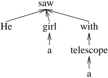
Word dependency is important in parsing technol-ogy. Figure 1 shows a word dependency tree. Eis-ner (1996) proposed probabilistic models of depen-dency parsing. Collins (1999) used dependency analysis for phrase structure parsing. It is also stud-ied by other researchers (Sleator and Temperley, 1991; Hockenmaier and Steedman, 2002). How-ever, statistical dependency analysis of English sen-tences without phrase labels is not studied very much while phrase structure parsing is intensively studied. Recent studies show that Information Ex-traction (IE) and Question Answering (QA) benefit from word dependency analysis without phrase la-bels. (Suzuki et al., 2003; Sudo et al., 2003)
Recently, Yamada and Matsumoto (2003) pro-posed a trainable English word dependency ana-lyzer based on Support Vector Machines (SVM). They did not use phrase labels by considering an-notation of documents in expert domains. SVM (Vapnik, 1995) has shown good performance in
dif-He
a girl
a telescope
with saw
He saw a girl with a telescope.
Figure 1: A word dependency tree
ferent tasks of Natural Language Processing (Kudo and Matsumoto, 2001; Isozaki and Kazawa, 2002). Most machine learning methods do not work well when the number of given features (dimensionality) is large, but SVM is relatively robust. In Natural Language Processing, we use tens of thousands of words as features. Therefore, SVM often gives good performance.
However, the accuracy of Yamada’s analyzer is lower than state-of-the-art phrase structure parsers such as Charniak’s Maximum-Entropy-Inspired Parser (MEIP) (Charniak, 2000) and Collins’ Model 3 parser. One reason is the lack of top-down infor-mation that is available in phrase structure parsers.
In this paper, we show that the accuracy of the word dependency parser can be improved by adding a base-NP chunker, a Root-Node Finder, and a Prepositional Phrase (PP) Attachment Resolver. We introduce the base-NP chunker because base NPs are important components of a sentence and can be easily annotated. Since most words are contained in a base NP or are adjacent to a base NP, we ex-pect that the introduction of base NPs will improve accuracy.
Root Accuracy (RA) =
#correct root nodes / #sentences (= 2,416)
We think that the root node is also useful for depen-dency analysis because it gives global information to each word in the sentence.
Root node finding can be solved by various ma-chine learning methods. If we use classifiers, how-ever, two or more words in a sentence can be classi-fied as root nodes, and sometimes none of the words in a sentence is classified as a root node. Practically, this problem is solved by getting a kind of confi-dence measure from the classifier. As for SVM,
f(x)defined below is used as a confidence measure. However,f(x)is not necessarily a good confidence measure.
Therefore, we use Preference Learning proposed by Herbrich et al. (1998) and extended by Joachims (2002). In this framework, a learning system is trained with samples such as “A is preferable to B” and “C is preferable to D.” Then, the system generalizes the preference relation, and determines whether “X is preferable to Y” for unseen X and Y. This framework seems better than SVM to select best things.
On the other hand, it is well known that attach-ment ambiguity of PP is a major problem in parsing. Therefore, we introduce a PP-Attachment Resolver. The next sentence has two interpretations.
He saw a girl with a telescope.
1) The preposition ‘with’ modifies ‘saw.’ That is, he has the telescope. 2) ‘With’ modifies ‘girl.’ That is, she has the telescope.
Suppose 1) is the correct interpretation. Then, “withmodifiessaw” is preferred to “with mod-ifies girl.” Therefore, we can use Preference Learning again.
Theoretically, it is possible to build a new De-pendency Analyzer by fully exploiting Preference Learning, but we do not because its training takes too long.
1.2 SVM and Preference Learning
Preference Learning is a simple modification of SVM. Each training example for SVM is a pair (yi,xi), where xi is a vector, yi = +1means that xiis a positive example, andyi =−1means that xi is a negative example. SVM classifies a given test vector x by using a decision function
f(x) =wf ·φ(x) +b= ` X
i
yiαiK(x,xi) +b,
where{αi}andbare constants and`is the number of training examples. K(xi,xj) = φ(xi)·φ(xj)is a predefined kernel function. φ(x)is a function that maps a vector x into a higher dimensional space.
Training of SVM corresponds to the follow-ing quadratic maximization (Cristianini and Shawe-Taylor, 2000)
W(α) = ` X
i=1
αi− 1 2
` X
i,j=1
αiαjyiyjK(xi,xj),
where0≤αi ≤C andPi`=1αiyi = 0. Cis a soft margin parameter that penalizes misclassification.
On the other hand, each training example for Preference Learning is given by a triplet (yi,xi.1,xi.2), where xi.1 and xi.2 are vectors. We use xi.∗ to represent the pair (xi.1,xi.2). yi = +1 means that xi.1 is preferable to xi.2. We can regard their difference φ(xi.1) −φ(xi.2) as a positive ex-ample andφ(xi.2)−φ(xi.1)as a negative example. Symmetrically,yi = −1 means that xi.2 is prefer-able to xi.1.
Preference of a vector x is given by
g(x) =wg·φ(x) = ` X
i
yiαi(K(xi.1,x)−K(xi.2,x)).
Ifg(x) > g(x0)holds, x is preferable to x0. Since
Preference Learning uses the difference φ(xi.1)−
φ(xi.2) instead of SVM’s φ(xi), it corresponds to the following maximization.
W(α) = ` X
i=1
αi− 1 2
` X
i,j=1
αiαjyiyjK(xi.∗,xj.∗)
where 0 ≤ αi ≤ C and K(xi.∗,xj.∗) = K(xi.1,xj.1) − K(xi.1,xj.2) − K(xi.2,xj.1) +
K(xi.2,xj.2). The above linear constraint
P`
i=1αiyi = 0 for SVM is not applied to Preference Learning because SVM requires this constraint for the optimalb, but there is nobing(x). Although SVMlight (Joachims, 1999) provides an implementation of Preference Learning, we use our own implementation because the current SVMlight implementation does not support non-linear kernels and our implementation is more efficient.
Herbrich’s Support Vector Ordinal Regression (Herbrich et al., 2000) is based on Preference Learn-ing, but it solves an ordered multiclass problem. Preference Learning does not assume any classes.
2 Methodology
Dependency Analyzer• PP-Attachment Resolver◦
Root-Node Finder◦
Base NP Chunker•
(POS Tagger)
•= SVM,◦= Preference Learning
Figure 2: Module layers in the system
That is, we use Penn Treebank’s Wall Street Journal data (Marcus et al., 1993). Sections 02 through 21 are used as training data (about 40,000 sentences) and section 23 is used as test data (2,416 sentences). We converted them to word dependency data by us-ing Collins’ head rules (Collins, 1999).
The proposed method uses the following proce-dures.
• A base NP chunker: We implemented an SVM-based base NP chunker, which is a sim-plified version of Kudo’s method (Kudo and Matsumoto, 2001). We use the ‘one vs. all others’ backward parsing method based on an ‘IOB2’ chunking scheme. By the chunking, each word is tagged as
– B: Beginning of a base NP, – I: Other elements of a base NP.
– O: Otherwise.
Please see Kudo’s paper for more details.
• A Root-Node Finder (RNF): We will describe this later.
• A Dependency Analyzer: It works just like Ya-mada’s Dependency Analyzer.
• A PP-Attatchment Resolver (PPAR): This re-solver improves the dependency accuracy of prepositions whose part-of-speech tags are IN or TO.
The above procedures require a part-of-speech tagger. Here, we extract part-of-speech tags from the Collins parser’s output (Collins, 1997) for sec-tion 23 instead of reinventing a tagger. According to the document, it is the output of Ratnaparkhi’s tagger (Ratnaparkhi, 1996). Figure 2 shows the ar-chitecture of the system. PPAR’s output is used to rewrite the output of the Dependency Analyzer.
2.1 Finding root nodes
When we use SVM, we regard root-node finding as a classification task: Root nodes are positive exam-ples and other words are negative examexam-ples.
For this classification, each word wi in a tagged sentenceT = (w1/p1, . . . , wi/pi, . . . , wN/pN) is characterized by a set of features. Since the given POS tags are sometimes too specific, we introduce a rough part-of-speechqidefined as follows.
• q = N if p = NN, NNP, NNS, NNPS, PRP, PRP$, POS.
• q = V if p = VBD, VB, VBZ, VBP, VBN.
• q = J if p= JJ, JJR, JJS.
Then, each word is characterized by the following features, and is encoded by a set of boolean vari-ables.
• The word itself wi, its POS tags pi and
qi, and its base NP tag bi = B, I, O. We introduce boolean variables such as current word is John and cur-rent rough POS is J for each of these features.
• Previous word wi−1 and its tags, pi−1, qi−1, andbi−1.
• Next word wi+1 and its tags, pi+1, qi+1, and
bi+1.
• The set of left words {w0, . . . , wi−1}, and their tags,{p0, . . . , pi−1},{q0, . . . , qi−1}, and
{b0, . . . , bi−1}. We use boolean variables such asone of the left words is Mary.
• The set of right words {wi+1, . . . , wN}, and their POS tags, {pi+1, . . . , pN} and
{qi+1, . . . , qN}.
• Whether the word is the first word or not.
We also add the following boolean features to get more contextual information.
• Existence of verbs or auxiliary verbs (MD) in the sentence.
• The number of words between wi and the nearest left comma. We use boolean variables such as near-est left comma is two words away.
• The number of words betweenwiand the near-est right comma.
{(yi,xi.1,xi.2)}, whereyi is always+1, xi.1 corre-sponds to the root node, and xi.2 corresponds to a non-root word in the same sentence. Such a triplet means that xi.1is preferable to xi.2as a root node. 2.2 Dependency analysis
Our Dependency Analyzer is similar to Ya-mada’s analyzer (Yamada and Matsumoto, 2003). While scanning a tagged sentence
T = (w1/p1, . . . , wn/pn) backward from the end of the sentence, each wordwi is classified into three categories: Left, Right, and Shift.1
• Right: Right means that wi directly modifies the right word wi+1 and that no word in T modifies wi. If wi is classified as Right, the analyzer removes wi fromT and wi is regis-tered as a left child ofwi+1.
• Left: Left means thatwi directly modifies the left wordwi−1 and that no word inT modifies
wi. Ifwi is classified as Left, the analyzer re-moveswifromTandwiis registered as a right child ofwi−1.
• Shift: Shift means that wi is not next to its modificand or is modified by another word in
T. If wi is classified as Shift, the analyzer does nothing forwiand moves to the left word
wi−1.
This process is repeated until T is reduced to a single word (= root node). Since this is a three-class problem, we use ‘one vs. rest’ method. First, we train an SVM classifier for each class. Then, for each word inT, we compare their values: fLeft(x),
fRight(x), and fShift(x). If fLeft(x) is the largest, the word is classified as Left.
However, Yamada’s algorithm stops when all words inT are classified as Shift, even whenT has two or more words. In such cases, the analyzer can-not generate complete dependency trees.
Here, we resolve this problem by reclassifying a word inT as Left or Right. This word is selected in terms of the differences between SVM outputs:
• ∆Left(x) =fShift(x)−fLeft(x),
• ∆Right(x) =fShift(x)−fRight(x).
These values are non-negative because fShift(x) was selected. For instance,∆Left(x)'0means that
fLeft(x) is almost equal to fShift(x). If ∆Left(xk) gives the smallest value of these differences, the word corresponding to xkis reclassified as Left. If
1Yamada used a two-word window, but we use a one-word
window for simplicity.
∆Right(xk) gives the smallest value, the word cor-responding to xkis reclassified as Right. Then, we can resume the analysis.
We use the following basic features for each word in a sentence.
• The word itselfwiand its tagspi,qi, andbi,
• Whetherwiis on the left of the root node or on the right (or at the root node). The root node is determined by the Root-Node Finder.
• Whetherwi is inside a quotation.
• Whetherwi is inside a pair of parentheses.
• wi’s left children {wi1, . . . , wik}, which were removed by the Dependency Analyzer beforehand because they were classified as ‘Right.’ We use boolean variables such as one of the left child is Mary. Symmetrically, wi’s right children
{wi1, . . . , wik}are also used.
However, the above features cover only near-sighted information. If wi is next to a very long base NP or a sequence of base NPs,wi cannot get information beyond the NPs. Therefore, we add the following features.
• Li, Ri: Li is available when wi immediately follows a base NP sequence. Liis the word be-fore the sequence. That is, the sentence looks like:
. . .Liha base NPiwi. . .
Riis defined symmetrically.
The following features of neigbors are also used aswi’s features.
• Left wordswi−3, . . . , wi−1and their basic fea-tures.
• Right words wi+1, . . . , wi+3 and their basic features.
• The analyzer’s outputs (Left/Right/Shift) for
wi+1, . . . , wi+3. (This analyzer runs backward from the end ofT.)
2.3 PP attachment
Since we do not have phrase labels, we use all prepositions (except root nodes) as training data. We use the following features for resolving PP at-tachment.
• The preposition itself:wi.
• Candidate modificandwjand its POS tag.
• Left words(wi−2, wi−1)and their POS tags.
• Right words(wi+1, wi+2)and their POS tags.
• Previous preposition.
• Ending word of the following base NP and its POS tag (if any).
• i−j, i.e., Number of the words between wi andwj.
• Number of commas betweenwiandwj.
• Number of verbs betweenwiandwj.
• Number of prepositions betweenwiandwj.
• Number of base NPs betweenwiandwj.
• Number of conjunctions (CCs) betweenwiand
wj.
• Difference of quotation depths betweenwiand
wj. Ifwi is not inside of a quotation, its quo-tation depth is zero. Ifwj is in a quotation, its quotation depth is one. Hence, their difference is one.
• Difference of parenthesis depths between wi andwj.
For each preposition, we make the set of triplets
{(yi,xi,1,xi,2)}, whereyi is always+1, xi,1 corre-sponds to the correct word that is modified by the preposition, and xi,2 corresponds to other words in the sentence.
3 Results
3.1 Root-Node Finder
For the Root-Node Finder, we used a quadratic ker-nelK(xi,xj) = (xi·xj+ 1)2 because it was better than the linear kernel in preliminary experiments. When we used the ‘correct’ POS tags given in the Penn Treebank, and the ‘correct’ base NP tags given by a tool provided by CoNLL 2000 shared task2, RNF’s accuracy was 96.5% for section 23. When we used Collins’ POS tags and base NP tags based on the POS tags, the accuracy slightly degraded to 95.7%. According to Yamada’s paper (Yamada and
2
http://cnts.uia.ac.be/conll200/chunking/
Matsumoto, 2003), this root accuracy is better than Charniak’s MEIP and Collins’ Model 3 parser.
We also conducted an experiment to judge the ef-fectiveness of the base NP chunker. Here, we used only the first 10,000 sentences (about 1/4) of the training data. When we used all features described above and the POS tags given in Penn Treebank, the root accuracy was 95.4%. When we removed the base NP information (bi, Li, Ri), it dropped to 94.9%. Therefore, the base NP information im-proves RNF’s performance.
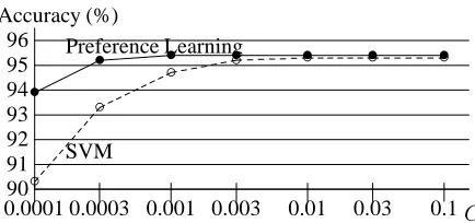
Figure 3 compares SVM and Preference Learn-ing in terms of the root accuracy. We used the first 10,000 sentences for training again. Accord-ing to this graph, Preference LearnAccord-ing is better than SVM, but the difference is small. (They are bet-ter than Maximum Entropy Modeling3 that yielded RA=91.5% for the same data.) Cdoes not affect the scores very much unlessCis too small. In this ex-periment, we used Penn’s ‘correct’ POS tags. When we used Collins’ POS tags, the scores dropped by about one point.
3.2 Dependency Analyzer and PPAR
As for the dependency learning, we used the same quadratic kernel again because the quadratic kernel gives the best results according to Yamada’s experi-ments. The soft margin parameterCis 1 following Yamada’s experiment. We conducted an experiment to judge the effectiveness of the Root-Node Finder. We follow Yamada’s definition of accuracy that ex-cludes punctuation marks.
Dependency Accuracy (DA) =
#correct parents / #words (= 49,892) Complete Rate (CR) =
#completely parsed sentences / #sentences
According to Table 1, DA is only slightly improved, but CR is more improved.
3
http://www2.crl.go.jp/jt/a132/members/mutiyama/ software.html
SVM
Preference Learning Accuracy (%)
C 0.1 0.03 0.01 0.003 0.001 0.0003 0.000190
91 92 93 94 95 96
◦ ◦ ◦ ◦ ◦ ◦
◦
• • • • • • •
DA RA CR without RNF 89.4% 91.9% 34.7% with RNF 89.6% 95.7% 35.7%
The
Dependency Analyzer was trained with 10,000 sentences. RNF was trained with all of the training data.
DA: Dependency Accuracy, RA: Root Acc., CR: Complete Rate
Table 1: Effectiveness of the Root-Node Finder
Accuracy (%)
Figure 4: Comparison of SVM and Preference Learning in terms of Dependency Accuracy of prepositions (Trained with 5,000 sentences)
Figure 4 compares SVM and Preference Learning in terms of the Dependency Accuracy of preposi-tions. SVM’s performance is unstable for this task, and Preference Learning outperforms SVM. (We could not get scores of Maximum Entropy Model-ing because of memory shortage.)
Table 2 shows the improvement given by PPAR. Since training of PPAR takes a very long time, we used only the first 35,000 sentences of the train-ing data. We also calculated the Dependency Accu-racy of Collins’ Model 3 parser’s output for section 23. According to this table, PPAR is better than the Model 3 parser.
Now, we use PPAR’s output for each preposition instead of the dependency parser’s output unless the modification makes the dependency tree into a non-tree graph. Table 3 compares the proposed method with other methods in terms of accuracy. This data except ‘Proposed’ was cited from Yamada’s paper.
IN TO average Collins Model 3 84.6% 87.3% 85.1%
Dependency Analyzer 83.4% 86.1% 83.8% PPAR 85.3% 87.7% 85.7%
PPAR was trained with 35,000 sentences. The number of IN words is 5,950 and that of TO is 1,240.
Table 2: PP-Attachment Resolver
DA RA CR
with MEIP 92.1% 95.2% 45.2% phrase info. Collins Model3 91.5% 95.2% 43.3% without Yamada 90.3% 91.6% 38.4% phrase info. Proposed 91.2% 95.7% 40.7%
Table 3: Comparison with related work
According to this table, the proposed method is close to the phrase structure parsers except Com-plete Rate. Without PPAR, DA dropped to 90.9% and CR dropped to 39.7%.
4 Discussion
We used Preference Learning to improve the SVM-based Dependency Analyzer for root-node finding and PP-attachment resolution. Preference Learn-ing gave better scores than Collins’ Model 3 parser for these subproblems. Therefore, we expect that our method is also applicable to phrase structure parsers. It seems that root-node finding is relatively easy and SVM worked well. However, PP attach-ment is more difficult and SVM’s behavior was un-stable whereas Preference Learning was more ro-bust. We want to fully exploit Preference Learn-ing for dependency analysis and parsLearn-ing, but train-ing takes too long. (Empirically, it takes O(`2)or more.) Further study is needed to reduce the compu-tational complexity. (Since we used Isozaki’s meth-ods (Isozaki and Kazawa, 2002), the run-time com-plexity is not a problem.)
Kudo and Matsumoto (2002) proposed an SVM-based Dependency Analyzer for Japanese sen-tences. Japanese word dependency is simpler be-cause no word modifies a left word. Collins and Duffy (2002) improved Collins’ Model 2 parser by reranking possible parse trees. Shen and Joshi (2003) also used the preference kernelK(xi.∗,xj.∗) for reranking. They compare parse trees, but our system compares words.
5 Conclusions
that SVM was unstable for PP attachment resolu-tion whereas Preference Learning was not. We ex-pect this method is also applicable to phrase struc-ture parsers.
References
Eugene Charniak. 2000. A maximum-entropy-inspired parser. In Proceedings of the North American Chapter of the Association for Compu-tational Linguistics, pages 132–139.
Michael Collins and Nigel Duffy. 2002. New rank-ing algorithms for parsrank-ing and taggrank-ing: Kernels over discrete structures, and the voted percep-tron. In Proceedings of the 40th Annual Meeting of the Association for Computational Linguistics (ACL), pages 263–270.
Michael Collins. 1997. Three generative, lexi-calised models for statistical parsing. In Proceed-ings of the Annual Meeting of the Association for Computational Linguistics, pages 16–23.
Michael Collins. 1999. Head-Driven Statistical Models for Natural Language Parsing. Ph.D. thesis, Univ. of Pennsylvania.
Nello Cristianini and John Shawe-Taylor. 2000. An Introduction to Support Vector Machines. Cam-bridge University Press.
Jason M. Eisner. 1996. Three new probabilistic models for dependency parsing: An exploration. In Proceedings of the International Conference on Computational Linguistics, pages 340–345. Ralf Herbrich, Thore Graepel, Peter
Bollmann-Sdorra, and Klaus Obermayer. 1998. Learning preference relations for information retrieval. In Proceedings of ICML-98 Workshop on Text Cate-gorization and Machine Learning, pages 80–84. Ralf Herbrich, Thore Graepel, and Klaus
Ober-mayer, 2000. Large Margin Rank Boundaries for Ordinal Regression, chapter 7, pages 115–132. MIT Press.
Julia Hockenmaier and Mark Steedman. 2002. Generative models for statistical parsing with combinatory categorial grammar. In Proceedings of the 40th Annual Meeting of the Association for Computational Linguistics, pages 335–342. Hideki Isozaki and Hideto Kazawa. 2002. Efficient
support vector classifiers for named entity recog-nition. In Proceedings of COLING-2002, pages 390–396.
Thorsten Joachims. 1999. Making large-scale support vector machine learning practical. In B. Sch¨olkopf, C. J. C. Burges, and A. J. Smola, editors, Advances in Kernel Methods, chapter 16, pages 170–184. MIT Press.
Thorsten Joachims. 2002. Optimizing search en-gines using clickthrough data. In Proceedings of the ACM Conference on Knowledge Discovery and Data Mining.
Taku Kudo and Yuji Matsumoto. 2001. Chunking with support vector machines. In Proceedings of NAACL-2001, pages 192–199.
Taku Kudo and Yuji Matsumoto. 2002. Japanese dependency analysis using cascaded chunking. In Proceedings of CoNLL, pages 63–69.
Mitchell P. Marcus, Beatrice Santorini, and Mary A. Marcinkiewicz. 1993. Building a large annotated corpus of english: the penn treebank. Computa-tional Linguistics, 19(2):313–330.
Adwait Ratnaparkhi. 1996. A maximum entropy part-of-speech tagger. In Proceedings of the Con-ference on Empirical Methods in Natural Lan-guage Processing.
Libin Shen and Aravind K. Joshi. 2003. An SVM based voting algorithm with application to parse reranking. In Proceedings of the Seventh Confer-ence on Natural Language Learning, pages 9–16. Daniel Sleator and Davy Temperley. 1991. Parsing English with a Link grammar. Technical Report CMU-CS-91-196, Carnegie Mellon University. Kiyoshi Sudo, Satoshi Sekine, and Ralph Grishman.
2003. An improved extraction pattern represen-tation model for automatic IE pattern acquisi-tion. In Proceedings of the Annual Meeting of the Association for Cimputational Linguistics, pages 224–231.
Jun Suzuki, Tsutomu Hirao, Yutaka Sasaki, and Eisaku Maeda. 2003. Hierarchical direct acyclic graph kernel: Methods for structured natural lan-guage data. In Proceedings of ACL-2003, pages 32–39.
Vladimir N. Vapnik. 1995. The Nature of Statisti-cal Learning Theory. Springer.