Learning Word Meta Embeddings by Autoencoding

Proceedings of the 27th International Conference on Computational Linguistics, pages 1650–1661 1650

Learning Word Meta-Embeddings by Autoencoding

Cong Bao

Department of Computer Science University of Liverpool sgcbao2@liverpool.ac.uk

Danushka Bollegala

Department of Computer Science University of Liverpool danushka@liverpool.ac.uk

Abstract

Distributed word embeddings have shown superior performances in numerous Natural Language Processing (NLP) tasks. However, their performances vary significantly across different tasks, implying that the word embeddings learnt by those methods capture complementary aspects of lexical semantics. Therefore, we believe that it is important to combine the existing word em-beddings to produce more accurate and completemeta-embeddings of words. We model the meta-embedding learning problem as an autoencoding problem, where we would like to learn a meta-embedding space that can accurately reconstructallsource embeddings simultaneously. Thereby, the meta-embedding space is enforced to capture complementary information in differ-ent source embeddings via a coherdiffer-ent common embedding space. We propose three flavours of autoencoded meta-embeddings motivated by different requirements that must be satisfied by a meta-embedding. Our experimental results on a series of benchmark evaluations show that the proposed autoencoded embeddings outperform the existing state-of-the-art meta-embeddings in multiple tasks.

1 Introduction

Representing the meanings of words is a fundamental task in Natural Language Processing (NLP). A popular approach to represent the meaning of a word is to embedit in some fixed-dimensional vector space (Turney and Pantel, 2010). In contrast to sparse and high-dimensional counting-based distri-butional word representation methods that use co-occurring contexts of a word as its representation, dense and low-dimensional prediction-based distributed word representations (Pennington et al., 2014; Mikolov et al., 2013a; Huang et al., 2012; Collobert and Weston, 2008; Mnih and Hinton, 2009) have obtained impressive performances in numerous NLP tasks such as sentiment classification (Socher et al., 2013), and machine translation (Zou et al., 2013).

Previous works studying the differences in word embedding learning methods (Chen et al., 2013; Yin and Sch¨utze, 2016) have shown that word embeddings learnt using different methods and from differ-ent resources have significant variation in quality and characteristics of the semantics captured. For example, Hill et al. (2014; 2015) showed that the word embeddings trained from monolingual vs. bilin-gual corpora capture different local neighbourhoods. Bansal et al. (2014) showed that an ensemble of different word representations improves the accuracy of dependency parsing, implying the complemen-tarity of the different word embeddings. This suggests the importance ofmeta-embedding– creating a new embedding by combining different existing embeddings. We refer to the input word embeddings to the meta-embedding process as the source embeddings. Yin and Sch¨utze (2016) showed that by meta-embedding five different pre-trained word embeddings, we can overcome the out-of-vocabulary problem, and improve the accuracy of cross-domain part-of-speech (POS) tagging. Encouraged by the above-mentioned prior results, we expect an ensemble containing multiple word embeddings to produce better performances than the constituent individual embeddings in NLP tasks.

Despite the above-mentioned benefits, learning a single meta-embedding from multiple source em-beddings remains a challenging task due to several reasons. First, the algorithms used for learning the source word embeddings often differ significantly and it is non-obvious how to reconcile their differ-ences. Second, the resources used for training source embeddings such as text corpora or knowledge bases are different, resulting in source embeddings that cover different types of information about the words they embed. Third, the resources used to train a particular source embedding might not be pub-licly available for us to train all source embeddings in a consistent manner. For example, the Google news corpus containing 100 billion tokens on which the skip-gram embeddings are trained and released originally by Mikolov et al. (2013b) is not publicly available for us to train other source embedding learning methods on the same resource. Therefore, a meta-embedding learning method must be able to learn meta-embeddings from the given set of source embeddings without assuming the availability of the training resources.

Autoencoders (Kingma and Welling, 2014; Vincent et al., 2008) have gained popularity as a method for learning feature representations from unlabelled data that can then be used for supervised learning tasks. Autoencoders have been successfully applied in various NLP tasks such as domain adaptation (Chen et al., 2012; Ziser and Reichart, 2016), similarity measurement (Li et al., 2015; Amiri et al., 2016), machine translation (P et al., 2014; Li et al., 2013) and sentiment analysis (Socher et al., 2011). Autoencoder attempts to reconstruct an input from a possibly noisy version of the input via a non-linear transformation. The intermediate representation used by the autoencoder captures the essential information about the input such that it can be accurately reconstructed. This setting is closely related to the meta-embedding learning where we must reconstruct the information contained in individual source embeddings using a single meta-embedding. However, unlike typical autoencoder learning where we have a single input, in meta-embedding learning we must reconstruct multiple source embeddings.

We propose three types of autoencoders for the purpose of learning meta-embeddings. The three types consider different levels of integrations among the source embeddings. To the best of our knowledge, autoencoders have not been used for meta-embedding learning in prior work. We compare the proposed autoencoded meta-embeddings (AEME) against previously proposed meta-embedding learning meth-ods and competitive baselines using five benchmark tasks. Our experimental results show that AEME outperforms the current state-of-the-art meta-embeddings in multiple tasks.

2 Related Work

Yin and Sch¨utze (2016) proposed a meta-embedding learning method (1TON) that projects a meta-embedding of a word into the source meta-embeddings using separate projection matrices. The projection matrices are learnt by minimising the sum of squared Euclidean distance between the projected source embeddings and the corresponding original source embeddings for all the words in the vocabulary. They propose an extension (1TON+) to their meta-embedding learning method that first predicts the source word embeddings for out-of-vocabulary words in a particular source embedding, using the known word embeddings. Next, 1TON method is applied to learn the meta-embeddings for the union of the vocabu-laries covered by all of the source embeddings. Experimental results in semantic similarity prediction, word analogy detection, and cross-domain POS tagging tasks show the effectiveness of both 1TON and 1TON+.

Although not learning any meta-embedding, several prior works have shown that incorporating mul-tiple word embeddings learnt using different methods improve performance in various NLP tasks. For example, Tsuboi (2014) showed that by using both word2vec and GloVe embeddings together in a POS tagging task, it is possible to improve the tagging accuracy, if we had used only one of those embeddings. Similarly, Turian et al. (2010) collectively used Brown clusters, CW and HLBL embeddings, to improve the performance of named entity recognition and chucking tasks.

whereas, we consider source embeddings trained using different word embedding learning methods and resources. Although their method could be potentially extended to meta-embed different source embed-dings, the unavailability of their implementation prevented us from exploring this possibility.

Goikoetxea et al. (2016) showed that concatenation of word embeddings learnt separately from a cor-pus and the WordNet to produce superior word embeddings. Moreover, performing Principal Component Analysis (PCA) on the concatenated embeddings slightly improved the performance on word similarity tasks.

Chandar et al. (2015) proposed a correlation neural network that reconstruct an input using two views such that their correlation in a hidden layer os maximised. The setting of this work, using multiple views for reconstructing, is similar to our multiple source embeddings. However, we do not optimise simply for correlation, but require reconstructing the sources from meta-embeddings. Moreover, Chandar et al. (2015) did not consider meta-embedding learning, which is the focus of this paper.

3 Autoencoded Meta-Embeddings

To simplify the disposition of the proposed method, we focus on the problem of learning a single meta-embedding from two given source meta-embeddings. The autoencoding methods we propose in this paper can be easily generalised to more than two source embeddings. Let us denote the two source embeddings by

S1andS2. Moreover, the dimensionalities of two source embeddingsS1andS2are given respectivelyd1 andd2. Note that we do not assumed1 andd2 to be equal. The two word embeddings of a wordw∈ V is given respectively bys1(w)∈Rd1 ands2(w)∈Rd2. Here, the vocabularyVis the intersection set of

two vocabulariesV1andV2of source embeddingsS1 andS2, i.e. V = V1∩ V2. For out of vocabulary words, we can first train a regression model using source embeddings for the common vocabulary as done by Yin and Sch¨utze (2016) and then use it to predict the source embeddings for the words that do not occur in the intersection of the vocabularies.

Next, let us consider two encodersE1andE2, which encode the two source embeddings to a common meta-embedding space M with dimensionality dm for each word w ∈ V. Dimensionalities of the

encoded source embeddings are denoted respectively byd0₁andd0₂. We denote the meta-embedding of a wordw∈ V asm(w) ∈_Rdm_{. Correspondingly, we have two decodersD}

1 andD2, which will decode each wordw ∈ V in the meta-embedding spaceMback to the two original source embeddingsS1 and

S2. Both encoders and decoders can be single or multi-layer neural networks.

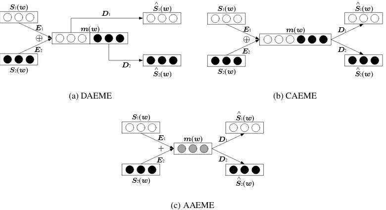
We consider the problem of learningE1, E2, D1 andD2 such that we can learn a meta-embedding m(w)for a wordwconsidering the complementary information from its source embeddingss1(w)and s2(w). We propose three different autoencoding methods for this purpose. The architectures of the three autoencodes are visualised in Figure 1.

3.1 Decoupled Autoencoded Meta-Embedding (DAEME)

In DAEME, the meta-embeddingm(w)is represented as the concatenation of two encoded source em-beddingsE1(s1(w))andE2(s2(w))for each wordw∈ V, as given by (1).

m(w) =E1(s1(w))⊕E2(s2(w)) (1)

Concatenation has been found to be a simple yet effective baseline for creating meta-embeddings from multiple source embeddings. DAEME can be seen as an extension of concatenation that has non-linear neural networks applied on the raw model. Here, each encoder can be seen as independently performing a transformation to the respective source embedding so that it can learn to retain essential information rather than simply concatenate features.

S1(w)

S2(w)

S1(w)

S2(w) ^ ^ E1 E2 D1 D2 m(w)

+

(a) DAEME

S1(w)

S2(w)

S1(w)

S2(w) ^

^

m(w)

E1 E2 D1 D2 + (b) CAEME

S1(w)

S2(w)

S1(w)

S2(w) ^ ^ E1 E2 D1 D2 m(w)

+

(c) AAEME

Figure 1: The architectures of proposed AEMEs. Rectangles represent word vectors, circles represent a single dimension of a word vector, and filled circles represent source of word embeddings. In (c), greyed circles inm(w)indicates mixing of vectors from the two source embeddings.

The reconstructed versions of the two source embeddings are given by (2) and (3).

ˆ

s1(w) =D1(E1(s1(w))) (2)

ˆ

s2(w) =D2(E2(s2(w))) (3)

To encourage encoded embeddings share common information from the two sources, while retaining complementary information, we propose the loss given by (4).

L(E1, E2, D1, D2) =

X

w∈V

λ1||E1(s1(w))−E2(s2(w))||2 (4)

+λ2||ˆs1(w)−s1(w)||2+λ3||ˆs2(w)−s2(w)||2

The first term in the RHS of (4) emphasises the common information to the two source, whereas the second and third terms force the meta-embedding to retain sufficient information to reconstruct the two source embeddings. The coefficientsλ1,λ2, andλ3in (4) can be used to control the effect of the three errors on the overall objective. Later in our experiments, we set these coefficients using validation data. We jointly learnE1, E2, D1 andD2 such that the total reconstruction error given by (4) is minimised. To prevent the weight matrices of the autoencoders degrading to the identity matrixIduring training, we use a non-linear activation function (ReLU in our experiments) in encoders.

3.2 Concatenated Autoencoded Meta-Embedding (CAEME)

Similar to DAEME, the meta-embedding in CAEME is also constructed as the concatenation of two encoded source embeddings as described in (1). However, instead of treating the meta-embedding as two individual components, CAEME reconstructs the source embeddings from thesamemeta-embedding, thereby implicitly using both common and complementary information in the source embeddings. The reconstructed source embeddings for CAEME are given by (5) and (6).

ˆ

s1(w) =D1(m(w)) (5)

ˆ

In CAEME, the dimensionality of the meta-embedding spaceMis identical to that of DAEME, which isdm =d01+d02. The overall objective of CAEME is given by (7). Similar to DAEME, the coefficients

λ1andλ2 can be used to give different emphasis to the reconstruction of the two sources. For example, if we would like to emphasis reconstructingS₂more thanS₁in the meta-embedding process, we can set

λ2> λ1. The coefficients are also tuned experimentally using validation data.

L(E1, E2, D1, D2) =

X

w∈V

λ1||ˆs1(w)−s1(w)||2+λ2||ˆs2(w)−s2(w)||2

(7)

Compared to DAEME, CAEME imposes a tighter integration between the two sources in their meta-embedding. We jointly learnE1, E2, D1 andD2 that minimises the total reconstruction error given by (7).

3.3 Averaged Autoencoded Meta-Embedding (AAEME)

AAEME can be seen as a special case of CAEME, where we compute the meta-embedding by averaging the two encoded sources in (1) instead by their concatenation. A recent work (Coates and Bollegala, 2018) shows that for approximately orthogonal source embedding spaces, averaging performs compa-rably to concatenation, without increasing the dimensionality. However, our AAEME can be seen as a more general version of averaging in the sense that we first transform each source embedding indepen-dently using two encoders before we compute their average. This operation has the benefit that we can transform the sources such that they could be averaged in the same vector space, and also guarantees orthogonality between the encoded vectors. AAEME computes the meta-embedding of a wordwfrom its two source embeddingss1(w)ands2(w)as the`2-normalised1sum of two encoded versions of the source embeddingsE1(s1(w))andE2(s2(w)), given by (8).

m(w) = E1(s1(w)) +E2(s2(w))

||E1(s1(w)) +E2(s2(w))||₂

(8)

Note that unlike CAEME, where the outputs of the two encoders might be of different dimension-alities, in AAEME they should be equal in order to facilitate summation. One could set the output dimensionalities of the two encoders to be different and pad zeros to the shorter output vector. However, we did not find this trick to perform well empirically in our preliminary experiments and do not consider output encodings of different dimensionalities in AAEME. Similar to CAEME, the two source embed-dings are reconstructed from the same meta-embedding using two separate decodersD1andD2as given by (5) and (6). The overall reconstruction error for AAEME is the same as in (7).

4 Experiments

4.1 Source Word Embeddings

We use the following two source embeddings in our experiments:

CBOW: The Continuous Bag-Of-Words (CBOW) embeddings proposed by Mikolov et al. (2013a). The released version we used contains 929,019 word embeddings (phrase embeddings are discarded) with dimensionality of 300, and is trained on Google News corpus (about 100 billion words).

GloVe: The Global Vectors for word representation proposed by Pennington et al. (2014). The released version we used contains 1,917,494 word embeddings with dimensionality of 300 that is trained on Common Crawl dataset.

The intersection of two vocabularies contains 154,076 words for which we create meta-embeddings. We choose CBOW and GloVe as the source embeddings because according to Yin and Sch¨utze (2016), CBOW and GloVe outperform other previously proposed word embeddings such as HLBL (Mnih and Hinton, 2009) and Huang (Huang et al., 2012) in several benchmark tasks such as semantic similarity measurement and word analogy prediction. However, we emphasise that all three proposed methods can be trained with more than two source embeddings.

1_{In our preliminary experiments we found`}

4.2 Training Details

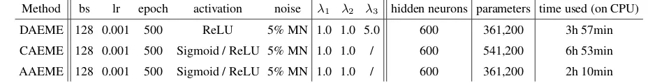
In our experiments, each autoencoder is implemented as a neural network with a single hidden layer. The weights of the encoders and decoders are randomly initialised by sampling from a Gaussian with zero mean and 0.01 standard deviation. We use Adam (Kingma and Ba, 2014) with mini-batches of size 128 for minimising the reconstruction error in each variant of AEME. Masking noises (MN) (Vincent et al., 2010) is applied during training, which will randomly set a fraction of the elements in an input vector to zero. Table 1 summarises hyperparameters, overall trainable parameters, and the time consumed by each method. The optimal hyperparameters were found using the Miller-Charles dataset as a validation dataset. Code implementing AEMEs is publicly available2.

Method bs lr epoch activation noise λ1 λ2 λ3 hidden neurons parameters time used (on CPU)

DAEME 128 0.001 500 ReLU 5% MN 1.0 1.0 5.0 600 361,200 3h 57min

CAEME 128 0.001 500 Sigmoid / ReLU 5% MN 1.0 1.0 / 600 541,200 6h 53min

AAEME 128 0.001 500 Sigmoid / ReLU 5% MN 1.0 1.0 / 600 361,200 2h 10min

Table 1: Training details. bs: batch size. lr: learning rate. Both Sigmoid and ReLU activations per-formed comparably for CAEME and AAEME in our experiments.

4.3 Evaluation Tasks

Following the common practice for evaluating word embeddings, we use the meta-embeddings created by the proposed method in a set of NLP tasks and measure the increase/decrease of the performance of those tasks. If a meta-embedding can improve the performance of an NLP task, then it can be considered as an accurate semantic representation for the words. All meta-embeddings compared in our experiments cover the same subset of words that appear in the benchmark dataset. Therefore, there is no unfair advantage to a particular meta-embedding method due to its coverage of the vocabulary. We use the following five evaluation tasks:

Semantic Similarity: The semantic similarity between two words is measured as the cosine similarity between the corresponding word embeddings. The computed semantic similarity scores are com-pared against human-rated similarity scores using the Spearman correlation coefficient. A high degree of correlation with the human ratings is considered as an indication of the accuracy of the word embeddings. We use the following benchmark datasets for this evaluation: Word Similar-ity 353 dataset (WS, 2023 word pairs) (Finkelstein et al., 2002), Rubenstein-Goodenough dataset (RG, 65 word pairs) (Rubenstein and Goodenough, 1965), Miller-Charles dataset (MC, 30 word pairs) (Miller and Charles, 1998), and theMENdataset (3000 word pairs) (Bruni et al., 2012).

Word Analogy: Word analogy task consists of questions like “a to b is c to what?”. Different methods have been proposed in the literature for finding fourth worddthat completes an analogy. In our experiments we use the CosAdd method, which findsdsuch that the cosine similarity between the vector(b−a+c) anddis maximised. We use the following benchmark datasets for this task: Google dataset (GL) (Mikolov et al., 2013b), MSRdataset (Levy and Goldberg, 2014), SemEval 2012 Task 2 dataset (SE) (Jurgens et al., 2012), and theSAT(Slack, 1980) dataset. The evaluation measure is the ratio of the questions that were answered correctly in each dataset using a particular word embedding.

Relation Classification: The DiffVec dataset (DV) (Vylomova et al., 2016) contains 12,458 triples of the form(r, w1, w2), where the relationrexists between the two wordsw1andw2. DiffVec dataset contains tuples covering 15 different relation types. The task is to predict the relation that exists between two wordsw1 andw2from the 15 relation types in the dataset. The relation classification accuracy is computed as the ratio of the correctly predicted instances to the total instances in the

DiffVec dataset. We represent the relation between two words as the vector offset,w1−w2, between the corresponding word embeddings. Next, we measure cosine similarity between the target test word-pair and word-pairs in the training dataset and use a 1-nearest neighbour classifier to predict the relation for the test word-pair.

Short-text Classification: In the short-text classification task, a text is represented by the centroid of the embeddings of the words contained in that text. All datasets used in the short-text classification tasks contain binary target labels. We train a binary logistic regression classifier using the train part of each dataset and the classification accuracy is measured on the test part of the corresponding dataset. We use the following short-text classification datasets in our experiments: Stanford Sen-timent Treebank (TR) (Socher et al., 2013), Movie Review dataset (MR) (Pang and Lee, 2005), Customer Review dataset (CR) (Hu and Liu, 2004), and Subjectivity dataset (SUBJ) (Pang and Lee, 2004).

Psycholinguistic Score Prediction: Word embeddings can be used as features for predicting psycholin-guistic ratings of a word (Paetzold and Specia, 2016). We use the learnt meta-embeddings in a neu-ral network (containing a single hidden layer of 100 neurones and ReLU as the activation function) to learn a regression model for predicting different psycholinguistic ratings. We use a randomly selected 80% of words from the MRC database3 and the ANEW dataset (Beth Warriner et al., 2013) to train regression models for arousal (AS), valence (VAL), and dominance (DOM). Pearson correlation between the predicted ratings and human ratings is used as the evaluation measure.

4.4 Baselines

We compare the meta-embeddings produced by the proposed methods against the following baselines:

Concatenation (CONC): Concatenation of the source embeddings for a particular word has been found to be an effective method for creating meta-embeddings citeYin:ACL:2016. Despite being simple, meta-embeddings created via concatenation have shown good performance in benchmark tasks such as semantic similarity measurement and word analogy detection. We create meta-embeddings by first `2 normalising the CBOW and GloVe embeddings for a word, and then concatenating the normalised embeddings. The normalisation operation gives an equal importance to the source em-beddings when we measure cosine similarity using the concatenated meta-emem-beddings.

Singular Value Decomposition (SVD): A disadvantage of concatenation as a method for creating meta-embeddings is that it increases the dimensionality of the meta-embedding space. For example, if we concatenated two source embeddings of dimensionalitiesd1andd2, the resultant meta-embedding will have a dimensionality of (d1 + d2). SVD has been used in various tasks in NLP such as latent semantic analysis (Deerwester et al., 1990) and latent relational analysis (Turney, 2005) as a technique to reduce the dimensionality of a feature space. Yin and Sch¨utze (2016) proposed the use of SVD to reduce the dimensionality of the meta-embeddings created from concatenation. Specifically, let N represents the number of words common to the vocabularies of CBOW and GloVe embeddings. We first create anN×(d1+d2)matrixCrepresenting the concatenation meta-embedding of all words inV. Next, we perform SVD decomposition onC = UΣV>, where U andVare unitary matrices andΣis a diagonal matrix containing the singular values ofC. We then select largestksingular values fromΣto construct a diagonal matrixΣk, and the corresponding

left singular vectors fromUto construct a matrixUk. Finally, we obtain ourk-dimensional

meta-embeddings given by the rows ofCk =UkΣk. SVD is guaranteed to produce the best (in the sense

of least square error) rankk approximation of a matrix. In our experiments, we use CBOW and GloVe source embeddings of 300 dimensions (d1 = d2 = 300) and createdk = 300dimensional SVD meta-embeddings.

Averaging (AVG): Coates and Bollegala (2018) proposed averaging the source embeddings for a word as a method for creating meta-embeddings. Source embeddings are often trained independently and their vector spaces as well as dimensionalities are different, which is problematic when computing averages. Although it is possible to pad a source embeddings that have fewer dimensions with zero such that all source embeddings have the equal dimensionality, it is still not mathematically valid to add vectors in different spaces. Surprisingly however, Coates and Bollegala (2018) show that aver-aging performs well in a series of benchmark tasks. Moreover, they prove that if word embeddings can be shown to be approximately orthogonal, then averaging will approximate the same informa-tion as concatenainforma-tion, without increasing the dimensionality. Averaging can be seen as a special case of AAEME. Similar to concatenation, we first perform`2-normalisation on both CBOW and GloVe embeddings prior to averaging them to create meta-embeddings. Since averaging of em-bedding does not increase the dimensionality, the final dimension of averaged meta-emem-bedding in our experiments isdm = 300, the same as the dimensionalities of the CBOW and GloVe source

embeddings.

4.5 Evaluation Results

The evaluation results of different embeddings on different tasks or datasets are summarised in Table 2. In Table 2, rows 1 and 2 show the performance of the source embeddings. Performance of baseline methods are shown in rows 3-5, and rows 8-10 are the results for the proposed method. We also include 1TON and 1TON+ proposed by Yin and Sch¨utze (2016) in rows 6 and 7 as a comparison, which is the current state-of-the-art. To make a fair comparison, we use the publicly available meta-embeddings released by Yin and Sch¨utze (2016) in our evaluation and do not retrain their method.

Model WS RG MC MEN GL MSR SE SAT DV TR MR CR SUBJ AS VAL DOM

sources

1 CBOW 69.1 76.0 82.2 78.2 68.2 76.3 43.4 30.2 88.5 80.3 76.2 79.2 90.6 1.97 0.26 2.70

2 GloVe 75.4 82.9 87.0 81.7 70.7 72.3 41.6 27.0 87.8 80.0 75.9 81.5 90.0 3.66 1.19 0.85

ensemble

3 CONC 76.4 83.0 88.8 82.5 75.5 79.4 43.5 29.7 88.5 80.6 76.5 80.9 90.7 2.29 1.98 0.00

4 SVD 76.8 83.3 86.7 82.6 76.9 79.8 43.2 30.7 89.5 80.3 77.0 80.9 90.1 1.29 2.07 0.64

5 AVG 76.4 83.0 88.8 82.5 75.5 79.4 43.5 29.7 88.5 81.1 76.8 81.2 90.7 3.18 0.11 0.00

6 1TON 76.5 83.2 88.1 82.8 74.6 78.0 42.3 22.5 87.6 80.7 75.6 81.5 88.7 1.24 5.73 2.74

7 1TON+ 76.8 79.4 85.7 81.8 68.1 72.2 40.1 21.7 83.9 79.4 74.2 68.5 87.1 2.28 11.7 8.27

8 DAEME 77.3 83.0 89.1 83.0 75.9∗ 79.4∗ 43.7 39.3∗ 88.6∗ 82.3 76.6 84.2 90.8∗ 6.97∗ 13.3∗ 6.76

9 CAEME 76.4 84.0 89.3 82.3 74.8 78.6 43.9 38.0∗ 88.2∗ 80.5 76.7 78.9 90.3∗ 5.27∗ 12.1 6.41

10 AAEME 76.1 82.7 88.8 83.2 76.9∗ 80.0∗ 43.8 38.0∗ 89.5∗ 81.4 76.8 82.6 90.3∗ 7.03∗ 13.6∗ 7.35

Table 2: Results on the benchmark tasks. Best results are in bold, whereas statistical significance over 1TON is indicated by an asterisk.

From Table 2, we see that the ensemble methods (3-10) outperform the individual source embed-dings (1-2) in most tasks. Among the proposed methods, DAEME performs best in short-text classifica-tion tasks, while CAEME is competitive in semantic similarity measurement tasks. On the other hand, AAEME performs overall well and obtains the best performance in word analogy, relation classification, and psycholinguistic score prediction tasks. We evaluate statistical significance against both 1TON and 1TON+. For the semantic similarity and psycholinguistic score prediction benchmarks we use Fisher transformation to computep < 0.05confidence intervals for Spearman correlation coefficients. In all other datasets, we use Clopper-Pearson binomial exact confidence intervals atp <0.05.

ensure orthogonality between feature vectors, which is the reason to outperform AVG.

Concerning dimensionality, we see that performing SVD on CONC does not reduce the performance of most tasks, and even outperforms other methods in tasks such as GL, DV, and MR. Among the three proposed methods, both DAEME and CAEME have dimensionality of 600, and AAEME has dimen-sionality of 300. Although AAEME has smaller dimendimen-sionality, it performs similarly to DAEME and CAEME and outperforms them in 6 tasks. Considering the smaller dimensionality and the robust per-formance, among the three variants of AEME proposed in the paper, AAEME is the recommended meta-embedding for practical applications.

Prior work on word embedding learning shows that the dimensionality of the embedding can affect the performance of a downstream NLP application that uses the word embeddings as features (Bolle-gala et al., 2015; Bolle(Bolle-gala et al., 2016). In order to directly compare the proposed meta-embedding learning methods against the current state-of-the-art meta-embedding learning methods under the same dimensionality, we reduce the dimensionality of the meta-embeddings created by the proposed methods to 200 dimensions using SVD, which is the dimensionality of the publicly released 1TON and 1TON+ meta-embeddings. Table 3 shows the results for this evaluation.

From Table 3, we see that the proposed AEMEs still perform well in tasks of word analogy, relation classification, and short-text classification. Comparing with the results in Table 2, we see that the re-duction of dimensionality has not significantly affected the performance on those benchmark datasets. On the other hand, there is a slight drop in performance for the semantic similarity and psycholinguis-tic score prediction tasks when the dimensionality is reduced. Nevertheless, the proposed methods still outperforms 1TON and 1TON+ in majority of the tasks, which shows that the nonlinear transformations learnt by autoencoders to be superior to the linear transformations learnt by 1TON and 1TON+.

Model WS RG MC MEN GL MSR SE SAT DV TR MR CR SUBJ AS VAL DOM

ensemble

1 1TON 76.5 83.2 88.1 82.8 74.6 78.0 42.3 22.5 87.6 80.7 75.6 81.5 88.7 1.24 5.73 2.74

2 1TON+ 76.8 79.4 85.7 81.8 68.1 72.2 40.1 21.7 83.9 79.4 74.2 68.5 87.1 2.28 11.7 8.27

3 DAEME 74.0 81.7 83.7 82.4 77.5∗ 79.2∗ 43.1 38.0∗ 89.7∗ 81.5 76.1 82.9 90.7∗ 5.85∗ 8.81 7.13

4 CAEME 73.7 82.9 85.8 82.5 77.5∗ 80.2∗ 43.6 36.9∗ 89.7∗ 80.6 75.9 79.5 89.8 3.85∗ 0.00 3.20

5 AAEME 74.5 82.0 86.1 82.5 77.6∗ 80.8∗ 43.6 35.0∗ 89.7∗ 81.4 76.4 83.2 90.5∗ 4.13 7.63∗ 6.41

Table 3: Results on the benchmark tasks for 200 dimensional meta-embeddings. Best results are in bold, whereas statistical significance over 1TON is indicated by an asterisk.

5 Conclusion

We proposed three autoencoder-based approaches DAEME, CAEME, and AAEME for learning meta-embeddings from multiple pre-trained source meta-embeddings. The experimental results on a series of bench-mark datasets show that AEME outperforms previously proposed meta-embeddings on multiple tasks. We plan to extend the proposed method to create meta-embeddings from multi-lingual word embeddings.

References

Hadi Amiri, Philip Resnik, Jordan Boyd-Graber, and Hal Daum´e III. 2016. Learning text pair similarity with context-sensitive autoencoders. In Proceedings of the 54th Annual Meeting of the Association for Compu-tational Linguistics (Volume 1: Long Papers), pages 1882–1892, Berlin, Germany, August. Association for Computational Linguistics.

Mohit Bansal, Kevin Gimpel, and Karen Livescu. 2014. Tailoring continouos word representations for dependency parsing. InProc. of ACL.

Danushka Bollegala, Takanori Maehara, and Ken ichi Kawarabayashi. 2015. Embedding semantic relationas into word representations. InProc. of IJCAI, pages 1222 – 1228.

Danushka Bollegala, Alsuhaibani Mohammed, Takanori Maehara, and Ken ichi Kawarabayashi. 2016. Joint word representation learning using a corpus and a semantic lexicon. InProc. of AAAI, pages 2690–2696.

Elia Bruni, Gemma Boleda, Marco Baroni, and Nam Khanh Tran. 2012. Distributional semantics in technicolor. InProc. of ACL, pages 136–145.

Sarath Chandar, Mitesh M. Khapra, Hugo Larochelle, and Balaraman Ravindran. 2015. Correlational neural networks. CoRR, abs/1504.07225.

Minmim Chen, Zhixiang (Eddie) Xu, and Kilian Q. Weinberger. 2012. Marginalized denoising autoencoders for domain adaptation. InProc. of ICML.

Yanqing Chen, Bryan Perozzi, Rami Al-Rfou, and Steven Skiena. 2013. The expressive power of word embed-dings. InProc. of ICML Workshop.

Joshua Coates and Danushka Bollegala. 2018. Frustratingly easy meta-embedding – computing meta-embeddings by averaging source word embeddings. InProc. of NAACL-HLT.

Ronan Collobert and Jason Weston. 2008. A unified architecture for natural language processing: Deep neural networks with multitask learning. InProc. of ICML, pages 160 – 167.

Scott Deerwester, Susan T. Dumais, George W. Furnas, Thomas K. Landauer, and Richard Harshman. 1990. Indexing by latent semantic analysis. JOURNAL OF THE AMERICAN SOCIETY FOR INFORMATION SCI-ENCE, 41(6):391–407.

L. Finkelstein, E. Gabrilovich, Y. Matias, E. Rivlin, z. Solan, G. Wolfman, and E. Ruppin. 2002. Placing search in context: The concept revisited. ACM Transactions on Information Systems, 20:116–131.

Josu Goikoetxea, Eneko Agirre, and Aitor Soroa. 2016. Single or multiple? combining word representations independently learned from text and wordnet. InProc. of AAAI, pages 2608–2614.

Felix Hill, Kyunghyun Cho, S´ebastian Jean, Coline Devin, and Yoshua Bengio. 2014. Not all neural embeddings are born equal. InNIPS workshop.

Felix Hill, Kyunghyun Cho, S´ebastian Jean, Coline Devin, and Yoshua Bengio. 2015. Embedding word similarity with neural machine translation. InICLR Workshop.

Minqing Hu and Bing Liu. 2004. Mining and summarizing customer reviews. InProceedings of the Tenth ACM SIGKDD International Conference on Knowledge Discovery and Data Mining, KDD ’04, pages 168–177, New York, NY, USA. ACM.

Eric H. Huang, Richard Socher, Christopher D. Manning, and Andrew Y. Ng. 2012. Improving word representa-tions via global context and multiple word prototypes. InProc. of ACL, pages 873–882.

David A. Jurgens, Saif Mohammad, Peter D. Turney, and Keith J. Holyoak. 2012. Measuring degrees of relational similarity. InProc. of SemEval.

Diederik P. Kingma and Jimmy Ba. 2014. Adam: A method for stochastic optimization.CoRR, abs/1412.6980.

Diederik P. Kingma and Max Welling. 2014. Auto-encoding variational bayes. InProc. ICLR.

Omer Levy and Yoav Goldberg. 2014. Linguistic regularities in sparse and explicit word representations. In

CoNLL.

Peng Li, Yang Liu, and Maosong Sun. 2013. Recursive autoencoders for ITG-based translation. In Proceed-ings of the 2013 Conference on Empirical Methods in Natural Language Processing, pages 567–577, Seattle, Washington, USA, October. Association for Computational Linguistics.

Jiwei Li, Thang Luong, and Dan Jurafsky. 2015. A hierarchical neural autoencoder for paragraphs and docu-ments. InProceedings of the 53rd Annual Meeting of the Association for Computational Linguistics and the 7th International Joint Conference on Natural Language Processing (Volume 1: Long Papers), pages 1106–1115, Beijing, China, July. Association for Computational Linguistics.

Tomas Mikolov, Kai Chen, and Jeffrey Dean. 2013a. Efficient estimation of word representation in vector space. InProc. of ICLR.

Tomas Mikolov, Ilya Sutskever, Kai Chen, Gregory S. Corrado, and Jeffrey Dean. 2013b. Distributed representa-tions of words and phrases and their compositionality. InProc. of NIPS, pages 3111–3119.

G. Miller and W. Charles. 1998. Contextual correlates of semantic similarity. Language and Cognitive Processes, 6(1):1–28.

Andriy Mnih and Geoffrey E. Hinton. 2009. A scalable hierarchical distributed language model. In D. Koller, D. Schuurmans, Y. Bengio, and L. Bottou, editors,Proc. of NIPS, pages 1081–1088.

Sarath Chandar A P, Sanislas Lauly, Hugo Larochelle, Mitesh M. Khapra, Balaraman Ravindran, Vikas C. Raykar, and Amrita Saha. 2014. An autoencoder approach to learning bilingual word representations. InNIPS’14.

Gustavi Henrique Paetzold and Lucia Specia. 2016. Inferring psycholinguistic properties of words. InProc. of NAACL-HLT, pages 435–440.

Bo Pang and Lillian Lee. 2004. A sentimental education: Sentiment analysis using subjectivity. InProceedings of ACL, pages 271–278.

Bo Pang and Lillian Lee. 2005. Seeing stars: Exploiting class relationships for sentiment categorization with respect to rating scales. InProc. of ACL, pages 115–124.

Jeffery Pennington, Richard Socher, and Christopher D. Manning. 2014. Glove: global vectors for word represen-tation. InProc. of EMNLP, pages 1532–1543.

H. Rubenstein and J.B. Goodenough. 1965. Contextual correlates of synonymy. Communications of the ACM, 8:627–633.

Warner Slack. 1980. The scholastic aptitude test: A critical appraisal. Harvard Educational Review, 50(2):154– 175.

Richard Socher, Jeffrey Pennington, Eric H. Huang, Andrew Y. Ng, and Christopher D. Manning. 2011. Semi-supervised recursive autoencoders for predicting sentiment distributions. InProceedings of the 2011 Conference on Empirical Methods in Natural Language Processing, pages 151–161, Edinburgh, Scotland, UK., July. Asso-ciation for Computational Linguistics.

Richard Socher, Alex Perelygin, Jean Wu, Jason Chuang, Christopher D. Manning, Andrew Ng, and Christopher Potts. 2013. Recursive deep models for semantic compositionality over a sentiment treebank. In Proc. of EMNLP, pages 1631–1642.

Yuta Tsuboi. 2014. Neural networks leverage corpus-wide information for part-of-speech tagging. InProc. of EMNLP, pages 938–950.

Joseph Turian, Lev Ratinov, and Yoshua Bengio. 2010. Word representations: A simple and general method for semi-supervised learning. InProc. of ACL, pages 384 – 394.

Peter D. Turney and Patrick Pantel. 2010. From frequency to meaning: Vector space models of semantics.Journal of Aritificial Intelligence Research, 37:141 – 188.

P.D. Turney. 2005. Measuring semantic similarity by latent relational analysis. In Proc. of IJCAI’05, pages 1136–1141.

Pascal Vincent, Hugo Larochelle, Yoshua Bengio, and Pierre-Antonie Manzagol. 2008. Extracting and composing robust features with denoising autoencoders. InICML’08, pages 1096 – 1103.

Pascal Vincent, Hugo Larochelle, Isabelle Lajoie, Yoshua Bengio, and Pierre-Antoine Manzagol. 2010. Stacked denoising autoencoders: Learning useful representations in a deep network with a local denoising criterion. J. Mach. Learn. Res., 11:3371–3408, December.

Ekaterina Vylomova, Laura Rimell, Trevor Cohn, and Timothy Baldwin. 2016. Take and took, gaggle and goose, book and read: Evaluating the utility of vector differences for lexical relational learning. InACL, pages 1671– 1682.

Wenpeng Yin and Hinrich Sch¨utze. 2016. Learning meta-embeddings by using ensembles of embedding sets. In

Yftah Ziser and Roi Reichart. 2016. Neural structural correspondence learning for domain adaptation.arXiv.