Magnetotelluric source effect due to 3D ionospheric current systems using the complex image method for 1D conductivity structures

(1)

Earth Planets Space,51, 933–945, 1999

Magnetotelluric source effect due to 3D ionospheric current systems using

the complex image method for 1D conductivity structures

Ari Viljanen, Risto Pirjola, and Olaf Amm

Finnish Meteorological Institute, Geophysical Research Division, P.O. Box 503, FIN-00101 Helsinki, Finland

(Received December 14, 1998; Revised September 3, 1999; Accepted September 16, 1999)

The complex image method (CIM) is an efficient tool to calculate the electromagnetic field at the earth’s surface produced by 3D ionospheric current systems when the earth has a layered conductivity structure. The calculations are applicable to the estimation of source effects on magnetotelluric data. In this paper CIM is used in connection with some typical high-latitude ionospheric events: a westward travelling surge, a Harang discontinuity, an omega band, and a giant pulsation. The complicated ionospheric current systems are constructed of short horizontal current filaments with vertical currents at both ends. The currents are given numerically on a 50 km×50 km grid covering a region of even 1000 km×2000 km. The investigations indicate that the source distortion very much depends on the event, and may be significant in a wide period range, especially for a resistive earth structure. The source effect seems quite unpredictable. Sometimes the apparent resistivity is larger and sometimes smaller than the plane wave value. At times the source effect is very small even if the ionospheric current is strongly inhomogeneous.

1. Introduction

The usual assumption in magnetotelluric studies of the earth’s conductivity structure is that the primary field pro-duced by ionospheric-magnetospheric currents is laterally uniform, i.e. the plane wave criterion is satisfied. Gener-ally this is the case except for areas near the auroral and equatorial electrojets where the source effect distortion may seriously hamper the interpretation of data (e.g. Mareschal, 1986; Osipovaet al., 1989; Viljanen, 1996; Padilhaet al., 1997). A careful selection of events to be analyzed may de-crease the source distortion, and robust techniques to deal with data contaminated by source effects have also been de-veloped and applied (e.g. Chaveet al., 1987; Egbert and Booker, 1989a,b; Viljanenet al., 1993; Larsenet al., 1996; Garciaet al., 1997). However, the source currents constitute a complicated 3D system which changes from event to event in an unpredictable way.

H¨akkinen and Pirjola (1986) derived exact formulas for the electromagnetic field at the surface of a 1-D, layered earth assuming a 3D ionospheric-magnetospheric current system. However, the expressions are complicated inverse Fourier transforms and thus impractical in any time-critical applica-tions. Pirjola (1992) and Viljanenet al.(1993) demonstrate the use of the 3D model for magnetotelluric source effect investigations.

The calculation of the surface fields is greatly simplified and accelerated if the contribution of a layered earth is repre-sented by an image of the primary ionospheric source. This technique generally leads to a complex image depth, which can be regarded just as a mathematical trick. However, the

Copy right cThe Society of Geomagnetism and Earth, Planetary and Space Sciences (SGEPSS); The Seismological Society of Japan; The Volcanological Society of Japan; The Geodetic Society of Japan; The Japanese Society for Planetary Sciences.

real and imaginary parts also imply the depths of the in-phase and out-of-phase telluric currents (Weidelt, 1972; Szarka and Fischer, 1989). The use of the complex image method (CIM) was suggested by Wait and Spies (1969), and reconsidered by Boteler and Pirjola (1998). Applying the study by Thomson and Weaver (1975), Pirjola and Viljanen (1998) extended the CIM concept to the case of a straight horizontal current of a finite length over a layered earth. Vertical currents at both ends of this current are determined by the condition that the total current is divergence-free.

The assumption of strictly vertical currents is reasonable in the auroral region where the inclination is close to 90 degrees (Amm, 1995). The extension of the image method is based on the fact that vertical currents are equivalent to a horizontal current distribution as concerns the magnetic field and the total horizontal electric field at the earth’s surface.

Any ionospheric current distribution can be superposed of the above-described elementary current filaments lying at specified grid points. So the results by Pirjola and Viljanen (1998) permit the treatment of any current system. CIM is also an excellent tool in studies of geomagnetically induced currents (GIC) in technological systems (Pirjolaet al., 1999), where the knowledge of the electric field is crucial.

In this paper we apply CIM to the calculation of the elec-tromagnetic field at the earth’s surface in several realistic cases: a westward travelling surge (WTS), a Harang discon-tinuity, an omega band, and a giant pulsation. For compar-ison, we also consider a plane wave and a line current of a finite length. This paper is also a preparatory work for analy-ses of the data collected in the Baltic Electromagnetic Array Research (BEAR) project (Korja, 1998).

(2)

934 A. VILJANENet al.: SOURCE EFFECT STUDIES WITH THE COMPLEX IMAGE METHOD

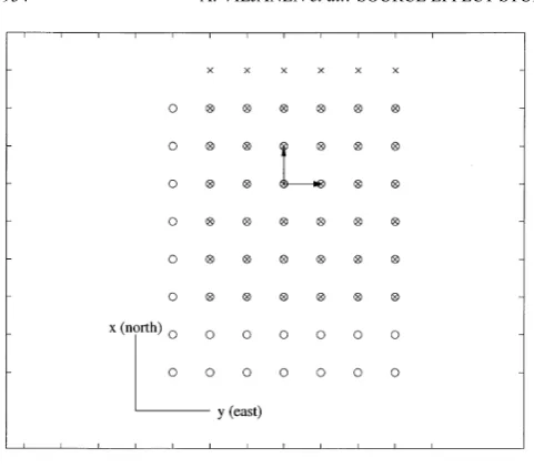
Fig. 1. Synchronized ionospheric (marked with“”) and earth surface (“×”) grids (top view). Two horizontal current elements are shown. Vertical currents start or end at the grid points. In this paper,xpoints to the (geographic) north,yeast,zdownwards, and the earth’s surface is thex yplane.

2. CIM Algorithm

We construct the ionospheric current system of short straight horizontal filaments with vertical currents at both ends. The most practical way is to use northward and east-ward elements set on a rectangular grid. Thefield is cal-culated at the earth’s surface on another grid, which can be defined independently of the ionospheric grid. However, computations become faster if the surface grid is synchro-nized with the ionospheric one as in Fig. 1. The elements are set in such way on the grid that the vertical currents are at the grid points. In this paper the ionospheric and earth grids have the same spacing. Thus, any grid point in the ionosphere can be reached through a multiple shift (measured in the grid spacing) of any earth grid point. The coordinate system is the standard one withxpointing northward,yeastward and

z downward. The earth’s surface is thex y plane, and the ionospheric plane lies atz= −h. Thefield formulas for an eastward elementary current are given in the Appendix.

The amplitude of the current is given as a time series for each element. To be able to use CIM formulas, we apply FFT (fast Fourier transform). For each frequency, the complex image depth is determined by the surface impedance, and the electromagneticfield is obtained from analytical formulas. All current elements are treated in the same way, and the totalfield is the sum of theirfields. The time domainfield is obtained by the inverse FFT.

3. Numerical Results

The ionospheric current models applied here are deter-mined by using ground magnetic data and partly also iono-spheric radar observations (Amm, 1995, 1996). Two differ-ent layered earth models, represdiffer-enting a conductive and a resistive structure, are considered (Table 1). The models are adopted from Viljanen and Pirjola (1994), and a conductive basement starting at the depth of 150 km is added in both. Al-though these models are based on earlier studies in Finland,

Table 1. Conductive and resistive earth models. The cumulative conduc-tance is given at the bottom of each layer.

Conductive model

Depth [km] Resistivity [m] Conductance [1/]

0–3 5000 0.6

Depth [km] Resistivity [m] Conductance [1/]

0–12 30000 0.4

Fig. 2. Absolute value of the complex skin depth. Uniform line: conductive earth model, dashed line: resistive model.

they are only used here as examples of two fairly different cases. The corresponding complex skin depths are shown in Fig. 2.

(3)

A. VILJANENet al.: SOURCE EFFECT STUDIES WITH THE COMPLEX IMAGE METHOD 935

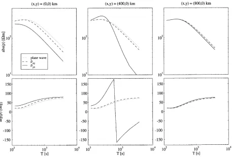
Fig. 3. Absolute values and phases of the apparent resistivitiesρx yandρyxas a function of period atx=0, 400, 800 km (y=0 km) in the case of a line currentflowing above theyaxis at the height of 110 km from(x,y)=(0,−500)km to(x,y)=(0,500)km with vertical currents at the ends. The resistive earth model is used. The plane wave value is plotted as a dotted line.

ρx y(ω,x,y)= −

In the following subsections we briefly outline the iono-spheric current models, and show the apparent resistivity curves. We start with the electrojet model as a basic refer-ence. In all cases the plane wave result is given too.

3.1 Electrojet

Consider a horizontal line currentflowing above theyaxis from(x,y)=(0,−500)km to(x,y)=(0,500)km, with vertical currents at both ends. The horizontal currents are assumed to flow at the height of 110 km throughout this paper. In all examples, the grid spacing is 50 km.

Although the model is an oversimplification, some basic results concerning the apparent resistivity still remain qual-itatively valid in many cases. Figure 3 shows the apparent resistivitiesρx y andρyx at sitesx=0, 400, 800 km (y=0

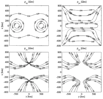
km) for the resistive earth model. All four apparent resistiv-ities are plotted as contour maps in Fig. 4. The conductive model yields qualitatively similar results, but the source dis-tortion is generally smaller.

In the vicinity of the current (x=0),ρyx is smaller than

the plane wave value, then larger (x=400 km), andfinally approaches the plane wave value (x=800 km). Large max-ima are found around aboutx = ±400 km, whereρyxcan be

several times larger than the plane wave value. This is due to the change of sign ofBxnear these points, making the

de-nominator in Eq. (1) very small. The zero points are caused by the opposite signs ofBxdue to the horizontalfilament and the vertical currents. The sign reversal is often seen in ob-served data of long meridional magnetometer chains across the auroral region (e.g. Untiedt and Baumjohann, 1993), and the length of the electrojet considered here has a reasonable value.

The apparent resistivityρx y is quite smooth, butρx x and ρyyare very peculiar even in this simple model. For example, ρx xis exactly zero along theyaxis becauseExvanishes there.

We also checked the accuracy of CIM by considering an infinitely long line current and comparingρyxcalculated with

CIM and from exact integral formulas. For both earth mod-els used here the coindidence is excellent in the period range 100. . .10000 s and at distances 0. . .1000 km from the cur-rent. The largest relative errors in the magnitude are about 10%.

3.2 Westward travelling surge

(4)

Fig. 4. Absolute values of the apparent resistivitiesρx yandρyx(upper panel), andρx xandρyy(lower panel) as a contour map for the electrojet model in Fig. 3. The period is 640 s and the plane wave value of the apparent resistivity is 237m (dotted line).

is constant in the frame which moves with WTS. The time dependence then results from the motion of WTS over the ionospheric grid in Fig. 1. Aroundx=0 kmBxis charater-ized by a negative peak, andBybyfirst a positive and then a smaller negative excursion.

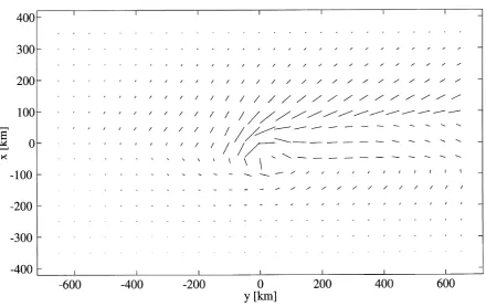
In all models hereafter we have slightly extended the hor-izontal current distribution to avoid unrealistically large ver-tical currents at the boundaries. For clarity, these extensions are not shown in the current model plots. Outside the ex-tended grid all currents are assumed to be zero.

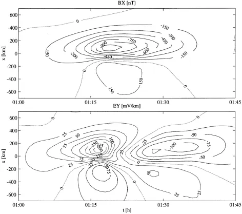
Figure 6 displays thexcomponent of the magneticfield disturbance and the ycomponent of the associated electric

field in the time domain along the profile y = 0 km. For clarity, we have zoomed in the region where the variation is largest. The head of WTS crosses the profile at about 01:20. The currents in Fig. 5 are scaled to yield quite an intense variation at the earth’s surface.

We have smoothed the apparent resistivity curves, because otherwize they are very spiky due to very small values of the electric or magneticfield at some sites (the plane wave curves are not modified). The absolute value at a given period

T is computed byfirst taking the average of|E|2 and|B|2

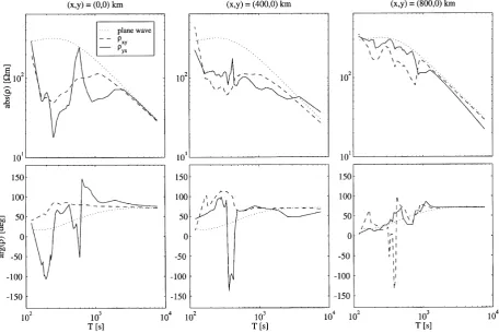
in the period range(T −T,T +T), and then applying Eq. (1). T used here is half of the shortest period available. Figures 7 and 8 show the apparent resistivitiesρx yandρyxat

sitesx=0, 400, 800 km on the profiley=0 km, assuming the conductive and resistive earth models, respectively.

Although the resistivity curves are here and there quite intricate, their basic behaviour is in many cases the same as that of the electrojet: near the current centre the values are smaller, then at long periods larger, and at large distances equal to the plane wave result (cf.ρyxin Fig. 4). The

compli-cated results are expected because even the simple electrojet model produces spatially strongly varying resistivities. In the WTS model thefield at one point is remarkably affected by some tens of nearby current elements, which may have opposite signs and very different amplitudes.

(5)

Fig. 5. Horizontal current distribution associated with the westward travelling surge (WTS). This is the snapshot of the instant when the head of WTS at (x,y)=(0,0)is above the origin of the earth surface grid.

3.3 Harang Discontinuity

A typical local evening ionospheric current system con-sists of the boundary between an eastward and a westward electrojet which are separated by an upward current distri-bution (Fig. 9). We assume that the whole system moves westwards with a velocity of 1 km/s.

The sounding curves are presented in Figs. 10 and 11. Except for some single spikes, the apparent resistivities are nearly identical to the plane wave ones, when the conduc-tive model is considered. Deviations in the resisconduc-tive model are clearly not (only) due to such spikes, but have a more systematic behaviour decreasing the apparent resistivities.

3.4 Omega band

An omega band is an auroral form which resembles the Greek letter (Fig. 12). The associated current system moves eastwards with a typical velocity of 1 km/s. In the time domain a characteristic feature is a positive peak inBy

when the current system moves over an observation point. The sounding curves are presented in Figs. 13 and 14. Their characteristics are comparable to the Harang disconti-nuity case: deviations from the plane wave results are smaller for the conductive earth model than for the resistive one.

3.5 Giant pulsation

A giant pulsation is observed as a nearly sinusoidal time variation of the electromagneticfield. The model used here is based on observations by Glassmeier (1980). The iono-spheric current system consists of a horizontal vortex having vertical currents at its centre and opposite vertical currents at both sides (Fig. 15). In this case the system is moving westwards with about the Earth’s rotation velocity, and each of the elementary currentfilaments has an approximately si-nusoidal time dependence (period 100 s).

Although the ionospheric current is spatially strongly in-homogeneous, the apparent resistivity is nearly equal to that of the plane wave. However, a denser plot ofρyx along the

profiley=0 km would reveal some single spikes. In Fig. 16 we only show the resistive case, because for the conductive model the sounding curves of ρx y andρyx are practically

identical to the plane wave ones. Although the source ef-fect happens to be small along the selected y profile, it is somewhat more severe at some other profiles. In any case, the apparent resistivity is clearly less distorted than in other models.

4. Conclusions

(6)

Fig. 6. Bx(x,t)andEy(x,t)along the profiley=0 km for a WTS moving 1 km/s westwards. The conducitive earth model is used.

al., 1993) or in real data (e.g. Garciaet al., 1997).

There are no large differences in the size of distortion be-tween the two apparent resistivities (ρx yandρyx). However,

at long periodsρx y is generally a little closer to the plane

wave value thanρyx. This is evidently due to the fact that

in most models the ionospheric current system moves in the east-west direction and thus may produce smoother(Ex,By)

than(Bx,Ey). Anyhow, the source effect cannot be directly

estimated from the structure of the ionospheric current. For example, due to a giant pulsation the surfacefield is laterally strongly inhomogeneous, but the apparent resisitivities are nearly identical to the plane wave values.

Our examples concern single events, especially selected to be caused by very inhomogeneous sources. This may give too a pessimistic impression of the source effect. In practical magnetotelluric analysis, long time series and appropriate ro-bust methods are used, so the effect of single peculiar events may well be removed, and naturally there is no reason to consciously select disturbed samples.

Concerning the future work, an important question is whether the small scale variations in the earth’s conductivity affect the electricfield more than the inhomogeneous source

field. It may even turn out that, after all, the local geology is much more dominating than any complicated sourcefield, at least at small periods.

(7)

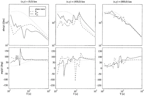
Fig. 7. Absolute values and phases of the apparent resistivitiesρx yandρyxas functions of period atx =0, 400, 800 km (y=0 km) in the case of the WTS model in Fig. 5. The conductive earth model is used. The plane wave value is plotted as a dotted line.

(8)

Fig. 9. Snapshot of the horizontal current system of the Harang discontinuity. Along the boundary between the eastward and westward electrojets there is a sharply concentrated upward current sheet approximately along the diagonal from the upper left corner to the lower right corner.

(9)

Fig. 11. As Fig. 10, but for the resistive earth model.

(10)

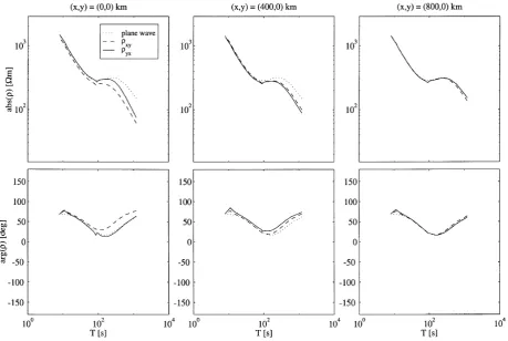
Fig. 13. Absolute values and phases of the apparent resistivitiesρx yandρyxas a function of period atx=0, 400, 800 km (y=0 km) in the case of the omega band. The conductive earth model is used. The plane wave value is plotted as a dotted line.

(11)

Fig. 15. Snapshot of the horizontal current system producing giant pulsations.

(12)

Appendix. Field of an Eastward Elementary

Cur-rent

Consider an electrojet of afinite length, having vertical currents at both ends. Assume that the horizontal current

flows from (x0,y0,−h) to (x0,y1,−h), a downward

cur-rent ends at (x0,y0,−h), and an upward current starts at

(x0,y1,−h). The amplitude of the current isI, and the

an-gular frequency isω.

The complex image depth is (Boteler and Pirjola, 1998; Pirjola and Viljanen, 1998)

p= p(ω)= Z(ω) iωμ0

(A.1)

where the plane wave surface impedanceZcan be calculated from a recursion formula (cf. Wait, 1981, pp. 52–53).

The primary magnetic and electricfields at the earth’s sur-face due to the horizontal currentfilament are

Bx p(x,y)= −

secondaryfields are obtained by replacingh withh+2p, and changing the sign ofBzpandEyp.

The primaryfield due to the radial horizontal current that is equivalent to the downward current at (x0,y0,−h) is

see Pirjola and Viljanen, 1998). Bzpis zero. The secondary field is obtained by replacinghwithh+2p, and changing the sign of the electricfield. Formulas for the upward current at (x0,y1,−h) are obtained similarly by replacing (x0,y0) with

(x0,y1) and changing the signs.

Formulas for thefields produced by a northwardfilament are obtained in an obvious manner from Eqs. (A.2) and (A.3) by a rotation of the coordinate system.

References

Amm, O., Direct determination of the local ionospheric Hall conductance distribution from two-dimensional electric and magneticfield data: Ap-plication of the method using models of typical ionospheric electrody-namic situations,J. Geophys. Res.,100(A11), 21473–21488, 1995. Amm, O., Improved electrodynamic modeling of an omega band and

anal-ysis of its current system,J. Geophys. Res.,101, 2677–2683, 1996. Boteler, D. H. and R. J. Pirjola, The complex-image method for calculating

the magnetic and electricfields at the surface of the Earth by the auroral electrojet,Geophys. J. Int.,132, 31–40, 1998.

Chave, A. D., D. J. Thomson, and M. E. Ander, On the robust estimation of power spectra, coherences, and transfer functions,J. Geophys. Res.,92, 633–648, 1987.

Egbert, G. D. and J. R. Booker, Multivariate analysis of geomagnetic array data. 1. The response space,J. Geophys. Res.,94, 14227–14247, 1989a. Egbert, G. D. and J. R. Booker, Multivariate analysis of geomagnetic array data. 2. Random source models,J. Geophys. Res.,94, 14249–14265, 1989b.

Garcia, X., A. D. Chave, and A. G. Jones, Robust processing of magnetotel-luric data from the auroral zone,J. Geomag. Geoelectr.,49, 1451–1468, 1997.

Glassmeier, K.-H., Magnetometer array observations of a giant pulsation event,J. Geophys.,48, 127–138, 1980.

Hakkinen, L. and R. Pirjola, Calculation of electric and magnetic¨ fields due to an electrojet current system above a layered earth,Geophysica,22, 31–44, 1986.

Hakkinen, L., R. Pirjola, and C. Sucksdorff, EISCAT magnetometer cross¨

and theoretical studies connected with the electrojet current system, Geo-physica,25, 123–134, 1989.

Korja, T. and the BEAR Working Group, BEAR. Baltic Electromagnetic Array Research,EUROPROBE News, No. 12, 4–5, 1998.

Larsen, J. C., R. L. Mackie, A. Manzella, A. Fiordelisi, and S. Rieven, Robust smooth magnetotelluric transfer function,Geophys. J. Int.,124, 801–819, 1996.

Mareschal, M., Modelling of natural sources of magnetospheric origin in the interpretation of regional induction studies: a review,Surv. Geophys., 8, 261–300, 1986.

Osipova, I. L., S. E. Hjelt, and L. L. Vanyan, Sourcefield problems in northern parts of the Baltic Shield,Phys. Earth Planet. Inter.,53, 337–

342, 1989.

Padilha, A. L., I. Vitorello, and L. Rijo, Effects of the Equatorial Electrojet on magnetotelluric surveys: Field results from Northwest Brazil,Geophys. Res. Lett.,24, 89–92, 1997.

Pirjola, R., On magnetotelluric source effects caused by an auroral electrojet system,Radio Sci.,27(4), 463–468, 1992.

Pirjola, R. and A. Viljanen, Complex image method for calculating electric and magneticfields produced by an auroral electrojet of afinite length, Ann. Geophys.,16, 1434–1444, 1998.

Pirjola, R., D. Boteler, A. Viljanen, and O. Amm, Prediction of geomagnet-ically induced currents in power transmission systems,Adv. Space Res., 1999 (accepted for publication).

Szarka, L. and G. Fischer, Electromagnetic parameters at the surface of a conductive halfspace in terms of the subsurface current distribution, Geophysical Transactions,25(3), 157–172, 1989.

Thomson, D. J. and J. T. Weaver, The complex image approximation for induction in a multilayered Earth,J. Geophys. Res.,80(1), 123–129, 1975.

Untiedt, J. and W. Baumjohann, Studies of polar current systems using the IMS Scandinavian magnetometer array,Space Science Reviews,63, 245–390, 1993.

(13)

A. VILJANENet al.: SOURCE EFFECT STUDIES WITH THE COMPLEX IMAGE METHOD 945 Viljanen, A., Source effect on geomagnetic induction vectors in the

fennoscandian auroral region,J. Geomag. Geoelectr.,48, 1001–1009, 1996.

Viljanen, A. and R. Pirjola, On the possibility of performing studies on the geoelectricfield and ionospheric currents using induction in power systems,J. Atmos. Terr. Phys.,56, 1483–1491, 1994.

Viljanen, A., R. Pirjola, and L. H¨akkinen, An attempt to reduce induction source effects at high latitudes,J. Geomag. Geoelectr.,45, 817–831, 1993. Wait, J. R.,Wave Propagation Theory, 348 pp., Pergamon Press, 1981.

Wait, J. R. and K. P. Spies, On the representation of the quasi-staticfields of a line current source above the ground,Can. J. Phys.,27, 2731–2733, 1969.

Weidelt, P., The Inverse Problem of Geomagnetic Induction,Z. Geophys., 38, 257–289, 1972.