FULL PAPER
Statistical analysis of geomagnetic field
intensity differences between ASM and VFM
instruments onboard Swarm constellation
Paola De Michelis
1*, Roberta Tozzi
1and Giuseppe Consolini
2Abstract
From the very first measurements made by the magnetometers onboard Swarm satellites launched by European Space Agency (ESA) in late 2013, it emerged a discrepancy between scalar and vector measurements. An accurate analysis of this phenomenon brought to build an empirical model of the disturbance, highly correlated with the Sun incidence angle, and to correct vector data accordingly. The empirical model adopted by ESA results in a significant decrease in the amplitude of the disturbance affecting VFM measurements so greatly improving the vector magnetic data quality. This study is focused on the characterization of the difference between magnetic field intensity meas-ured by the absolute scalar magnetometer (ASM) and that reconstructed using the vector field magnetometer (VFM) installed on Swarm constellation. Applying empirical mode decomposition method, we find the intrinsic mode func-tions (IMFs) associated with ASM–VFM total intensity differences obtained with data both uncorrected and corrected for the disturbance correlated with the Sun incidence angle. Surprisingly, no differences are found in the nature of the IMFs embedded in the analyzed signals, being these IMFs characterized by the same dominant periodicities before and after correction. The effect of correction manifests in the decrease in the energy associated with some IMFs contributing to corrected data. Some IMFs identified by analyzing the ASM–VFM intensity discrepancy are character-ized by the same dominant periodicities of those obtained by analyzing the temperature fluctuations of the VFM electronic unit. Thus, the disturbance correlated with the Sun incidence angle could be still present in the corrected magnetic data. Furthermore, the ASM–VFM total intensity difference and the VFM electronic unit temperature display a maximal shared information with a time delay that depends on local time. Taken together, these findings may help to relate the features of the observed VFM–ASM total intensity difference to the physical characteristics of the real disturbance thus contributing to improve the empirical model proposed for the correction of data.
Keywords: Swarm magnetic data quality, Empirical mode decomposition, Delayed mutual information
© The Author(s) 2017. This article is distributed under the terms of the Creative Commons Attribution 4.0 International License (http://creativecommons.org/licenses/by/4.0/), which permits unrestricted use, distribution, and reproduction in any medium, provided you give appropriate credit to the original author(s) and the source, provide a link to the Creative Commons license, and indicate if changes were made.
Background
The Swarm mission, which consists of three identi-cal satellites, was launched on November 2013 by the European Space Agency (ESA) with the objective to perform the best-ever survey of the geomagnetic and electric fields surrounding the Earth (Friis-Christensen et al. 2006). The three satellites fly on almost polar orbits (inclination being around 88◦
) and are equipped with
identical magnetometers and electric field instruments capable of providing high-precision and high-resolution measurements.
One of the peculiar features of Swarm mission is the geometry of the satellite constellation. Two satellites, Alpha (A) and Charlie (C), fly in pair at an altitude that on August 2016 was approximately of 460 km. The third satellite, Bravo (B), orbits about 50 km above Swarm A and C, and it is constantly increasing its local time (LT) separation from A and C. This separation was of about 3 h on August 2016. Further details on Swarm mission can be found at http://swarm-wiki.spacecenter.dk/medi-awiki-1.21.1/index.php/Swarm_User_Guide.
Open Access
*Correspondence: [email protected]
1 Istituto Nazionale di Geofisica e Vulcanologia, Roma, Via di Vigna Murata 605, 00143 Rome, Italy
Magnetic measurements on each satellite are carried out by an absolute scalar magnetometer (ASM) for meas-uring Earth’s magnetic field intensity and by a vector field magnetometer (VFM) for measuring the direction and the strength of the geomagnetic field. VFM measure-ments are calibrated using those from the ASM similarly as already done in other satellite missions for magnetic field mapping purposes and which carried equivalent instrumentation (Olsen et al. 2003; Yin and Lühr 2011). According to the traditional in-flight vector calibration of VFM fluxgate instruments, the raw data of the vec-tor magnetometer are processed by applying an error model which takes into account of scale factors and their dependence on time and temperature, offsets and non-orthogonal angles between the sensor elements.
From the very beginning of the Swarm mission, com-parisons between magnetic measurements from VFM and ASM showed discrepancies in the values of total field intensity which could not be captured by the tradi-tional in-flight calibration methods. These differences were observed in data of all satellites appearing as a disturbance in magnetic field measurements varying in strength, direction and characterized by a local time dependence. A first investigation on VFM and ASM measurements suggested that this disturbance was due to an unforeseen spurious magnetic field that contaminated the VFM measurements more than ASM ones. Succes-sively, a comparison of ASM measurements recorded by all satellites during specific satellites maneuvers showed that the origin of this disturbance, and hence of the observed ASM–VFM total field differences, was not to be ascribed to the ASM. For this reason, it was decided to assume that only the VFM measurements had to be cor-rected for the presence of this undesired magnetic field whose indirect cause was attributed, after some investi-gations on ASM–VFM total field differences, to some thermal effect due to the varying Sun incidence angle with respect to the spacecraft.
To correct VFM measurements and consequently reduce the discrepancy between VFM and ASM total intensity of the magnetic field, a correction model was proposed (Lesur et al. 2015). This model is capable of reconstructing the vector components of the disturbing magnetic field and therefore of correcting the single vec-tor components provided by the VFM. The model con-sists of a spherical harmonics expansion up to degree and order 25 in the Sun incidence angle whose coefficients are estimated iteratively by means of a least squares method. This empirical determination of the Sun-driven distur-bance field and its consequent removal have become part of the in-flight calibration of the Swarm ensemble of magnetometers (Tøffner-Clausen et al. 2016). Being this disturbance field different for each satellite, coefficients
are estimated separately for the three satellites. The final effect of correction on magnetic vector measurements for all Swarm satellites is quite good and substantially reduces the standard deviation of the difference between ASM and VFM geomagnetic field total intensity. The occasional spikes that are present in corrected data cor-respond to satellite maneuvers that the model is not able to represent.
Detailed descriptions of the correction model can be found in the ESA technical report available at https:// earth.esa.int/documents/10174/1583357/Prelimi-nary_Swarm_MagL_Data_ReleaseNotes and in Tøffner-Clausen et al. (2016).
To try to gain additional information on the distur-bance affecting magnetic measurements and on the way correction acts on magnetic vector data, we perform an analysis based on empirical mode decomposition (EMD) method. We apply this method to the ASM–VFM total intensity differences obtained with data both uncorrected and corrected for the disturbance correlated with the Sun incidence angle, and we try to understand the nature of disturbance which, despite correction, is still partially present in VFM measurements. For this reason, we analyze also the VFM electronic unit temperature time series, which can be used as a proxy of how the tempera-ture changes in the satellite environment along its orbit.
It is important to keep in mind that each time a cor-rection is applied on a measurement there is a real risk to introduce spurious features that could be turned into spurious properties of the analyzed corresponding time series and, consequently, into incorrect physical inter-pretation of results provided by the analyses performed on manipulated data. Due to the very large community interested in Swarm data, from those studying the slow evolution of the Earth’s core to those interested in the very quickly changing magnetospheric/ionospheric envi-ronment, it is important to be aware of the effects, if any, of the performed correction. It can be important to know whether there are timescales more affected than others.
The present work is intended to provide a characteri-zation of the nature of the residual discrepancy of the ASM–VFM total intensity measurements to understand the linear/nonlinear and/or chaotic nature of this spuri-ous signal, leaving the discussion on any possible solution to this problem to further investigations which require a deeper knowledge of mechanical and electronic fea-tures of the two instruments. We retain that our results can give useful information to all people that work to improve the quality of Swarm magnetic data and have the right skill to try to solve the problem.
applied to the selected Swarm dataset. Results from the application of EMD are displayed and discussed in the same section. Then there is a section where delayed mutual information is illustrated and applied to our data-set. In “Summary and conclusions” section, main findings are summarized and implications discussed.
Data
We consider Level 1b low-resolution (1 Hz) magnetic field data recorded onboard Swarm constellation. In detail, we use two different data groups: one consists of the difference between the total magnetic field intensity provided by the two magnetic instruments (ASM and VFM) installed onboard the three satellites from May 15, 2014, to September 12, 2014, the other one consists of both ASM–VFM total field difference and VFM elec-tronic unit temperature recorded from January 13, 2015, to June 29, 2015, by Swarm B. Magnetic measurements used to calculate ASM–VFM total field differences are contained in files named SW_OPER_MAGx_LR_1B (x = A, B, C) and are available at ftp://swarm-diss.eo.esa. int upon registration.
In the first data group, we use both uncorrected and corrected data. Following ESA archiving nomenclature, we will refer to uncorrected data as Previous (file counter equal to 0301, 0302 and 0303) and �FP(t) will be the cor-responding series of ASM–VFM total field differences. Similarly, we will refer to corrected data as Current and �FC(t) will be the corresponding series of ASM–VFM total field differences. We want to draw the reader’s attention that according to ESA nomenclature the most recent data version is named Current version but this has changed in the course of the investigation presented in this paper. For instance, as far as concerns magnetic data, at the time of the investigation performed on the first data group, i.e., July 2015, Current data consisted of files with file counter equal to 0405. Differently, as explained later on, at the time of the investigation on the second data group, i.e., February 2016, Current magnetic data consisted of files with file counter equal to 0408.
The standard deviation of ASM–VFM total field differ-ences, obtained by Previous data, covering the analyzed period ranges between 0.7 and 1.3 nT (the maximum value being reached by Swarm A). When standard devia-tion is estimated on Current data (0405), it drops to val-ues between 0.15 and 0.19 nT.
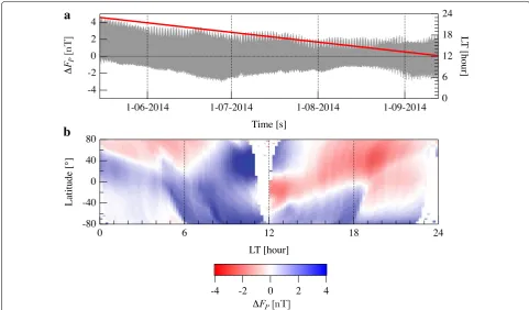
Before performing any analysis, data have been deci-mated to reduce the number of values, and therefore, 1 value every 10 s is considered. Figures 1 and 2 present an example of the analyzed time series relative to the first data group in the case of Swarm A from May 15, 2014, to September 12, 2014. Both figures show on the top the temporal trend of the analyzed difference (�FP(t) in
Fig. 1 and �FC(t) in Fig. 2) and on the bottom a map of its local time (LT) distribution. Being the characteristics of ASM–VFM differences dependent on local time, the local time of the ascending node of the satellite during the analyzed period is also drawn in these figures.
Concerning magnetic field measurements used in the second data group, we consider only the corrected ver-sion, as mentioned above in this case Current data con-sist of files with file counter equal to 0408, to estimate the ASM–VFM differences [�F(t)]. Figure 3 shows the sec-ond data group: �F(t) and VFM electronic unit tempera-ture (TEU) in the time interval January 13, 2015–June 29,
2015, recorded onboard Swarm B satellite.
As in the case of magnetic data also the set of data describing the VFM electronic unit temperature is a Swarm Level 1b product available upon registration at ESA ftp. Measurements used in this work are contained in common data format (CDF) files named MAGB_ CA_1B with file counter equal to 0407, the most recent version available on February 2016. Besides magnetic data (raw as well as processed VFM vector measurements and fully converted and corrected ASM measurements), these files contain VFM electronic unit and sensors tem-peratures. In the CDF files, electronic unit temperature corresponds to T_EU variable, while sensor tempera-tures correspond to T_CDC and T_CSC variables (CDC and CSC stand for Compact Detector Coil and Compact Spherical Coil, respectively).
Empirical mode decomposition analysis: a brief account and results
Data describing the dynamics of both natural and man-made systems are often characterized by a certain degree of non-stationarity and nonlinearity. This is the reason why, to describe the dynamics of these systems, it is nec-essary to introduce methods of analysis different from the traditional ones usually based on assumptions of lin-earity and stationarity of the analyzed time series. These different analytical methods are capable of represent-ing the inherent multi-scale and complex nature which characterizes the systems permitting us to gain a deep understanding of those physical processes which actually produce data. Moreover, they decompose signals using adaptive bases that are directly derived by data them-selves without setting a priori assumptions.
been applied in different physical contexts from seismol-ogy (Battista et al. 2007) to oceanography (Schlurmann
2000, 2002) without considering the applications in bio-medical signal processing (Pachori 2008) and in signal denoising (Flandrin et al. 2004).
EMD has been widely used also in geomagnetism, for example to characterize the decadal periodicities of the length of the day and find a relation with torsional oscil-lations (Roberts et al. 2007; Jackson and Mound 2010; De Michelis et al. 2013), to study the multi-scale nature of geomagnetic storms (De Michelis et al. 2012, 2015) and to analyze their impact on electric power systems (Liu et al. 2016).
The main idea behind EMD is that any time-dependent data series can be written as a superposition of mono-component signals each representing characteristics embedded in the time-dependent data series. These monocomponent signals, named intrinsic mode func-tions (IMFs), can be directly extracted from the original time series, provided that they satisfy two important con-ditions. The first condition requires that number of zero crossings and of extrema are equal or differ by at most one. The second condition requires that the mean value of the two envelops fitting IMF local maxima and local minima is
equal to zero. This second condition, which means that the local mean of IMF is equal to zero and guarantees that the instantaneous frequency will not have unwanted fluctua-tions, represents the new idea of the method. To decom-pose a signal via EMD, an iterative procedure must be followed. We do not describe here the details of this pro-cedure since they are reported in many scientific papers (Huang et al. 1998, 2003; Huang and Wu 2008; Flandrin et al. 2004; De Michelis et al. 2012). This iterative proce-dure ends in a number of IMFs and a residue representing the long-term trend of the analyzed time series. IMFs, due to the way they are built, have each a characteristic fre-quency and become the basis representing the data, which is consequently obtained with no a priori assumptions on the time-series nature. IMFs can have both frequency and amplitude modulations. A wave component with nearly constant time scale exists and dominates in each IMF, rep-resenting the carrier wave constituent at the specific time scale. In this way, we are capable of identifying the differ-ent IMFs which correspond to the differdiffer-ent physical time scales and characterize the various dynamical oscillations in the analyzed time series.
Here, we apply EMD to discern the timescales which characterize the difference between measurements of
a
b
intensity of the Earth’s magnetic field made indepen-dently by the scalar and the vector magnetometers (ASM and VFM). This time-dependent data series is
non-stationary and may result from nonlinear processes. This is the reason why it is important to choose an anal-ysis tool like EMD. In respect of the standard methods
a
b
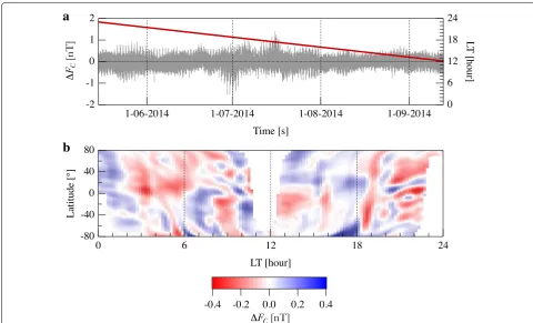
Fig. 2 First data group: fragment of Current dataset. a Plot of the difference FC between the Earth’s magnetic field total intensity measured by the ASM and that reconstructed using the VFM. Local time of the ascending node of the satellite is reported on the right axis in red; b map of LT distribution of FC. Current data are corrected for the disturbance correlated with Sun incidence angle; values consist of decimated low-resolution magnetic measurements recorded from May 15, 2014, to September 12, 2014, by Swarm A satellite
such as FT (Fourier transform) or MEM (maximum entropy method), the advantage of this procedure is that it is the most mathematically correct procedure for the time series here analyzed. The risk of using the above-mentioned standard methods is that they can produce spurious components which might make mathematical sense but not a physical sense. Thus, EMD is not only a useful method but possibly the only computational method of analysis for nonlinear and non-stationary signals.
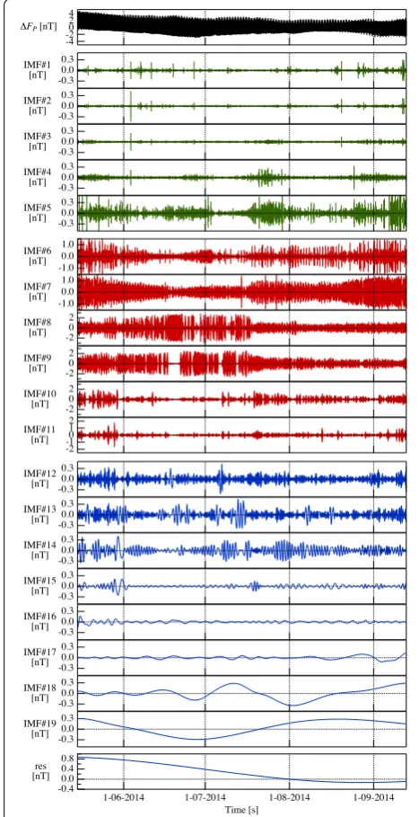
We start by analyzing the difference FP obtained con-sidering uncorrected measurements recorded by Swarm A from May 15, 2014, to September 12, 2014. Figure 4
shows the complete decomposition of FP. Here, IMFs are displayed in different colors (green, red and blue) to underline the different way they contribute to the total signal (the criterion used for this separation is explained in the following). The time series is decomposed into 19 IMFs, and a residue and can be written as follows:
A general separation of FP time series into locally non-overlapping timescale components with varying ampli-tudes is found. Recent studies by Flandrin et al. (2004) and Wu and Huang (2004) have established that the IMFs components are usually physically meaningful. Therefore, an accurate analysis of the IMFs may help us to understand the nature of the processes responsible of the observed differences on different timescales. The total number of the obtained IMFs is well in agreement with the expected number for signals characterized by a large number of scales such as colored noises and tur-bulence. In these cases, the expected number of IMFs is approximately equal to log2N, where N is the total number of data points. Containing FP about 106 points, the expected number of IMFs is between 19 and 20. Of course, not all IMFs contribute with the same energy to the overall signal.
Although we have defined IMFs as monocomponents, in practice their frequency content spreads over a (small) band of frequencies, so to characterize each IMF in terms of signal energy and dominant period, the mean frequency and the associated energy of each IMF must be evaluated. For this reason, in order to identify which of the intrinsic modes contributes most strongly to the original signal, we estimate the energy of each IMF (in terms of its variance) and study its dependence on the mean frequency associated with each IMF. Once energy and mean frequency are estimated, we characterize the carrier wave constituent of the signal at the specific time scale. The estimation of the mean frequency of each IMF (1)
can be computed by means of the associated Fourier power spectral density (PSD) Sk(f) using the following
expression:
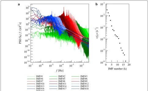
Figure 5 shows, on the left panel, the Fourier PSD for each IMFk (k=1,. . ., 19) reported with shades of red, green and blue according to Fig. 4, while on the right it displays the corresponding mean frequencies <fk > evaluated according to Eq. (2) as a function of the mode number k. Looking at this trend (<fk> vs k reported on the right panel of Fig. 5) it is evident that the IMFs provide a frequency response similar to that of a dyadic filter bank (Flandrin et al. 2004). It has been found that IMFs tend to mimic a filter bank structure, similar to that observed in the case of wavelet decom-positions (Flandrin et al. 2004; Wu and Huang 2004), where filter banks represent a collection of band-pass filters designed to isolate different frequency bands in the input signal. However, the filter bank structure from EMD is completely self-adaptive with respect to Fourier and/or wavelet filtering methods.
Figure 6a provides the energy of each IMFk as a func-tion of the corresponding IMFk mean frequency <fk > . The different colors (green, blue and red as in Fig. 4) identify the different way IMFs contribute to the analyzed signal, i.e., FP. Indeed:
1. the modes with k = 1, ..., 5 (green) describe the noise associated with the signal containing 0.2% of FP
total energy,
2. the modes with k = 6, ..., 11 (red) contain 92% of FP
total energy and, consequently, the signal obtained by the superposition of these modes represents the main part of FP and is well representative of the
ASM–VFM differences:
3. remaining modes (k = 12, ..., 19) (blue) take into account the remanent part of the signal
Figure 6b shows a small sample of data reported on the top of Fig. 1 (FP) and the comparison with the differ-ent signals reconstructed using Eqs. (3), (4) and (5). The analyzed time interval is of approximately 7 h. The main signal (MainP) obtained considering the superposition of six IMFk (k=6,. . ., 11) is well in agreement with the original signal (FP). The frequency band associated with MainP, i.e., f6≤f ≤f11, is that playing the key role in the description of FP. So, we expect that this is the
frequency band associated with the sources producing the spurious magnetic field affecting VFM measurements and preventing ASM and VFM measurements from being equal or, as expected, from differing by a signal similar to a white noise.
We now use the same working scheme on FC to verify whether this same frequency band plays a key role also in the corrected data (Current data). In this case, the time series FC relative to Swarm A satellite is decomposed into 20 IMFs and a residue as follows:
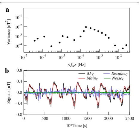
As in the Previous case, we evaluate the mean fre-quencies associated with each IMFk and we report the value of the variance associated with each IMFk as func-tion of the corresponding mean frequency <fk > in Fig. 7a. When comparing Figs. 6a and 7a, two aspects must be focused: absolute values of energy and their distribution with frequency. As regards the first aspect, we observe that correction has significantly reduced the energy associated with the different modes embedded in the two analyzed signals. As regards the second aspect, we see that the energy distribution with frequency does not change so much. If the correction of the Sun-driven disturbance field on VFM data was properly captured, we would expect that mean frequencies of the differ-ence between the intensity of the Earth’s magnetic field measured by ASM and by VFM are distributed more or less as for a white noise. Conversely, we find results similar to those obtained for Previous data. In this case, the first 3 IMFs describe the Noise of the analyzed signal FC:
We recall that when decomposing FP we have found that the MainP signal is given by the superposition of six IMFs [see Eq (4)]. Now, for the Current data (FC) we consider those IMFs which are characterized by mean frequencies in the same frequency band of MainP, i.e.,
f6≤f ≤f11, to check whether the IMFs characterized by these frequencies play a key role also in the case of corrected data. For this reason, in the case of FC data-set, we consider as MainC signal that obtained from the superposition of IMFk with k=7,. . ., 11, therefore:
(6) �FC(t)=
20
k=1
IMFk(t)+res(t).
(7)
NoiseC= 3
k=1
IMFk(t).
(8) MainC=
11
k=7
IMFk(t),
Fig. 4 Example of empirical mode decomposition. From top to
while all the other IMFs describe the remanent part of the signal, that in this case is equal to
A zoom showing a comparison among the original signal FC and the reconstructed NoiseC, MainC and
ResidueC signals is shown in Fig. 7b in the case of Swarm A satellite. Also in this case the zoom permits to visual-ize about 7 h of data. The local time distributions of the reconstructed signals are displayed in Fig. 8. Here, look-ing at MainC we notice that the signal is still spatially structured, which suggests that the disturbance that affects VFM measurements has not been completely removed. Indeed, we would expect that after a proper data correction, the local time distribution should not contain coherent structures as for a white noise. Con-versely, the frequency band, which dominates FP, plays a key role also in FC. The decompositions obtained by the two analyzed datasets are practically the same. The main difference is in the energy associated with Cur-rent data that is about one order of magnitude lower
(9)
ResidueC= 6
k=4
IMFk(t)+ 20
k=12
IMFk(t)+res(t).
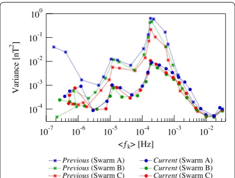
than that associated with Previous data (see panels a of Figs. 6, 7). We have repeated this analysis also in the case of the other two satellites (Swarm B and Swarm C). Fig-ure 9 reports a comparison among the variance associ-ated with each IMFk obtained decomposing FP and FC for the three satellites. The analysis made on the mag-netic data measured from the three satellites (Swarm A, B and C) before the correction for the disturbance cor-related with Sun incidence angle shows that the source of the disturbance is the same and can be described using a superposition of modes with the same mean frequencies, which are, however, characterized by slightly different amplitudes. Looking at the results of Fig. 9, it is possible to conclude that in the case of Previous data the lowest disturbance intensity is experimented by Swarm C. This difference in the data quality among the Swarm satellites is lost after the data correction. The comparison among the variance associated with each IMFk obtained decom-posing FC for the three satellites of Swarm constellation reveals that the three decompositions are practically the same.
In summary, independently from the selected satellite our findings suggest that:
a
b
Fig. 5 Example of PSD. a Fourier power spectral density (PSD) of each IMFk identified in the decomposition of FP for Swarm A and reported in
(a) the modes embedded in the analyzed signals before and after correction are characterized by the same dominant periods;
(b) the main difference consists in the decrease in the energy associated with some modes contributing to corrected data.
It is worth recalling that since we are considering the difference between the magnetic field intensity obtained from the ASM and VFM onboard the same satellite, the common periods in the two original signals should be automatically deleted and what we obtain should describe the effect of the disturbance suffered from VFM meas-urements. Thus, although the disturbance is mainly char-acterized by modes with frequencies close to the orbital period of Swarm satellites (as it is reported in Figs. 6, 7
and 9), these frequencies are not the direct result of satel-lite orbiting the Earth. They are a real feature of the dis-turbance and hence of its source mechanism.
Due to the large number of modes necessary for the description of the disturbance, this could be interpreted in terms of a nonlinear response of the VFM to the vary-ing environmental conditions. Anyhow, some mecha-nisms responsible for the observed disturbance field still exist in the Current data and are not completely removed using the empirical model (Lesur et al. 2015) built to cor-rect VFM measurements.
The correction made on the data resulted in a signifi-cant decrease in the amplitude of the disturbance affect-ing VFM measurements, therefore greatly improvaffect-ing the magnetic vector data quality. However, our findings (see Fig. 9) suggest that the correction actually decreased the amplitude of the difference between ASM and VFM total intensity but, since the origin of the disturbance has not been identified, the spurious magnetic field affect-ing VFM measurements is still present, with less energy but with the same structure as before correction. To try to understand the origin of the disturbance field which still affects data also after the correction, we analyze the second data group described in “Data” section. Our hypothesis is that after correction, VFM magnetic meas-urements are still affected, through a mechanism we do not know, by the effects of different satellite heating due to the varying position of the Sun relative to the satellite. To verify this hypothesis, we check whether the tempera-ture of the VFM electronic unit, which could be consid-ered a proxy of the changes in the satellite environment along its orbit, is decomposed in a similar way as for ASM and VFM total intensity differences obtained from corrected data.
a
b
Fig. 6 Variance and comparison among FP and different recon-structed signals. a Variance associated with each IMFk obtained
decomposing FP plotted as a function of the associated mean frequency <fk>. Colors used in the case of the variance of each IMF correspond to those used in Fig. 4. b A zoom showing a comparison among the original signal FP and the different signals reconstructed using Eqs. (3), (4) and (5), respectively. Data here considered are rela-tive to Swarm A.
a
b
Fig. 7 Variance and comparison among FC and different recon-structed signals. a Variance associated with each IMFk obtained decomposing FC plotted as a function of the associated mean fre-quency <fk>. b A zoom showing a comparison among the original
We apply EMD to the second data group, i.e., both the total field ASM–VFM differences (F) and the electronic unit temperature (TEU) of the VFM (see Fig. 3) onboard
Swarm B. In this case, we consider a time interval longer than the previous one: We analyze about 6 months of data from January 13, 2015, to June 29, 2015. Using this different period, we can verify that our previous results remain valid independently of both the length of the ana-lyzed time series and the specific time period considered. At the same time, we can verify the existence of a pos-sible relation between the observed magnetic disturbance and the temperature changes the VFM has undergone and therefore indirectly the temperature changes of the environment around the satellite. Being the temperature
data available with a time resolution of 15 s, we consider 1 value every 15 s also in the case of magnetic data (F).
By applying EMD to F, we decompose it into 21 IMFs and a residue. The distribution of the energy associated with the obtained modes is consistent with the previous ones, indicating that disturbance field is always charac-terized by the same decomposition regardless of the ana-lyzed period, its length, the used satellite and data version (in this case 0408).
We apply the same method of analysis to the VFM electronic unit temperature data (TEU) and decompose
it into 13 IMFs and a residue as reported in Fig. 10. The total number of modes obtained from the decomposi-tion of TEU data is lower than that obtained in the case
of F . This may be explained by the fact that the num-ber of modes depends partially on the complexity of the analyzed signal, on its information content. Fig-ure 11 compares the variance associated with each IMFk obtained decomposing F and TEU plotted as a function
of the associated mean frequency. What is interesting in these data is that there is a coincidence between some frequency peaks observed in the total field ASM–VFM differences and temperature ones. Indeed, TEU is
decom-posed in a set of IMFs some of which have the same mean frequencies found for F. This observation may support the hypothesis that the disturbance correlated with the Sun position relative to the satellite is still present in the Swarm level 1b corrected magnetic data. We underline that in this case we used data with file counter equal to 0408. This disturbance is responsible of more than 85% of the magnetic field discrepancy as it can be evaluated considering the energy associated with the modes which describe the main part of ASM–VFM differences.
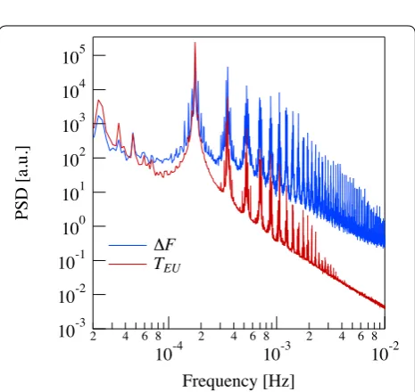
We apply to our time series (TEU and F) the most tra-ditional data processing methodologies such as the Fou-rier transform to examine their global energy-frequency distribution. However, as it is well known that the Fourier transform has been developed under rigorous mathemat-ics rules: the Fourier spectra can only give meaningful interpretation to linear and stationary processes. In all the other cases, the use of Fourier spectral analysis may give misleading results. For instance, in the case of a signal from nonlinear processes to describe the deformed wave profiles which are the direct consequence of nonlinear effects, the Fourier spectral analysis, which is based on a linear superposition of trigonometric functions, needs
additional harmonic components. In particular, a typical signature of a signal resulting from nonlinear process is the existence of subharmonics and super-harmonics in the Fourier power spectrum which occur as integer submul-tiples and mulsubmul-tiples of the fundamental frequency. What happens ultimately is that the non-stationarity and nonlin-earity when they are analyzed using the Fourier transform induce many additional harmonic components spreading the energy over a wide frequency range. This is what hap-pens in our case. The PSDs of the two signals (TEU and F ) are reported in Fig. 12 for a comparison. Of course, since F and TEU describe different physical quantities, to
com-pare them we have subtracted to each series its mean value and divided by the standard deviation. Looking at Fig. 12, we can recognize the signature of nonlinear response and chaotic excitation in the occurrence of subharmonics and super-harmonics. Indeed, the fundamental peak in the Fourier power spectrum relative to both TEU and F time series coincides with the orbital period of Swarm B sat-ellite, which is equal to 5795 s. This peak is preceded by subharmonics which occur at submultiples of the orbital period and followed by super-harmonics which occur at multiples of the orbital period. The presence of subhar-monics and super-harsubhar-monics suggests that both the two signals may result from a nonlinear response to a common external driving (Linsay 1981), which is expected to be intense (Yen 1971). Considering the peak positions in the frequency domain both in the case of TEU time series and
F one, we can observe that the subharmonics appear to specific ratios with respect to the fundamental frequency (f0≃1.7×10⁻⁴Hz). In particular, the observed ratios agree with what is expected in the case of a chaotic sig-nal according to the period-doubling bifurcation process (Hilborn 2004). Figure 13 shows the dependence of sub-harmonic and super-sub-harmonic frequencies on the ratios of the fundamental frequency (f0) for TEU signal. The straight line supports the chaotic nature of the time series and consequently of the physical processes which are at the origin of this signal. The same conclusion can be drawn for the other analyzed time series (F). Indeed, although the magnetic signal PSD shows a greater number of fre-quency peaks than that obtained for the temperature, most of positions of these peaks are at the same frequencies of those for TEU. Furthermore, the greater number of peaks in
the F PSD suggests that F time series is characterized by a more complex/chaotic nature (Hilborn 2004).
Our findings suggest that an external factor, which could be the different position of the Sun relative to the satellite, still influences both the VFM electronic unit temperature and the VFM magnetic measurements which nonlinearly and chaotically respond to this exter-nal disturbance. One possible scenario is that the VFM responds nonlinearly to electronic unit temperature Fig. 9 Variance. Comparison between the variance associated with
each IMFk obtained decomposing FP and FC plotted as a function
of the associated mean frequency <fk> for all the three Swarm
variations, which are related to the position of the Sun, so that to produce biased measurements. Another possible scenario is the one according to which VFM measuring process is perturbed by external temperature variations through some mechanical deformation whose effect could manifest in terms of a spurious magnetic field. In both cases due to the nonlinear response to the external
forcing, the complexity of the magnetic measurements is increased with respect to those of the inducing electronic unit temperature changes, and therefore, they are charac-terized by a higher number of IMFs.
To know whether these two different physical quanti-ties (TEU and F) share some information, we can apply the mutual information theory which is able to measure the relationship between these two quantities. Indeed, the main advantage of the mutual information theory is that, with respect to the linear cross-correlation function, it is able to capture both linear and nonlinear relation-ships between the analyzed time series.
Delayed mutual information
Mutual information (Cover and Thomas 1991; Gray
1990) is a quantity capable of measuring the amount of information shared by two random variables (X and Y) that are sampled simultaneously. Formally, the mutual information HXY between two discrete random variables is defined as:
where pi(X) and pj(Y) are the probability of observing X and Y as independent variables and pij(X,Y) is the joint probability distribution function of observing the couple of values (X, Y). Since HXY quantifies the information shared by two random variables, it is able to measure how much information is communicated in one variable about another. For this reason, when two variables are statis-tically independent, their mutual information is zero. Indeed, for independent stochastic variables the joint probability pij(X,Y)=pi(X)pj(Y), so that HXY =0 . In all other cases, the value of mutual information will be different from zero reaching a maximum value when the two variables are completely dependent variables (such as, for instance, linearly dependent Y =aX+b). Mutual information, which measures the dependence between two variables, is different from the correlation function. It measures the general dependence, both linear and non-linear, between two variables.
Considering a time delay (τ ) between the two random variables, it is possible to extend the mutual information definition introducing another time-dependent quantity, named delayed mutual informationHXY(τ ):
Mutual information is a symmetric measure, and for this reason, it is not able to indicate the direction of (10)
HXY = N
i,j=1
pij(X,Y)ln
pij(X,Y) pi(X)pj(Y)
(11) HXY(τ )=
N
i,j=1
pij(X(t),Y(t+τ ))ln
pij(X(t),Y(t+τ ))
pi(X)pj(Y)
Fig. 11 Variance. Comparison between the variance associated with each IMFk obtained decomposing F and TEU, respectively. The
vari-ance value is plotted as a function of the mean frequency value asso-ciated with each IMFk. Data here considered are recorded onboard
Swarm B satellite from January 13, 2015, to June 29, 2015
information flow. Conversely, the time-delayed mutual information is capable of designating the delay in the shared information between the two variables and can be used as a measure/indication for mutual coupling. It is equivalent to a nonlinear cross-correlation func-tion which is able to capture both linear and nonlinear correlations.
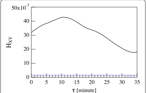
In our case, the two variables X and Y are TEU and F, respectively. Figure 14 displays the delayed mutual infor-mation HXY as a function of τ. There is a maximum in the information shared by the two signals at delay time τ =10.5 min, indicating that there is a delay in the cor-relation between TEU and F. The obtained values of the mutual information and of its maximum are low, but they are significant as shown by the level of significance at the 95% reported in blue in the same figure and obtained
through the bootstrap method (Efron and Tibshirani
1994) applied to the two signals. The bootstrap method is based on the use of the original data to generate a sur-rogate population of samples, where the correlations con-tained in the original one are removed/destroyed. This is obtained by shuffling the original time ordering sample so to create a surrogated sample where internal correlations are removed. This procedure is applied several times so to construct an ensemble consisting of a very large num-ber of surrogated samples. On this ensemble, which in our case consists of 10,000 surrogated samples, one can evaluate the mutual information for each surrogated sam-ple cousam-ple and compute the distribution of the obtained values and the corresponding confidence limit. This method has been applied in our analysis to compute the confidence limit value of the mutual information HXY . In particular, being the distribution of HXY values of the sur-rogated sample Gaussian, we assume the mean value plus 3 standard deviations as confidence limit value of HXY to distinguish correlated from uncorrelated dataset.
As already mentioned, it has been noticed (see, for example, Tøffner-Clausen et al. 2016) that the charac-teristics of ASM–VFM differences depend on local time. For this reason, we extract from magnetic data of the second data group two different time intervals: 5 days (from March 30, 2016, to April 2, 2016) when Swarm B orbits in the dawn–dusk sector and 5 days (from June 25, 2016, to June 29, 2016) when the satellite orbits in the noon–midnight sector (see Fig. 3). Figure 15 displays the two signals during two different days, one for each time interval. The shift between the two signals is not constant but characterized by a dependence on local time. Conse-quently, we can hypothesize that the time delay between the two signals (TEU and F) evaluated using the delayed mutual information may be a function of local time. For this reason, we repeat the analysis of the delayed mutual information considering the time series in the two dif-ferent selected time intervals during which Swarm B orbits in different local time sectors (noon–midnight and dawn–dusk). Figure 16 shows the obtained results. The time delay between TEU and F changes with LT. It is about 6.5 min when the satellite orbits in the noon– midnight sector while it is about 9 min when the satel-lite is in the dawn–dusk sector. Also, in this case we have evaluated the level of significance at 95% through the bootstrap method. Of course, considering the average 10.5 min time delay obtained analyzing a time interval of 6 months, longer time delays are expected in the case of other LTs and perhaps due to seasonal effects. This result suggests that there could be also an anisotropy in the response of VFM instruments on the insolation side.
In conclusion, the delayed mutual information is capa-ble of detecting the delayed shared information between Fig. 13 Subharmonics and super-harmonics in the power spectral
density. Dependence of subharmonic and super-harmonic frequen-cies on the ratios of the fundamental frequency (f0≃1.7×10⁻⁴Hz) in the case of TEU signal
the two time series (TEU and F) without explicitly dis-tinguishing information that is actually exchanged from that due to a response to a common history or common input signal and permitting us to show the existence of a link between TEU and F without providing any informa-tion on whether the correlainforma-tion comes from a linear and/ or nonlinear dependence.
Summary and conclusions
The empirical model for the calibration and correction of the Swarm vector magnetic measurements, introduced by Lesur et al. (2015) and well described in a recent arti-cle by Tøffner-Clausen et al. (2016), has significantly
reduced the scalar residuals between the ASM and VFM measurements of the geomagnetic field greatly improving the magnetic data quality. Indeed, the applied model for the calibration and correction of vector data has reduced to values below 0.5 nT the scalar differences between the Swarm magnetometers. However, the findings related to the analysis of ASM–VFM total field difference seem to suggest that the spurious magnetic field disturbing VFM measurements is still partially present in corrected mag-netic vector data. ASM–VFM difference remains char-acterized by a structure which is different from that of a white noise even after the application of the empirical model for the calibration and correction of the Swarm vector magnetic measurements.
The empirical mode decomposition that we have used as a tool for the characterization of the ASM–VFM total field differences has provided similar decompositions when applied on uncorrected and corrected data. The energy associated with some modes of corrected data is indeed decreased, but the structure of the dependence of the energy associated with each mode on frequency (the same before and after correction) is practically identical. These modes, that explain more than 90% of the observed differences and that we identified as the main modes, exhibit mean frequencies close to the orbital period of satellite. These frequencies are not the result of the typi-cal orbital period which is expected to be contained in the magnetic field measurements. We remind that the analyzed time series are differences of the magnetic field intensity measurements obtained from two different instruments onboard same satellite. This suggests that the discrepancy between the two instruments de facto describes the main features of the magnetic disturbance that we have characterized to gain new information about the possible disturbance sources. A first implication of our results is the possibility that some of the mechanisms responsible for the observed differences between ASM and VFM still affect the Current data regardless of the version used (either 0405 or 0408).
To understand the nature of this remaining residual after the correction of vector magnetic data, we have analyzed the VFM electronic unit temperature data which gives indirect information on the temperature changes recorded by the satellite during its orbit around the Earth. As a result of our analysis, we have found that some of the modes describe the main part of the mag-netic disturbance coincide, in terms of mean frequency values, with modes obtained from the decomposition of the temperature data. This suggests that the different position of the Sun relative to the satellite, which pro-duces temperature changes in the satellite environment, could be still responsible of a small error in the VFM magnetic measurements.
Fig. 15 Comparison between TEU and F signals. From top to bottom
Comparison between TEU (red line) and F (blue line) signals during a day in which the local time of the ascending node of Swarm B is about 12 (Swarm B orbits in the noon–midnight sector) and 18 (Swarm B orbits in the dawn–dusk sector), respectively
The delayed mutual information analysis confirms that there is a shared information between these physical quantities, suggesting that their response to the exter-nal disturbance source is not simultaneous and that it is characterized by a local time dependence. The response of the VFM to the external disturbance source occurs with a delay time of about 10.5 min with respect to the tempera-ture changes of satellite environment when we consider a period of about 6 months where the different position of the satellite with respect to the Sun is not taken into account. The value of the time delay decreases to about 6 min when the satellite orbits in the noon–midnight sec-tor or to about 9 min when it is in the dawn–dusk secsec-tor.
What is interesting to observe is that the delayed shared information between the two signals is found on data corrected by means of the empirical model adopted for the calibration and the correction of the Swarm vector magnetic measurements. These data represent the rema-nent part of the disturbance once its main part, which is expected to be linearly correlated and in phase with the Sun position, has been removed. Thus, we are charac-terizing the residual magnetic disturbance which is the result of nonlinear and chaotic processes as it has been found by analyzing the dependence of the subharmonic and super-harmonic frequencies of the PSD peaks on the ratios/multiples of the fundamental frequency. Indeed, the presence of subharmonics and super-harmonics in the PSD of both the magnetic (F) and temperature
(TEU ) signals suggests that the two signals may result
from a nonlinear response to a common external driving (Linsay 1981) which is expected to be intense (Yen 1971). The obtained values of the time delays give us the oppor-tunity to note that the correlation (linear and/or nonlin-ear) between the magnetic signal and temperature one is stronger when the satellite orbits in the noon–midnight sector than when it is in the dawn–dusk one and that the time of response of the VFM to the temperature changes of the environment around the satellite is a function of local time. For what concerns the observed time delay between the temperature and the magnetic signals, we notice that this time delay is observed on the magnetic field ASM–VFM discrepancy after having removed the Sun-driven disturbance field from vector magnetic meas-urements, so that the long delay could be not surprising. Indeed, if the remanent magnetic discrepancy is repre-sentative of the nonlinear and/or chaotic response of the VFM instrument to the solar irradiance, it could be the result of a long-term thermal drift. This would explain the observed time delay between temperature and magnetic field ASM–VFM discrepancy. Anyway, to our opinion a reasonable possibility for the long time delay observed between temperature and magnetic field discrepancy is that this discrepancy may arise from a nonlinear response
of any mechanical part. Clearly, at this stage this is only a speculation requiring more information on the mechani-cal mounting of the two instruments and on the response of the used material to thermal stress.
The study illustrated above is just an example of a way to try to characterize the difference of total intensity measured by VFM and ASM. Further and deeper investi-gations on the residual distributions and frequency struc-tures are certainly possible and could contribute to relate the features of the observed total intensity residual to the physical characteristics of the real disturbance, thus con-tributing to solve this issue. In this way, it would be pos-sible to improve the model proposed for the correction of data. The effects of correction may be extended beyond the simple reduction in the amplitude of the residual between ASM and VFM. This goal can be achieved, for instance, by analyzing whether and how the estimated mean frequencies change in the time and by analyzing in detail the response, eventually nonlinear, of the VFM to the disturbance source. Another interesting investigation could involve the in-depth study of the dependence of the time delay on local time. Of course, being the remanent disturbance in the vector magnetic measurements mainly due to a nonlinear and chaotic response of the VFM to an external driving process, the task to derive a proper cor-rection algorithm will prove to be very complicated.
Abbreviations
ASM: absolute scalar magnetometer; VFM: vector field magnetometer; ESA: European Space Agency; LT: localtime; EMD: empirical mode decomposition; IMF: intrinsic mode function.
Authors’ contributions
PDM, RT, GC carried out the data analysis and participate in key discussions relative to the physical interpretation of the results. PDM and RT draft the manuscript. All the authors read and approved the final manuscript.
Author details
1 Istituto Nazionale di Geofisica e Vulcanologia, Roma, Via di Vigna Murata 605, 00143 Rome, Italy. 2 INAF-Istituto di Astrofisica e Planetologia Spaziali, Via Fosso del Cavaliere 100, 00133 Rome, Italy.
Acknowledgements
The results presented in this paper rely on data collected by the three satel-lites of the Swarm constellation. We thank the European Space Agency that supports the Swarm mission. The elaborated data for this paper are available by contacting the corresponding author ([email protected]).
Competing interests
The authors declare that they have no competing interests.
Received: 5 August 2016 Accepted: 3 December 2016
References
Cover TM, Thomas JA (1991) Elements of information theory. Wiley, New York De Michelis P, Consolini G, Tozzi R (2012) On the multi-scale nature of large
geomagnetic storms: an empirical mode decomposition analysis. Nonlin-ear Process Geophys 19:667
De Michelis P, Tozzi R, Consolini G (2013) On the nonstationarity of the decadal periodicities of the length of day. Nonlinear Process Geophys 20:1127. doi:10.5194/npg-20-1127-2013
De Michelis P, Consolini G, Tozzi R (2015) Latitudinal dependence of short timescale fluctuations during intense geomagnetic storms: a permuta-tion entropy approach. J Geophys Res Space Phys 120:5633. doi:10.1002 /2015JA021279
Efron B, Tibshirani RJ (1994) An introduction to the bootstrap. Monographs on statistics and applied probability. Chapman & Hall/CRC, London Flandrin P, Rilling G, Goncalvés P (2004) Empirical mode decomposition as a
filter bank. IEEE Signal Process Lett 11:112. doi:10.1109/LSP.2003.821662 Friis-Christensen E, Lürh H, Hulot G (2006) Swarm: a constellation to study the
earth’s magnetic field. Earth Planets Space 58:351
Gray RM (1990) Entropy and information theory. Springer-Verlag, New York Hilborn RC (2004) Chaos and nonlinear dynamics. Oxford University Press,
Oxford
Huang NE, Wu Z (2008) A review on Hilbert–Huang transform: method and its applications to geophysical studies. Rev Geophys 46:RG2006. doi:10.102 9/2007RG000228
Huang NE, Shen Z, Long SR, Wu MC, Shih HH, Zheng Q, Yen NC, Tung CC, Liu HH (1998) The empirical mode decomposition and the Hilbert spectrum for nonlinear and nonstationary time series analysis. Proc R Soc Lond Ser A 454:903
Huang NE, Wu ML, Long SR, Shen SS, Qu WD, Gloersen P, Fan KL (2003) A con-fidence limit for the position empirical mode decomposition and Hilbert spectral analysis. Proc R Soc Lond Ser A 459:2317
Jackson LP, Mound JE (2010) Geomagnetic variation on decadal time scales: what can we learn from empirical mode decomposition? Geophys Res Lett. doi:10.1029/2010GL043455
Lesur V, Rother M, Wardinski I, Schachtschneider R, Hamoudi M, Chambodut A (2015) Parent magnetic field models for the IGRF-12 GFZ-candidates. Earth Planets Space 67:87. doi:10.1186/s40623-015-0239-6
Linsay PS (1981) Periodic doubling and chaotic behavior in a driven anhar-monic oscillator. Phys Rev Lett 47:1349
Liu J, Wang CB, Liu L, Sun WH (2016) The response of òocaò power grid at òow-latitude to geomagnetic storm: an application of the Holbert Huang transform. Space Weather 14:300. doi:10.1002/2015SW001327
Olsen N, Tøffner-Clausen L, Sabaka TJ, Brauer P, Merayo JMG, Jørgensen JL et al (2003) Calibration of the Ørsted vector magnetometer. Earth Planets Space 55:11
Pachori RB (2008) Discrimination between ictal and seizure-free EEG signals using empirical mode decomposition. Res Lett Signal Process. ID 293056: doi:10.1155/2008/293056
Roberts PH, Yu ZJ, Russel CT (2007) On the 60-year signal from the core. Geo-phys AstroGeo-phys Fluid Dyn 101:11. doi:10.1080/03091920601083820 Schlurmann T (2000) The empirical mode decomposition and the Hilbert
spectra to analyze embedded characteristic oscillations of extreme waves. In: Olagnon M, Athanassoulis G (eds) Rogue waves, pp 157–165. Editions Lfremer, ISBN 2-84433-063-0
Schlurmann T (2002) Spectral frequency analysis of nonlinear water waves derived from the Hilbert–Huang transformation. J Offshore Mech Arctic Eng (JOMAE) Am Soc Mech Eng 124:22
Tøffner-Clausen L, Lesur V, Olsen N, Finlay CC (2016) In flight scalar calibration and characterisation of the Swarm magnetometry package. Earth Planets Space 68:129. doi:10.1186/s40623-016-0501-6
Wu Z, Huang NE (2004) A study of the characteristics of white noise using the empirical mode decomposition method. Proc R Soc A 460:1597. doi:10.1098/rspa.2003.1221
Yen N-C (1971) Subharmonic generation in acoustic systems. Tech. Rep, DTIC document