R E S E A R C H
Open Access
Research on distribution route with time
window and on-board constraint based on
tabu search algorithm
Chenglin Ma
*, Yanyan Yang, Lihai Wang, Chu Chu, Chao Ma and Lihua An
Abstract
In order to solve the problem of the optimization of delivery and pickup cargoes’ routes with time windows under the constraints of load and road, the method and algorithm were designed and researched based on these factors. Firstly, the model was built with the constraints of truck number, load quality, load capacity, maximum distance, and customer service time in order to minimize the transportation cost and time cost. Then, the Floyd Algorithm was used to determine the moving path and the shortest distance between each point with the road constraint. 0-1 integer programming method was used to determine the number and type of vehicles. Tabu search algorithm was used to determine the order of delivery and pickup points and the distribution route based on the influence of job requirements of pickup cargoes, the time cost, and the transportation cost. Finally, the case was given to verify the effectiveness of the proposed method. This method can be used to improve the efficiency of delivery and pickup cargoes and the level of distribution service.
Keywords: Tabu search algorithm, Time window, Distribution path planning, Road constraints
1 Introduction
As the distribution of e-commerce is increasing, how to use the distribution information platform to analyze the data and optimize the distribution path becomes more and more important [1]. The distribu-tion process has become more complex, because it includes not only the delivery process, but also the pickup process. The pickup information by radio communication is random, which changes the original distribution plan and increases the complexity of dis-tribution. The multi-objective model constructed by Zheng and Cheng and Song et al. took into account the influence of the distribution service level on the distribution line, but the road constraints encountered in the distribution process were not taken into
ac-count [2, 3]. Li et al., Wen and Shen, and Ding and Jiang proposed the solution of distribution lines based on road constraints, but they lacked the consideration of the customer service level and load restrictions [4– 6]. Li et al., Weng et al., Bie and Li, Bülent, Olcay et al., and Yong et al. had proposed solutions to plan the route of cargo delivery, but they had not taken into account the problem of on-board restrictions on the delivery of cargoes [7–15]. Based on various scholars’ valuable research, this paper studied a distri-bution route planning problem with time windows and the constraints of delivery and pickup cargoes’ process, load and roads. The twice tabu search algo-rithm was designed based on the Floyd Algoalgo-rithm and 0-1 integer programming algorithm by MATLAB software. Finally, an example was used to validate the method in determining the delivery and pickup se-quence and route planning.
* Correspondence:[email protected]
College of Engineering and Technology, Northeast Forestry University (NEFU), Xiangfang Dist. Hexing Rd., Harbin, People’s Republic of China
2 Methodology
2.1 Analysis of the problem
The known values which including the truck total quan-tity, each truck maximum load, each truck maximum distance for distribution, the geographic information of intersection and delivery and pickup cargoes, volume and weight of cargoes were defined based on the infor-mation system of distribution center.
The specific conditions of the model were as follows:
(1) Each truck started from the distribution center and reached each customer along a route back to the distribution center.
(2) Delivery cargo trucks followed the road that is not across the building.
(3) The road was a two-way road.
(4) The cargo volume was less than the rated load capacity of the truck (considering the load condition of flexibility, the rated load capacity of the truck would be multiplied by the factor 0.8). (5) The cargo weight was less than the rated load of
delivery trucks not including the driver weight (assuming the driver weight is 60 kg).
(6) The total volume and weight of the cargoes were less than the rated capacity of all the trucks. (7) The number of express staff was greater than or
equal to the number of delivery trucks.
(8) According to the separation principle of delivery and pickup parcels, it was possible to carry out the pickup cargoes’work only when the spare capacity of the delivery truck exceeded half of its rated load capacity.
2.2 Establishment of mathematical model 2.2.1 Determination of objective function
The objective function was proposed to minimize the sum of transportation costs and time costs in the case of ensuring constraints.
m inZ¼OþP
where O is the transportation cost in the distribution process andPis the total time cost.
The transport cost function was as follows:
O¼X
whereS is the location set, H is the customer location set, V is the truck set, Xijk means truck k was from location i to customer j, Cijk means unit transport cost of truck k from location i to location j, and dij -means the shortest distance between location i and location j.
The time penalty function was as follows:
pkð Þ ¼ti
The time cost was:
P¼X
i∈H
X
k∈V
pkð Þti
The variables in the model were explained as follows:
pk(ti) is the penalty cost because truck k serviced cus-tomerion timeti; tiis the time when the truck actually arrived at the customer site; c1,c2 were the maximum penalty cost because the truckkwas early or late to ser-vice customer i;a1,a2are the positive coefficients of the penalty cost of the early or late arrival of the truck, which reflected the importance of time to customers;T1 is the starting point of time window when customer i
was served; T2 is the end point of time window when customeriwas served.
2.2.2 Constraint description
Each customer was serviced by only one truck. X
i∈S
X
k∈V
Xijk¼1;j∈H ð1Þ
When the free volume of the truck exceeded half of its rated load capacity, it could only carry out the service of pickup cargoes.
The delivery cargoes’ volume could not exceed the rated load capacity.
The delivery cargoes’ weight should not exceed the rated load capacity.
The volume of the delivered cargoes should not exceed the rated load capacity.
X
i∈S
X
j∈F
qjXijk≤Wk;k∈V: ð5Þ
X
i∈S
X
j∈F
hjXijk≤Mk;k∈V: ð6Þ
Each truck only reached one customer at one time.
X
i∈S
Xijk ¼Yik;j∈H;k∈V ð7Þ
It was not allowed that the truck returned to the dis-tribution to pick up the cargoes during the delivery.
Uik−UjkþNXijk≤N−1;i∈S;j∈H;k∈V ð8Þ
It was ensured that the total distance of the truck did not exceed its maximum driving range.
X
i∈S;j∈H
Xijkdij≤Dk;k∈V: ð9Þ
Xijk ¼0;1;i∈S;j∈H;k∈V ð10Þ
Yik¼0;1;i∈S;k∈V: ð11Þ
The variables in the model were explained as follows:
Qis the distribution address set before the start of the pickup cargoes,Eis the distribution address set after the pickup cargoes,Nis the distribution address set,Fis the pickup address set, Xilkpresents whether the cargoes were transported from locationito locationlby truckk,
hjis the cargoes’quality of customerj,qjis the cargoes’ volume of customerj,Mk is the maximum load capacity of truckk, Wkis the load space of truckk,Yik is whether truck kserviced the distribution point, Uik is the access order of customer ion the driving route of truck k, Uik is the access order of customerjon the driving route of truck k, and Dk is the maximum driving distance of truckk.
2.3 Solution of model
2.3.1 Algorithm for solving the problem
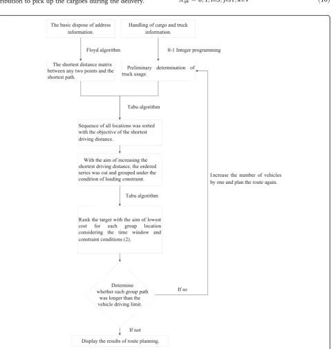
Step structure of algorithm solution is shown in Fig. 1. Firstly, the Floyd Algorithm was adopted to determine the shortest distance path of any two points under the road restraints using address information. Meanwhile, we adopted the 0-1 integer programming to combine the truck and goods information to determine the real-time truck usage, which we called itkl.
Secondly, the access from one distribution center back to the same distribution center was calculated by a tabu search algorithm for the first time with the target of minimizing the driving distance.
Thirdly, the access was randomly divided to match kl
parts; each part must ensure that the corresponding truck could load the delivery goods and pickup goods separately. By calculating the numerical value of the tance between the first item of subsequence and the dis-tribution center by adding the distance between subsequence tail and the distribution center and sub-tracting the distance between each subsequence, the minimum numerical value condition was selected as the optimal grouping.
Then, in consideration of the delivery and pickup rule and the time window, the second time tabu search algo-rithm was used to optimize each sequence in the
optimal group with the fixed distribution center as the first and last member of the sequence aiming at minim-izing the cost.
Finally, we examined whether the total distance of the traveling path to each sequence exceeded the rated driving limit of the truck. If it exceeded, we in-creased the quantity of truck used by one and the so-lution should be re-planned. Else, the optimization result will be displayed.
2.3.2 Initial optimization of distribution path
Step 1: Reading the coordinate information of cargo ad-dress and road intersections was marked as distribution path points by the Arabic numeral. The distance was calculated between cargo address and other cargo ad-dress, cargo address and intersection, and intersection and another intersection.
Step 2: The shortest driving distance was calculated and the driving path was recorded.
(1) Determine the shortest driving distance.
The matrix path represented the shortest distance between any two points of the n × n matrix. The shortest distance between two points was calculated by the Floyd Algorithm. If the shortest distance be-tween two points was not past the third point, the corresponding element of the matrix was the column
Table 1Street/road numbering (part)
Street Numbering
(north-south)
Road Numbering
(east-west)
Tieshun Street 1 Hexing Road 1
Tielu Street 2 Ngbin Alley 2
Second Kangning Street
3 First Hexing Street 3
Table 2Information on street/road junctions (part)
Intersection
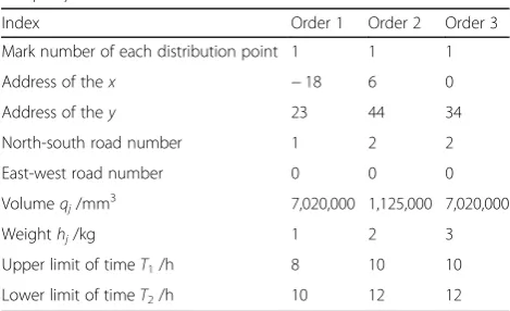
Table 3Information on delivery of cargo (part) (scale is 1:20,000)
Index Order 1 Order 2 Order 3
Mark number of each distribution point 1 1 1
Address of thex −18 6 0
Address of they 23 44 34
North-south road number 1 2 2
East-west road number 0 0 0
Volumeqj/mm3 7,020,000 1,125,000 7,020,000
Weighthj/kg 1 2 3
Upper limit of timeT1/h 8 10 10
number. If the shortest distance between two points passed through the third point, it was a number value of the third point. For example, path(i,j) =j meant i,j
points were directly connected along the road.
Path(i,j) =k meant the shortest distance between point
i and j should pass point k.
(2) Determine the driving path.
The pathrouterwas defined as ann×ncell array; rou-ter{i,j} represented the shortest path from pointi toj. If
iwas equal toj, router{i,i} = [i]. Ifiandjwere not equal, when path(i,j) =j, router{i,j} = [i,j] or when path(i,j) =k,
path(i,j) = [i, k, j].
Step 3: The number and specification of the truck were determined.
(1) Determine the truck quantity.
According to the load weight and volume of the truck, the order was from large to small. The mini-mum number of vehicles for kl was determined based on the weight and volume requirements of the deliv-ery cargoes.
(2) Determine the truck specification.
0-1 integer algorithm was used to determine the truck specification. The minimum rated capacity of all trucks was set as the target function.klis the upper limit of the
number of trucks, so as to ensure that the cargoes could be fully loaded as the constraint conditions.
2.3.3 Design of the distribution path algorithm based on the pickup cargo information
Step 1: Initial planning. In the case of only consider-ing the minimum distance, tabu search algorithm was used to calculate the optimal sequence based on the shortest distance matrix of all the cargo ad-dresses. Address information of cargo and distribu-tion center was randomly selected as the initial solution.The neighborhood search was made by pair-wise interchange. The round number of pffiffiffia (a was the sequence number) was set as the tabu length. 50a was set as the maximum iterations to calculate the optimized sequence.
Step2: Sequence division. th groups of sequences were randomly generated. The initial route S was di-vided into kl variety groups. t feasible solutions were found out based on the volume and weight of truck load capacity. Then, the least increase distance (the dis-tance between the distribution center and subsequence header + the distance between the distribution center and subsequence tail−the distance between two subse-quences) was made as the target to determine the opti-mal grouping situation, adjust the sequence order of optimal grouping, and form the initial solution which meets the service process.
Step 3: Optimize again. kl sequences were optimized with a minimum target function of time cost and transportation cost. The minimum cost was set as the target based on the time window and the rules of the pickup cargoes. The tabu search algorithm was used to re-adjust each sequence to obtain the optimal se-quence. The first element of the initial solution was distribution center, the others was the sequence got-ten from the second step. After the first element was fixed in the sequence, neighborhood search was made by pairwise interchange. Neighborhood space con-straints included two conditions. One was that when the free space of the truck was more than half of the truck load, the pickup cargo business started. The other was that before the delivery cargo business was completed, the pickup cargoes should not be more than half of the truck load.
Table 4Information on the collection of cargo (part) (scale is 1:20,000)
Index Order 1 Order 2 Order 3
Mark number of each distribution point 2 2 2
Address of thex −42 −6 −36
Address of they 8 24 8
North-south road number 0 2 0
East-west road number 8 0 8
Volumeqj/mm3 1,120,000 936,000 4,784,000
Weighthj/kg 2 2 1
Upper limit of timeT1/h 10 10 8
Lower limit of timeT2/h 12 12 10
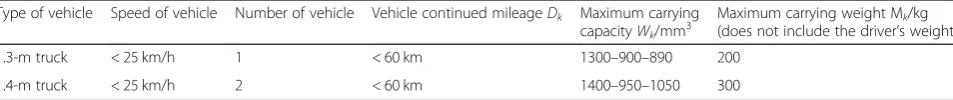
Table 5The vehicle information
Type of vehicle Speed of vehicle Number of vehicle Vehicle continued mileageDk Maximum carrying
capacityWk/mm3
Maximum carrying weight Mk/kg
(does not include the driver’s weight)
1.3-m truck < 25 km/h 1 < 60 km 1300–900–890 200
2.3.4 Inspection and display
Inspection included whether distance traveled was more than the rated distance traveled. If not, it was displayed that black lines were road routes, the yellow point was the distribution center, and the red line was the driving
route, or else the truck number was added once more and grouping planning was made again. If the truck did not meet the requirements, it indicated “the existing equipment cannot meet the requirements, please add new equipment.”
3 Experiment and discussion 3.1 The example design
Certain distribution sites provided services in Harbin. The delivery and pickup cargo information, road information, and truck information are shown in Tables 1, 2, 3, 4, and 5. The average transport cost per truck Cijk was 3.5 yuan/km. If it was not more than the service time range of 1 h before and after, x
was time delta/60 yuan (time is measured in mi-nutes), or else, x was 2 yuan (a1=a2= 1,c1=c2= 2). Road information is shown in Table 1 and Table 2. (The serial number was identification of this street/ road.) The information of the delivery and pickup cargo and their respective service requirements are shown in Table 3 and Table 4. (If the road number was 0, it indicated that it did not belong to the road.) The truck information is shown in Table 5.
3.2 Tabu search design based on MATLAB
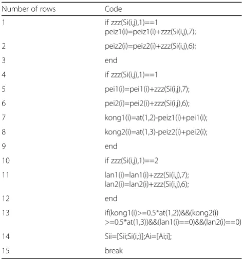
According to the initial planning, sequence planning, and re-optimization in the tabu search design, the design of MATLAB code editing was carried out. The main coding of the optimization was as follows.
Optimization was made again based on the third step in Section 3.3. When the free space of the truck was more than half of its load space, the pickup business started as shown in Table6.
Before delivery was finished, the volume of the pickup cargo could not be more than half of the truck space. The related programming was as follows:
(kong11(i)==at(1, 2))&&(kong22(i)==at(1, 3))&&(lan11(i)<=0.5*at(1, 2))&&(lan22(i)<=0.5*at(1, 3))
The klsequence is optimized with the minimum time cost and transportation cost as the target function as shown in Table7.
3.3 Experimental result display
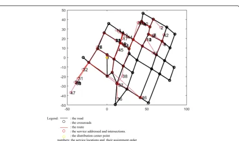
Figure2shows the road map of a“1.3-m truck.”Figure3 was a “1.4-m truck.” The black lines were road routes, and the yellow label was the distribution center point which was the starting point. In the graphics, all red cir-cles were the areas the service addressed and intersec-tions. The service places were marked by a number as their assignment order. The red line was the route. In Figs. 2 and3, part of the road numbers was shown. For example, the number of Tieshun Street was 1 and Tielu Street was 2. Figure 4 shows a change diagram of the distance calculation process in the initial planning
Table 6The code 1
Number of rows Code
1 if zzz(Si(i,j),1)==1
Number of rows Code
1 DistanV=0;n=size(s,2);
2 for i=1:(n-1)
3 DistanV=DistanV+20*dislist(s(1,i),s(1,i+1));
4 end
5 DistanV=DistanV+20*dislist(s(1,n),s(1,1));
6 P=[]; timecost(1,1)=0; P(1,1)=8;
Fig. 2Planning route 1. Black line represents the road, black circle represents the crossroads, red line represents the route, red circle represents the areas the service addressed and intersections, yellow circle represents the distribution center point, and numbers represent the service locations and their assignment order
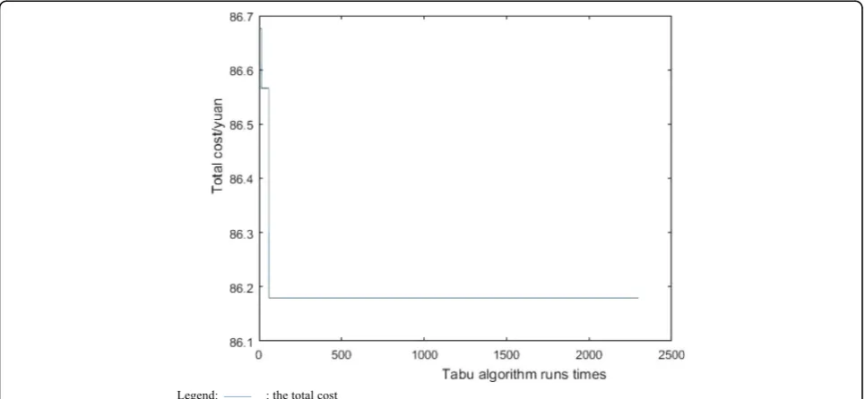
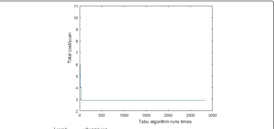
process. The total driving distance was observed from the initial 53 to 47.8 km, with the decrease of 9.81%. Fig-ures5 and 6 respectively show a change diagram of the cost of routes 1 and 2. The average cost reduced is about 8.76%. Two calculations were effective in reducing the cost of operation services and improving service levels. The whole truck scheduling algorithm combined cargo space and reasonable segmentation constraints into the distribution cargo route planning problem related to a
not full load. The algorithm included the road informa-tion processing to make the results intuitive and easy to operation.
4 Conclusion
The delivery and pickup cargo route plan math model was built based on time windows and load constraints. It was designed from the delivery order and path based on the Floyd Algorithm and road constraint. The 0-1 Fig. 4When the tabu search algorithm was firstly used. The sequence total operation distance variation diagram. The blue line represents the total operating distance
integer programming was used to determine the number and type of trucks, and then, the distribution routes and order algorithm were designed based on the tabu search algorithm under the influence of pickup cargo informa-tion. In a case, this method could divide the delivery ser-vices and pickup serser-vices reasonably, effectively solving the distribution route optimization problem under the influence of pickup cargo and various constraint condi-tions. According to the truck requirement and distribu-tion operadistribu-tion requirements, the method can be used selectively by different distribution practitioners.
Acknowledgements
The research presented in this paper was supported by Northeast Forestry University, China.
Funding
This study was supported by the Fundamental Research Funds for the Central Universities(No. 2572016CB13),the Postdoctoral program in Heilongjiang province(No LBH-Z2018).
Availability of data and materials
Not applicable.
Declarations
Not applicable.
Authors’contributions
All authors contribute to the concept, the design, and developments of the theory analysis and heuristic algorithm and the simulation results in this manuscript. All authors read and approved the final manuscript.
Competing interests
The authors declare that they have no competing interests.
Publisher’s Note
Springer Nature remains neutral with regard to jurisdictional claims in published maps and institutional affiliations.
Received: 14 May 2018 Accepted: 11 January 2019
References
1. M.Y. Zhai, J. Zhu, Study on current development status, problems and countermeasures of rookie network [J]. Logistics technology35(5), 63–67 (2016)
2. J. Zheng, Y.M. Cheng, Optimization design of the delivery route by vehicles scheduling program with time windows [J]. Logistics engineering and management32(10), 89–90 (2010)
3. W.G. Song, H.X. Zhang, L. Tong, C-W algorithm for vehicle routing problem of non-full loads with time windows [J]. Journal of Northeastern University
27(1), 65–68 (2006)
4. J.M. Li, Y.R. Ni, Y. Zheng, et al., Road network modeling and application oriented to third-party l ogistics distribution[J]. Computer integrated manufacturing system15(9), 1765–1769 (2009)
5. H.Y. Wen, Y.X. Shen, A method of computing weight of logistics navigation route planning based on analytic hierarchy process [J]. Journal of Highway and Transportation Research and Development25(8), 114–118 (2008) 6. B.Q. Ding, J. Jiang, Path optimization of logistics distribution vehicle based
on ant colony algorithm and dynamic road impedance [J]. Forest Engineering30(2), 149–152 (2014)
7. J. Li, Q.L. Da, R.Y. He, Pricing credit risk with multivariate stochastic volatility model[J]. Journal of Management Science in China13(10), 1–7+62 (2010) 8. J. Li, Y. Zhang, The study on vehicle routing problem of simultaneous
deliveries and pickups with time windows [J]. Inf. Control.38(6), 752–758 (2009)
9. J. Li, Y. Zhang, A tabu search algorithm for vehicle routing problem with simultaneous deliveries and pickups [J]. Theory and practice of system engineering27(6), 117–123 (2007)
10. K.R. Weng, K.J. Zhu, G. Liu, Collaborative transportation route optimization with lower bound flows [J]. Journal of system & management24(1), 38–42 (2015)
11. W.Q. Bie, Y.J. Li, Study on multiple vehicle routing problem integrated terminal cargo based on improved tabu search in distribution center[J]. Computer engineering and application46(4), 216–218 (2010) 12. Ç. Bülent, A new saving-based ant algorithm for the vehicle routing
problem with simultaneous pickup and delivery [J]. Expert Systems With Applications37(10), 6809–6817 (2010)
simultaneous pickup and delivery with time limit [J]. Eur. J. Oper. Res.
242(2), 369–382 (2015)
14. W. Yong, M. Xiaolei, X. Maozeng, L. Yong, Y. Wang, Two-echelon logistics distribution region partitioning problem based on a hybrid particle swarm optimization-genetic algorithm [J]. Expert Syst. Appl.42(12), 5019–5031 (2015)