Gaussian Sampling Precision in Lattice Cryptography

(1)

Gaussian Sampling Precision in Lattice Cryptography

Markku-Juhani O. Saarinen Centre for Secure Information Technologies (CSIT)

ECIT, Queen’s University Belfast, UK

Abstract

Security parameters and attack countermeasures for Lattice-based cryptosystems have not yet matured to the level that we now expect from RSA and Elliptic Curve imple-mentations. Many modern Ring-LWE and other lattice-based public key algorithms require high precision random sampling from the Discrete Gaussian distribution. The sampling procedure often represents the biggest implementation bottleneck due to its memory and computational requirements. We examine the stated requirements of pre-cision for Gaussian samplers, where statistical distance to the theoretical distribution is typically expected to be below2−90_or₂−128_{for 90 or 128 “bit” security level. We} argue that such precision is excessive and give precise theoretical arguments why half of the precision of the security parameter is almost always sufficient. This leads to faster and more compact implementations; almost halving implementation size in both hardware and software. We further propose new experimental parameters for practical Gaussian samplers for use in Lattice Cryptography.

Keywords: Post-Quantum Cryptography, Lattice Public Key Cryptography, Gaussian Sampling

1. Introduction

Most modern Ring-LWE and other lattice-based cryptographic algorithms require variables to be sampled from the Discrete Gaussian distribution. For many implemen-tations the sampling procedure represents the biggest performance bottleneck due to its memory or computational requirements. This is especially the case for embedded or lightweight targets such as smart cards [1, 2, 3, 4, 5].

Structure of this paper and our contributions. In Sections 2 and 3 we discuss the dis-crete Gaussian distribution, sampling, and precision. In Section 4 we argue that the common requirements for precision in Gaussian sampling are excessive; essentially only half of the bits are required, enabling faster and more compact implementations. We conclude with new, more efficient sampler parameters in Section 5.

(2)

.. -8 . -7 . -6 . -5 . -4 . -3 . -2 . -1 . 0 . 1 . 2 . 3 . 4 . 5 . 6 . 7 . 8 . _x .

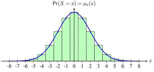
Pr(X=x) =ρσ(x)

Figure 1: The Discrete Gaussian distributionDσ (Equation 3) is defined for allx ∈ Zand satisfies ∑∞

x=−∞ρσ(x) = 1. The green discrete bars illustrate the probability mass and the blue line is the

corre-sponding continuous probability density function.

2. The Discrete Gaussian Distribution

For simplicity we use zero meanc = 0throughout this paper. Discrete Gaussian distributionsDσ are then defined solely by deviation parameterσ. The probabilities

forx∈Z(Figure 1) are proportional to

fσ(x) =e− x2

2σ2. (1)

We define a one-sided cumulative functionSσ(b)forb≥0asSσ(0) = 0,

Sσ(b) = b−1

∑

k=−b+1

fσ(k) f or b≥1. (2)

Due to symmetryfσ(x) =fσ(−x)we haveSσ(b) = 1 + 2 ∑b−1

k=1e−

k2

2σ2 _for_b≥_1. Since the limit for total scaling massSσ(∞)is very closely approximated byσ

√

2π

whenσgrows, we may use this scaling value in practical computations. LetP be a discrete random variable on sample spaceZ. The probability mass for anyx∈Zis

ρσ(x) =P r(P =x) =

fσ(x)

Sσ(∞)

≈e− x2

2σ2

σ√2π. (3)

(3)

Sampling Precision. LetP andQbe two discrete random variables on the same do-main. We use shorthandP(x) = Pr(P = x)andQ(x) = Pr(Q = x) for their distributions. Thetotal variation distanceδbetweenP andQis defined as:

ϵ=δ(P, Q) = 1

2||P−Q||1= 1 2

∑

x

|P(x)−Q(x)|. (4)

If we setP as the theoretical distribution (“perfect sampler”) and Qas the actually generated distribution, we may use the statistical distance between the two to quantify the quality of theQsampler.

Tail cutting. In tail cutting we ignore the “tail” portion of distribution with|x|> βσ

that has very small total mass, under target distanceϵ or related precision 2−λ. A typical tail cutting bound for cryptographic applications isβ = 13.2as it is easy to show that for anyσ≥1we have a negligible tail mass:

1−Sσ(13.2σ)

Sσ(∞)

<2−128. (5)

It is easy to see thatϵ <2−λ_βσ_where_βσ_{is the tail cutting bound.}

Required distance. It has been widely assumed that for cryptographic applications the sampling distance should be roughly the inverse of the security parameter [6]:

It is necessary for the rigorous security analysis that the statistical dif-ference between the actual distribution being sampled and the theoretical distribution (as used in the security proof) is negligible, say around2−90 to2−128.

This is also the precision typically now being implemented (See e.g. [7, 8, 9, 10]). In this paper we set out to show that such precision is essentially unnecessary sinceno algorithmwill be able to detect the difference from the non-tail portion of samples; only about half of this precision is actually required in almost all cases.

Other metrics and related work. Recently, proofs of some Lattice based schemes have been reworked using Rényi distance [11, 12] to require less precision in implemen-tations. Furthermore, Pöppelmann, Ducas, and Güneysu used the Kullback-Leibler divergence to reduce storage requirements in a hardware sampler implementation [10].

3. Approximate Sampling

Perfect sampler. First consider an arbitrary-precision sampler that converts an uni-formly random numberx∈R,0 ≤x <1into the Discrete Gaussian distribution by finding the “bin”i∈Z, i≥0in Cumulative Distribution Table (CDT) satisfying

Sσ(i)

Sσ(∞)≤

x < Sσ(i+ 1) Sσ(∞)

. (6)

(4)

Approximate sampler with precisionλ. We define an approximation where we use a

λ-bit uniform random integerj∈Z,0≤j <2λto approximate the discrete Gaussian Distribution. Here we again find the correct binivia

Sσ(i)

Sσ(∞) ≤

2−λj < Sσ(i+ 1) Sσ(∞)

. (7)

Now for a sampling error to occur at all,2−λjmust fit exactly on one of the thresh-old valuesi so thatλleftmost bits match with the cumulative distribution function:

2−λj≤ Sσ(i) Sσ(∞) ≤

2−λ(j+ 1). (8)

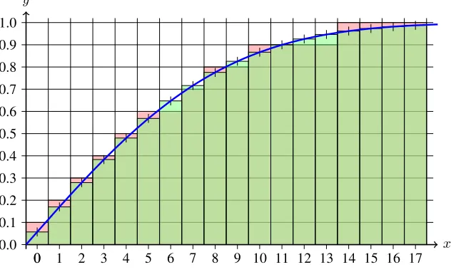
In practice, the probability of sampling error is almost directly proportional to sam-pling precision2−λ _{and total variation distance}_ϵ_{(Equation 4). See Figure 2 for an}

illustration of sampling error and the resulting statistical distance.

Binary Search in Cumulative Distribution Table. Since each half of the distribution function is monotonically decreasing (or increasing), we may perform a binary search on it in with at most⌈log2n⌉< λsteps, wherenis the number of entries in the table (integers with greater than “tail cutting” probability). This approach is widely used in real-life implementations [7, 10].

Other Gaussian Sampling Algorithms. High precision non-uniform continuous ran-dom sampling is a classic problem [13]. Many of the algorithms of the continuous case also apply to discrete cryptographic applications. Methods such as Inversion Sampling [14], Knuth-Yao Sampling [6, 15], The Ziggurat Method [1, 16, 17, 18], Kahn-Karney Sampling [19], and “Bernoulli” sampling [2] have also been proposed for lattice cryp-tography. For more (non-cryptographic) methods, see [20].

4. Distinguishing Distributions

When determining the appropriate sampling precisionλ, we are led to ask “What is the minimum statistical distance or precisionλthat can be detected by an adversary?”. If an approximation cannot be distinguished from true distribution with reasonable effort, there should not be any reason not to use it.

Tight bounds for distribution identity testing. We quote the following definitions and a recent result (Theorem 1 from [21, 22]) which offers very tight asymptotic bounds for the sample complexity of distribution identity testing:

Definition 1. For a distributionP, letP−max denote the vector of probabilities ob-tained by removing the entry corresponding to the element of largest probability.

Definition 2. For a vectorP andϵ > 0, defineP₋ϵ as the vector obtained from P

by iteratively removing the smallest domain elements and stopping before more thanϵ

(5)

.. 0.0 . 0.1 . 0.2 . 0.3 . 0.4 . 0.5 . 0.6 . 0.7 . 0.8 . 0.9 . 1.0 . 0 . 1 . 2 . 3 . 4 . 5 . 6 . 7 . 8 . 9 . 10 . 11 . 12 . 13 . 14 . 15 . 16 . 17 . 0 . _x . y

Figure 2: Sampling the discrete Gaussian distribution withσ = 7and sampling precision0.1. The curve corresponds to the discrete, mirrored, scaled, cumulative distribution function that approaches 1 asxgrows. This can be used to convert uniform random0≤y <1to the distribution; for example any0.6≤y <0.7 would correspond tox=±7. The red (rounded up) and green (rounded down) areas illustrate the statistical distanceϵbetween the ideal distribution and the approximation. Ally >0.9and|x| ≥14are “tail”.

We observe that Definition 1 corresponds to removing the distribution centre (c = 0) and Definition 2 corresponds to tail cutting (Section 2). Therefore these cases need to be handled specially.

Theorem 1 (Theorem 1 of [21, 22]). There exist constantsc1, c2such that for anyϵ > 0and any known distributionP, for any unknown distributionQon the same domain, our tester will distinguishP=Qfrom||P−Q||1≥ϵwith probability2/3when run on

a set of at leastc1

||P₋−_ϵ/max₁₆||2/3

ϵ2 samples and no tester can do this task with probability

at least2/3with a set of fewer thanc2||

P₋−_ϵmax||2/3

ϵ2 samples.

The tight Θ(||p||2/3

ϵ2

)

sample complexity of “Valiant-Valiant” (Theorem 1) not only implies bounds for traditional computational complexity, but also the minimum ora-cle query complexity of attack regardless of the computational model used. This is essentially an information theoretic bound.

On binary hypothesis testing and randomised rounding. Consider a table ofλ-precision approximationsT[0,1, . . . ,2λ₋_1]:

T[i] =

⌊

2λ Sσ(i)

Sσ(∞) ⌋

. (9)

(6)

essentially yield a case of binary hypothesis testing. If the table is held in RAM, it is possible to randomise it by adding +1 to each entry during initialisation with probability 1

2; here one comes up with the precise case of an unknown static distribution that has maximum total variation distanceϵ <2−λβσ.

In practice we define the precision2−λto have a few more bits of precision than corresponding ϵ; we are actually distinguishing a very large family of distributions from the true one. If an implementor still feels that this is a concern for some severely limitedλ, rounding can be further randomised. If the condition of Equation 8 holds and the given random integerjmatches all bits ofT[i], a randomised rounding sampler will output eitheriori+ 1, depending on an additional random bit.

The tail detector test and conjecture. We note that the potentially infinite tail spread of the Gaussian distribution makes theP₋ϵterm problematic. Indeed, with tail cut at

ϵlevel (tail mass ofϵ) one could simply test if any of the values of tail appear; such a “tail detector” test would have complexityO(1/ϵ). This problem is sidestepped by Theorem 1 and we and also ignore this special case in current work. We conjecture that lack of tail has only marginal effect on the entropy of random quantities and the security of the resulting cryptosystem.

Recursive application of Theorem 1 on the tail. An inverse-CDT type generator “knows” when it is supposed to generate values from the tail; in a straightforward implemen-tation theλ-bit random integerj is at the2λ₋₁_{maximum or close to it. One can}

apply Theorem 1 recursively on the tail by definingP′ as the tail portion of the main distribution, and adjustingϵ′accordingly.

Example 1. HereP′ = P \P₋ϵ/16 would be a natural choice. Corresponding

ad-justed precision would beϵ′ =ϵ2_/₁₆_{. First step of such a sampling algorithm is to test}

if uniformly randomjsatisfiesj ≥2λ₋_r_where_r_{is relatively small. If this is a case,} we randomise an anotherj′ and utilise a search algorithm on a table of tail values. Otherwise we proceed normally with the main table. Overall required precision will still beλbits but the two-step approach removes the problem of tail distinguishers. Naturally the condition makes constant-time implementation more difficult. Note that the secondary tail table will be invoked with very low probability; this part of the code and its tables are quite probablynever actually usedwith the parameters proposed in Section 5. This is why we conjecture that it is unnecessary.

Impact on sampling precision in private key operations. In a lattice public key al-gorithm (such as Ring-LWE based encryption or signature alal-gorithm), the bounds of Theorem 1 directly indicate (up to a constant factor) the number of times the private key oracle must be invoked beforeanyalgorithm,quantum or non-quantum, can de-termine whether the samples it uses were drawn from perfectly sampled distribution or from one with total variation distanceϵto it. SinceO(ϵ−2₎_{probes are necessarily} required, one can generally set the sampling precision toλ=s/2where2s_{is the target}

(7)

5. Conclusions and Experimental Parameters for Lattice Cryptography

From the theory of Statistical Identity Testing we know thatΘ(||p||2/3

ϵ2

)

samples are required to determine if a sampled distribution differs from an ideal one by total variation distanceϵ(and we ignore samples from the distribution “tail” of weightϵ). Therefore an appropriate selection for sampling precision is2−s2 wheresis the desired security level. We conjecture that theϵ tail has negligible effect on the entropy of secret quantities and the security of Lattice-based cryptosystems of interest, especially signature algorithms.

Based on our findings, we propose the following implementation parameters that allow standard, significantly more efficient data types to be used. Here we conserva-tively claim that the new parameters maintain the original security against all offline attacks if no more than2λ_{private key oracle queries are allowed for any given private}

key. This is a reasonable assumption as private key queries cannot be parallelised or performed without the consent of the holder of the private key. We further assume that ring polynomials are of relatively small degreen.

Security Precision Tailcut Possible data type

2100 λ= 50 |x|<8.1σ IEEE 754 floating point (double) 2128 λ= 64 |x|<9.2σ 64-bit fixed point (uint64_t) 2192 _λ_{= 96} _|_x_|_<₁₁_.₄_σ _{IEEE 754 quadruple-precision} 2256 _λ_{= 128} _|_x_|_<₁₃_.₂_σ _{128-bit unsigned integer type}

Example. BLISS-I [2, 10] withσ= 215.75and claimed 128-bit security can equiva-lently useλ= 64and a CDT table of sizen = 2048entries (9.5σ) in constant-time binary search. The total size of the CDT table is therefore 16kB in this case and 12 simple comparisons are required to produce each sample in constant time (if we ignore memory cache variation).

Acknowledgments

This work was funded by the European Union H2020 SAFEcrypto project (grant no. 644729). The author wishes to thank Máire O’Neill, Ilya Mironov, and Steven Galbraith for their helpful comments.

References

[1] J. Buchmann, D. Cabarcas, F. Göpfert, A. Hülsing, P. Weiden, Discrete ziggu-rat: A time-memory trade-off for sampling from a gaussian distribution over the integers, in: T. Lange, K. Lauter, P. Lison˘ek (Eds.), SAC 2013, Vol. 8282 of LNCS, Springer, 2014, pp. 402–417, extended version available as IACR ePrint 2014/510. doi:10.1007/978-3-662-43414-7_20.

(8)

[2] L. Ducas, A. Durmus, T. Lepoint, V. Lyubashevsky, Lattice signatures and bi-modal gaussians, in: R. Canetti, J. A. Garay (Eds.), CRYPTO 2013, Springer, 2013, pp. 40–56, extended version available as IACR ePrint 2013/383. doi: 10.1007/978-3-642-40041-4_3.

URLhttps://eprint.iacr.org/2013/383

[3] T. Güneysu, T. Oder, T. Pöppelmann, Beyond ECDSA and RSA: Lattice-based digital signatures on constrained devices, in: DAC ’14, ACM, 2014, pp. 1–6.

doi:10.1145/2593069.2593098.

[4] V. Lyubashevsky, Lattice signatures without trapdoors, in: D. Pointcheval, T. Jo-hansson (Eds.), EUROCRYPT 2012, Vol. 7237 of LNCS, Springer, 2012, pp. 738–755.doi:10.1007/978-3-642-29011-4_43.

[5] S. S. Roy, F. Vercauteren, I. Verbauwhede, High precision discrete gaus-sian sampling on FPGAs, in: T. Lange, K. Lauter, P. Lison˘ek (Eds.), SAC 2013, Vol. 8282 of LNCS, Springer, 2014, pp. 383–401. doi:10.1007/ 978-3-662-43414-7_19.

[6] N. C. Dwarakanath, S. D. Galbraith, Sampling from discrete gaussians for lattice-based cryptography on a constrained device, Applicable Algebra in Engineer-ing, Communication and Computing 25 (3) (2014) 159–180. doi:10.1007/ s00200-014-0218-3.

[7] J. W. Bos, C. Costello, M. Naehrig, D. Stebila, Post-quantum key exchange for the TLS protocol from the ring learning with errors problem, in: 2015 IEEE Symposium on Security and Privacy, SP 2015, San Jose, CA, USA, May 17-21, 2015, IEEE Computer Society, 2015, pp. 553–570, extended version available as IACR ePrint 2014/599. doi:10.1109/SP.2015.40.

[8] R. de Clercq, S. S. Roy, F. Vercauteren, I. Verbauwhede, Efficient software imple-mentation of Ring-LWE encryption, in: DATE 2015, IEEE, 2015, pp. 339–344.

doi:10.7873/DATE.2015.0378.

[9] Z. Liu, H. Seo, S. S. Roy, J. Großschädl, H. Kim, I. Verbauwhede, Efficient Ring-LWE encryption on 8-bit AVR processors, in: T. Güneysu, H. Handschuh (Eds.), CHES 2015, Vol. 9293 of LNCS, Springer, 2015, pp. 663–682.doi:10.1007/ 978-3-662-48324-4_33.

[10] T. Pöppelmann, L. Ducas, T. Güneysu, Enhanced lattice-based signatures on re-configurable hardware, in: L. Batina, M. Robshaw (Eds.), CHES 2014, Vol. 8731 of LNCS, Springer, 2014, pp. 353–370, extended version available as IACR ePrint 2014/254. doi:10.1007/978-3-662-44709-3_20.

[11] S. Bai, A. Langlois, T. Lepoint, D. Stehlé, R. Steinfeld, Improved security proofs in lattice-based cryptography: using the Rényi divergence rather than the statisti-cal distance, in: ASIACRYPT ’15 (To Appear), Springer, 2015.

(9)

[12] K. Takashima, A. Takayasu, Tighter security for efficient lattice cryptography via the Rényi divergence of optimized orders, in: M.-H. Au, A. Miyaji (Eds.), ProvSec 2014, Vol. 9451 of LNCS, Springer, 2015, pp. 412–431. doi:10. 1007/978-3-319-26059-4_23.

[13] J. F. Monahan, Accuracy in random number generation, Mathemat-ics of Computation 45 (172) (1985) 559–568. doi:10.1090/ S0025-5718-1985-0804945-X.

[14] C. Peikert, An efficient and parallel gaussian sampler for lattices, in: T. Rabin (Ed.), CRYPTO 2010, Vol. 6223 of LNCS, Springer, 2010, pp. 80–97. doi: 10.1007/978-3-642-14623-7_5.

[15] D. E. Knuth, A. C. Yao, The complexity of nonuniform random number gen-eration, in: J. F. Traub (Ed.), Algorithms and Complexity: New Directions and Recent Results, Academic Press, New York, 1976, pp. 357–428.

[16] H. Edrees, B. Cheung, M. Sandora, D. B. Nummey, D. Stefan, Hardware-optimized ziggurat algorithm for high-speed gaussian random number generators, in: T. P. Plaks (Ed.), ERSA 2009, CSREA Press, 2009, pp. 254–260.

URL http://sprocom.cooper.edu/sprocom2/pubs/ conference/ecsns2009ersa.pdf

[17] G. Marsaglia, W. W. Tsang, A fast, easily implemented method for sampling from decreasing or symmetric unimodal density functions, SIAM Journal on Scientific and Statistical Computing 5 (2) (1984) 349–359.doi:10.1137/0905026. [18] G. Marsaglia, W. W. Tsang, The ziggurat method for generating random

vari-ables, Journal of Statistical Software 5 (8) (2000) 1–7. URLhttp://www.jstatsoft.org/v05/i08

[19] C. F. F. Karney, Sampling exactly from the normal distribution, preprint arXiv:1303.6257, Version 2 (2014).

URLhttp://arxiv.org/abs/1303.6257

[20] D. B. Thomas, W. Luk, P. H. W. Leong, J. D. Villasenor, Gaussian random num-ber generators, ACM Computing Surveys 39 (4). doi:10.1145/1287620. 1287622.

[21] G. Valiant, P. Valiant, Instance-by-instance optimal identity testing, Electronic Colloquium on Computational Complexity (ECCC) 20 (2013) 111.

URLhttp://eccc.hpi-web.de/report/2013/111

[22] G. Valiant, P. Valiant, An automatic inequality prover and instance optimal identity testing, in: FOCS 2014, IEEE Computer Society, 2014, pp. 51–60, full version available as http://theory.stanford.edu/~valiant/ papers/instanceOptFull.pdf.doi:10.1109/FOCS.2014.14.