Western University Western University
Scholarship@Western
Scholarship@Western
Electronic Thesis and Dissertation Repository
6-20-2018 11:30 AM
Learning Regularization Weight for CRF Optimization
Learning Regularization Weight for CRF Optimization
Jiaxiao Wu
The University of Western Ontario
Supervisor Veksler, Olga
The University of Western Ontario Graduate Program in Computer Science
A thesis submitted in partial fulfillment of the requirements for the degree in Master of Science © Jiaxiao Wu 2018
Follow this and additional works at: https://ir.lib.uwo.ca/etd
Recommended Citation Recommended Citation
Wu, Jiaxiao, "Learning Regularization Weight for CRF Optimization" (2018). Electronic Thesis and Dissertation Repository. 5414.
https://ir.lib.uwo.ca/etd/5414
This Dissertation/Thesis is brought to you for free and open access by Scholarship@Western. It has been accepted for inclusion in Electronic Thesis and Dissertation Repository by an authorized administrator of
In recent years, convolutional neural networks (CNNs) are leading the way in many com-puter vision problems. Since the development of fully convolutional networks, CNNs have been widely employed for low-level pixel-labeling problems, and successfully pushed the per-formance to a new level. Although CNNs are able to extract highly discriminative features, they typically assign a class label to each image pixel individually. This leads to various spatial inconsistencies. Therefore, CNNs are commonly combined with graphical models, such as conditional random fields (CRFs), to impose spatial coherence. CRFs were invented precisely for the task of imposing spatial coherence among image pixels. The coherence regularization weight serves an important role of controlling the regularization strength in the CRF optimiza-tion, and has a great influence on the quality of the final result. Traditionally this weight value is set to a fixed number for all images.
In this thesis, we propose a novel approach to learn the coherence regularization weight for each individual image using a CNN, and then apply this per-image-learned weight in the CNN+CRF system. We first construct a dataset where the optimal regularization weight for the CRF optimization has been pre-computed for each image. We adopt convolutional regression networks with standard architecture for learning, and tailor the input according to our problem. We test the effectiveness of our approach on the task of salient object segmentation where a graph-cut based CRF optimizer can generate globally optimal solution. We show that consis-tent performance improvements can be achieved by using the regularization weight learned on per-image basis as opposed to a fixed regularization weight for all images in the dataset.
Keywords: parameter learning, regularization weight, convolutional neural network, graph cut optimization
Acknowledgements
I would like to thank my supervisor, Prof. Olga Veksler, for her encouragement and advice throughout my graduate study. She inspired me to solve computer vision problems using deep learning models. It has been a privilege to work with her and other members of the UWO vision group. I would also like to send my special thanks to David Szeto who has been an excellent idea generator and good company. Our constant discussions and arguments led to many interesting ideas. Last, I want to express my appreciation for my family and friends who encouraged and supported me unconditionally.
Abstract i
Acknowledgements ii
List of Figures v
List of Tables vii
1 Introduction 1
1.1 Image segmentation . . . 1
1.2 Visual saliency and salient object segmentation . . . 2
1.3 Convolutional neural network approach for salient object segmentation . . . 2
1.4 Challenges of spatial coherence and boundary precision . . . 3
1.5 Our approach . . . 5
1.6 Thesis outline . . . 6
2 Related work 7 2.1 Neural networks . . . 7
2.1.1 Traditional neural networks . . . 8
2.1.2 Depth vs breadth . . . 8
2.1.3 Activation functions . . . 9
Logistic function . . . 9
Hyperbolic tangent function . . . 9
ReLU . . . 11
2.1.4 Training process . . . 12
2.1.5 Optimizer . . . 12
Following the sign via RMSProp . . . 12
Momentum . . . 13
Adam . . . 14
2.1.6 Convolutional neural networks . . . 15
Convolutional layer . . . 15
Stride . . . 16
Padding . . . 16
2.1.7 Max Pooling . . . 17
2.1.8 Regularization . . . 17
Batch normalization . . . 18
Dropout . . . 19
Weight decay . . . 19
2.2 Segmentation as energy minimization . . . 19
2.2.1 Unary data term . . . 20
2.2.2 Binary smoothness term . . . 21
2.2.3 Optimization via Graph Cuts . . . 22
Graph construction . . . 23
The min-cut problem . . . 23
Submodularity . . . 24
2.3 Combining CRFs with CNNs . . . 24
2.4 Parameter learning for CRFs . . . 25
3 Learning coherence regularization weight for graph cuts using CNNs 26 3.1 CNN-CRF system . . . 27
3.2 Dataset construction . . . 28
3.2.1 Acquisition of the saliency probability measures . . . 28
3.2.2 Acquisition of the ground truth regularization weight . . . 30
3.3 Network architectures . . . 31
4 Experiments 34 4.1 Dataset . . . 34
4.2 Evaluation metrics . . . 35
4.3 Details of learning . . . 36
Weight initialization . . . 36
Learning rate decay . . . 37
Dropout regularization . . . 37
4.4 Results . . . 37
4.5 Effectiveness of learning . . . 38
4.5.1 Distribution similarities betweenλopt,λpred andλf ixed . . . 38
4.5.2 Extensive evaluation: performance on other datasets . . . 40
4.5.3 Demonstration of result examples . . . 41
4.6 Hyperparameter selection . . . 41
4.7 Runtime . . . 44
5 Conclusion and future work 46 5.1 Conclusion . . . 46
5.2 Future work . . . 47
5.2.1 Obtaining more accurate ground truth labels . . . 47
5.2.2 Exploring different types of network architectures . . . 47
5.2.3 Learning regularization weight in an end-to-end system . . . 47
Bibliography 49
Curriculum Vitae 54
1.1 Example of different types of segmentation. From left to right: the original image, a semantic segmentation where image pixels are clustered together if they belong to the same object class, the salient object segmentation where the visually distinguishable object is separated from the background. Images edited based on original images from Boykov. . . 1
1.2 Examples of salient fixation map and salient object segmentation. Left image from [27], right image from [39]. . . 2
2.1 A multi-layer perceptron (MLP) with one hidden layer. The input, hidden, and output layers have three, four and two neurons respectively. Image from [22]. . 8
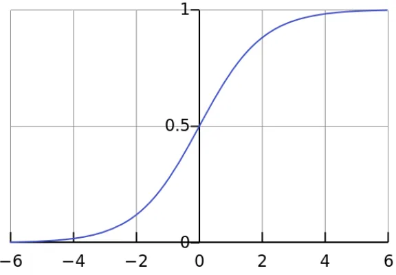
2.2 A plot of the (standard) logistic function. Image from Wikipedia, public domain. 10
2.3 A plot of the hyperbolic tangent (tanh) function. Image from Wikipedia, public domain. . . 10
2.4 A plot of the ReLU function (in blue). Image from Wikipedia, public domain. Discussion of the softplus function (in green) is beyond the scope of this work. . 11
2.5 Top: a visualization of a potential oscillation in the process of gradient descent. Bottom: a visualization of how momentum could smooth out the oscillation and help the algorithm descend more directly towards the local minimum. . . . 13
2.6 One-dimensional convolution examples with different stride values. The input is the lower layer of neurons and the feature map is the upper one. From left to right: convolution operation with stride 1; the same convolution, but with stride 2; the filter used to generate the feature maps. Image from [30]. . . 16
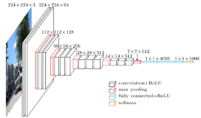
2.7 The architecture of the VGG-16 neural network. Note that the network uses a softmax function as output. Softmax function, also known as normalized exponential function, is often used in image classification tasks to represent a categorical distribution. Detailed discussion of softmax is beyond the scope of this work because we focus on training a regression network. Image from [19]. 18
2.8 The 4-neighborhood system. The pixels to the left, right, top, bottom of the pixelpare considered the neighbors of p. . . 20
2.9 A Graph Cut segmentation example. (a) input image, (b) segmentation with data term only, (c) segmentation with data term and smoothness regularization. Image from Y. Boykov. . . 21
2.10 Graph construction and Graph Cut segmentation. (a) shows all nodes in the graph. (b) and (c) demonstrate the graphical representations of the t-links and n-links in the graph. (d) shows a fully constructed graph. A cut is illustrated in (e) with the severed edges painted grey and a segmentation of the cut is shown in (e). Image from [48]. . . 22
3.1 Our CNN-CRF integration system. . . 27 3.2 The architecture of MS-FCN. Image from [39] . . . 29 3.3 The numbers of images assigned with each λopt label. The image samples
are from MSRA dataset of size 10K. The upper and lower limits of the λopt spectrum are 2−2and 217respectively. Theλoptlabel that fits the largest number of images is 128=27, which fits 1224 images. Theλ
opt label that fits the least number of images is 65536=216. . . . 30
3.4 The architectures of the two regression networks. . . 32
4.1 Image examples from MSRA10K dataset with their ground truth segmentation. 34 4.2 The histograms of the number of images preferring different regularization
weights. The horizontal axis lists out the bin values of regularization weights, and the vertical axis shows the image counts in the test set of the MSRA10K dataset. . . 39 4.3 Some successful examples. From left to right: original image, segmentation
produced by saliency-CNN, segmentation of CNN+CRF with the same regu-larization weightλf ixed for all images, segmentation of CNN+CRF with λpred learned by our weight-CNN, ground truth . . . 42 4.4 Some failure examples. From left to right: original image, saliency probability
map produced by saliency-CNN, segmentation of CNN+CRF with the same regularization weight λf ixed for all images, segmentation of CNN+CRF with λpred learned by our weight-CNN, ground truth . . . 43
4.1 F-measures of differentλacquisition methods evaluated on the MSRA10K test set and improvements relative toλf ixed . . . 37 4.2 The numerical similarity comparison of theλopt,λpredandλf ixedhistograms. . . 40 4.3 F-measures of differentλacquisition methods evaluated on the PASCAL dataset
and the improvements relative toλf ixed . . . 40 4.4 F-measures of differentλacquisition methods evaluated on the ECSSD dataset
and the improvements relative toλf ixed . . . 40 4.5 F-measures of differentλacquisition methods evaluated on the DUT-OMRON
dataset and the improvements relative toλf ixed . . . 41 4.6 Hyperparameter selection for Full-WCNN nets. Evaluation metrics are
com-puted on the validation set of MSRA10K across different values of initial learn-ing rate, number of neurons in the fully connected layers. The number of filters in convolutional layers are kept invariant as in VGG-16 nets. The parameters were selected based on MSLE loss. . . 44 4.7 Hyperparameter selection for Trimmed-WCNN nets. Evaluation metrics were
computed on the MSRA10K validation set across different values of initial learning rate, number of filters in the convolutional layers and number of neu-rons in the fully connected layers. The parameters were selected based on the MSLE loss. . . 45 4.8 The runtime, in seconds, required to compute the regularization weight using
Weight-CNN. . . 45
Chapter 1
Introduction
1.1
Image segmentation
The problem of image segmentation has been, and still is, a fundamental research topic in computer vision. Classical image segmentation is the process of partitioning a digital image into a set of regions that are visually distinct and homogeneous with respect to some charac-teristic or computed property, such as color, intensity, or texture. Image segmentation can also be formulated as a classification problem where each image pixel is assigned with one label from a set of pre-defined class labels [6, 51]. The resulting regions, or segments, consist of pixels with the same label. The criteria of the labeling encourage homogeneity between pixels of the same class and generally consider geometric information and chromatic characteristics. Image segmentation has many applications in various research fields, including medical image analysis such as exam result classification [57], tumour localization [47] and surgery planning [68]; object detection in satellite images [60] and thermal images [62]; and recognition tasks in video surveillance [71] and fingerprint identification system [53].
Given the ambiguity and the complexity of general purpose image segmentation, in this work, we instead focus on the most common type of segmentation: binary segmentation. This involves segmenting the object of interest from its background. In particular, we focus on segmenting the object with the property ofvisual saliency[3, 39].
Figure 1.1: Example of different types of segmentation. From left to right: the original im-age, a semantic segmentation where image pixels are clustered together if they belong to the same object class, the salient object segmentation where the visually distinguishable object is separated from the background. Images edited based on original images from Boykov.
(a) Salient fixation map (b) Salient object segmentation
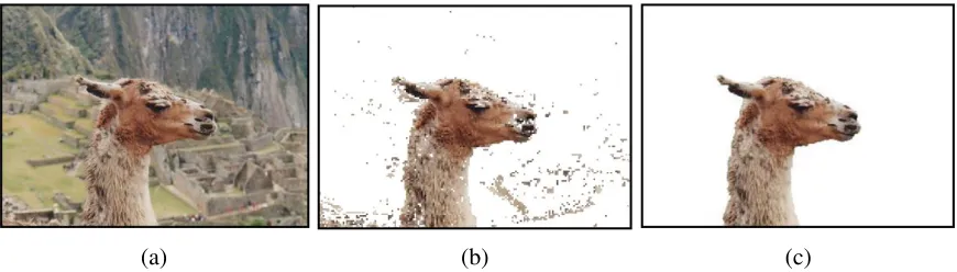
Figure 1.2: Examples of salient fixation map and salient object segmentation. Left image from [27], right image from [39].
1.2
Visual saliency and salient object segmentation
Visual attention is the ability of the human visual system to select only the salient visual stimuli for further processing. The saliency problem has been studied in various disciplines such as cognitive psychology, neuroscience, and computer vision. In computer vision, the pur-pose ofvisual saliency detectionis to identify the most visually distinct object in an image. The traditional approaches express saliency as human eye gaze when input images are displayed to human experimental subjects. Then the task of saliency detection is formulated as finding a saliency model that predicts the probability distribution of the location of the eye fixation over an image, i.e. thefixation map [8, 20, 27]. However, an increasing number of recent studies have found thatsalient object segmentation, which focuses on saliency prediction at the object level, is more useful in many computer vision and image processing problems, such as content-aware image resizing and photo visualization [42, 3, 39]. In Figure 1.2 (a) is an image with its fixation map, and an example of salient object segmentation result is provided in Figure 1.2 (b).
1.3
Convolutional neural network approach for salient
ob-ject segmentation
In recent years,convolutional neural networks(CNNs) have achieved remarkable successes in many computer vision tasks. Initially developed for image classification tasks, CNNs have expanded their influence into other high-level vision problems such as object detection, face recognition, and visual object tracking. Around 2015, Long, Shelhamer and Darrell [46] pro-posed the idea of thefully convolutional networkfor semantic segmentation. Since then, the usage of CNNs has been extended to pixel-labeling problems such as image segmentation, stereo correspondence, and optical flow [56, 72, 1, 15].
1.4. Challenges of spatial coherence and boundary precision 3
multi-context learning deep network that integrates both global and local contextual informa-tion to classify saliency for designated regions, and superpixels were used to ensure regional coherence.
Another category of CNN-based saliency models uses a fully convolutional architecture and end-to-end training [10, 39, 43, 66]. To our knowledge, one of the first multi-scale fully con-volutional networks that infer a pixel-level saliency map directly from the raw input image was proposed by Li and Yu [39] in 2016. This deep contrast model was paired with a segment-wise spatial pooling stream and a fully connected CRF to improve coherence. Almost simultane-ously, Liu and Han [43] presented a 2-stage end-to-end deep hierarchical model in which a coarse prediction map was produced in the first stage, followed by a hierarchical refinement network to recover image details progressively.
More recently, there were attempts to combine the task of salient object segmentation with other closely related vision tasks such as fixation prediction and semantic segmentation. A multi-task fully convolutional network was developed by Liet al. [41] to explore the intrin-sic correlations between saliency detection and semantic image segmentation. The proposed model collaboratively learns features for the two correlated tasks in the hope of improving object perception for saliency detection and reducing feature redundancy. Moreover, the idea of developing a unified network that is capable of solving multiple pixel-wise binary problems was explored by Houet al.[26]. With the observation that salient object segmentation, skeleton extraction and edge detection can all benefit from multi-level features in various degrees, Hou et al. proposed a horizontal cascade where highly abstract, deep representations are learned in the classic bottom-up structures and the multi-scale features are learned through the horizontal side pathsandtransition nodes.
Including but not limited to the above approaches, deep convolutional neural networks have achieved significant progress in salient object segmentation through the last two years. How-ever, regardless of their large capacity of representation, CNNs usually assign a label to each pixel individually, with no explicit enforcement of spatial coherence between the labeling of adjacent pixels. Therefore, there is still room for improvement over the generic CNN models that do not explicitly model this dependency of pixel labeling.
1.4
Challenges of spatial coherence and boundary precision
also reduce the resolution of feature maps. As a consequence, the loss of accuracy in spatial information is inevitable. The resolution loss in feature maps is even more influential for the more recent deep neural nets which tend to consist of more layers and more complex architec-tures. For image segmentation, losing resolution usually results in the loss of accuracy in the boundary area between salient object and background.
Problems of similar nature happen for other low-level vision tasks such as semantic segmen-tation, and relative impacts and current attempted solutions are reviewed in a survey [21].
Many new layers and structures were developed with the intention to preserve or restore spatial information to enhance the highly abstract features obtained from deep layers. The two common approaches are
1. combining outputs from different CNN layers by summation, concatenation or skip ar-chitectures [25]
2. modeling spatial relationships between nearby pixel labeling with some graphical models [16, 9]
Before CNNs are exploited to image segmentation, graph-based models including Markov Random Fields (MRFs) and Conditional Random Fields (CRFs) [37] were often used to encode relationships between pixels or superpixels based on hand-crafted features. With the expansion of CNNs, they are often incorporated in the CNN learning scheme as a post-processing step that models pixel label dependencies and improve spacial coherence.
When incorporating CRFs with CNNs, the probability measures learned by the CNN are often converted to the unary term in the CRF model, and some learned or fixed pairwise term is added to model the relationship between neighboring nodes. To control the regularization strength of the pairwise coherence term, it is a common practice to impose a weight factor, which, in this work, we refer to as regularization weightλ. With the weighted pairwise term, final segmentation result tends to be more spatially coherent, leading to an improved labeling accuracy.
In fact, the value of this regularization weight parameter λplays a key role in the spatial coherence of the final segmentation result. If λ is set too small, the length of the boundary between the object and background regions tends to be too long, resulting in over-segmentation. An over-segmented result consists of too many segments or the object boundary is not smooth enough. Ifλis set too large, the length of the object boundary tends to be too short, resulting in under-segmentation. In under-segmentation, the object boundary is too smooth and important shape details are omitted.
1.5. Our approach 5
1.5
Our approach
Even though a fixed value of the regularization weight λ is currently used for all images in CRF models, a better result might be achieved if each individual image can determine the amount of coherence regularization they need for themselves. This is because the appropriate amount of regularization required for a particular image can be influenced by multiple factors, including the image content, the edge contrast, and also on the quality of the unary term pro-duced by CNN for that particular image. If unary term is noisy, the weight parameter should be increased to make spatial coherence a stronger regularization. There are other non-obvious relationships between the best regularization weight and the image content and the CNN unary terms that one can attempt to learn.
Based on the above observations, in this work, we proposed to learn an appropriate value of the regularization weightλon a per-image basis. To learn the weight of coherence regulation, we exploited a convolutional network with a contemporary architecture, referred to as Weight-CNN. The input to weight-CNN is the color image, the unary probability measures used in the CNN-CRF system, and a tentative segmentation map based solely on the unary term. The output is used to predict an appropriate value for the regularization weightλwhich we then use during the CRF optimization using the graph cut algorithm [7].
Due to the novelty of learning the regularization weight in a supervised manner, we were not able to find any publicly accessible dataset for this problem. We constructed new datasets for training and testing based on the conventional saliency segmentation benchmarks. The examples in our augmented datasets consist of the color images coupled with their saliency probability measure maps and preliminary segmentation maps computed solely with unary saliency probabilities. The labels are the optimal regularization weight values estimated em-pirically from the ground truth saliency segmentations. We showed that, with our per-image-learned regularization weight, we can improve the F-measure metric of a CNN-CRF system in saliency segmentation.
The main contributions of this work can be summarized as following:
• We propose to learn the optimal weight of the coherence regularization on a per im-age basis for a CNN-CRF system. We employ a fully convolutional neural network to model the intrinsic relationship between the image content, the CNN-generated saliency probability measures and a good regularization weight. The proposed approach selects a regularization weight adapting to each specific input image, instead of a fixed weight for all images in the dataset, and achieves performance improvement in F-measure metric. It is worthy to mention that the proposed approach of regularization parameter learning can be extended beyond salient object segmentation, to any CRF-refined neural network training scheme.
F-measures achieved by the fixed regularization weights and the learned variable regu-larization weights. Consistent F-measure improvements observed on different datasets suggest the effectiveness of regularization weight learning.
• We present a procedure to augment the standard benchmark datasets of salient object segmentation with image-specific optimal coherence regularization weight that a CRF model can use to refine the CNN-generated segmentation results. Our experiment design and procedure might inspire further studies on other CRF parameter learning.
1.6
Thesis outline
Chapter 2
Related work
In this chapter, we review some fundamental architectures and techniques of convolutional neural networks that we employed for our regularization weight learning networks. We also discuss the conventional approach of modeling the image segmentation problem with CRFs and transferring the image segmentation problem into an energy minimization problem. Then, we review the graph cut algorithm, the optimizer in our energy minimization framework.
We are not aware of any prior work that applies deep learning to obtain the optimal regular-ization weight for CRF optimregular-ization in a supervised manner. However, there is prior work on combining CRFs with CNNs and prior work on parameter learning for CRFs, which we review in the latter two sections of this chapter.
2.1
Neural networks
Convolutional neural networks have led to major advances in computer vision in recent years [35]. In this section, we give an overview of the fundamentals of neural network design.
In general, neural networks are a machine learning model typically used to solve supervised learning problems such as regression or classification. They consist of an arrangement of multiple layers of artificial neurons, which loosely simulate the biological neurons of animals. The particular arrangement of layers depends on the type of neural network. This work only discusses multi-layer perceptrons and convolutional neural networks, but the topology of neural networks in common use is not limited to these two.
Within a given layer, each neuron takes an input vector and computes a linear function on it, giving an output scalar. The linear function is a set of weights learned as part of the training process for the neural network. The output scalar is typically then processed via a non-linear function known as anactivation functionin order to increase the expressive power of the neural network. A more detailed discussion on activation functions is given in Section 2.1.3. The particular arrangement of layers, the format of the input vectors, and the choice of activation function depend on the type of neural network being employed. In other words, they are hyperparameters of the general neural network model.
2.1.1
Traditional neural networks
Figure 2.1: A multi-layer perceptron (MLP) with one hidden layer. The input, hidden, and output layers have three, four and two neurons respectively. Image from [22].
A traditional neural network, also known as amulti-layer perceptron (MLP), consists of a sequence of layers of neurons. The output of the first layer is simply the input to the neural network. For example, in an image classification task, the image is the input. Within each layer after the first layer, the input vector to every neuron is the vector of outputs (after activation function) from the previous layer. We say that such layers are fully connected because every neuron in a given layer is connected to every neuron from the previous one. We call the intermediate layershidden layers.
The output of the overall neural network is simply the output of the last layer. Thus, the choice of the number of neurons in the final layer, as well as the final activation function, determine the format of the output of the neural network. For example, if the neural network is expected to output a probability, one would choose to employ a single neuron in the final layer and a logistic activation function in order to guarantee that the output will be between 0 and 1. Figure 2.1 shows a MLP with one hidden layer [30].
2.1.2
Depth vs breadth
2.1. Neural networks 9
edge performance on the ImageNet Large Scale Visual Recognition Challenge (ILSVRC) [59]. Then, in 2014, Simonyan and Zisserman [61] employed several networks with 16 to 19 learned layers to achieve newly-cutting edge performance in ISLVRC. The submission [23] to the 2015 iteration of the challenge employed networks up to 152 layers deep to earn 1st place.
Thus, in this work, we will treat increasing the depth of a neural network as being arguably synonymous with increasing its expressive power.
2.1.3
Activation functions
One employs non-linear activation functions in the intermediate layers of a neural network to increase its expressive power and the degree of potential non-linearity the network can com-pute. If one were to eschew activation functions, the resulting network would consist of a sequence of layers which computes a sequence of compositions of linear functions. However, from the associative property of matrix multiplication, one can derive the fact that a compo-sition of linear functions is itself a linear function. Linear models are simply not powerful enough to solve complicated vision problems. Therefore, a deeper neural network without activation functions would be no more powerful than a shallower one, all else being equal. Thus, employing activation functions in conjunction with increased depth allow a network to compute more abstract features. Here, we discuss the logistic, hyperbolic tangent, and ReLU activation functions.
Logistic function
Thelogistic function, also known as thesigmoid function, was a popular choice of activation function in the past. It is defined as:
σ(x)= L
1+e−k(x−x0), (2.1)
whereL,k, and x0 are constants affecting the behaviour of the function. Thestandardlogistic
function usesL= 1,k =1,x0 =0. In this work, all references to the logistic function will refer
to the standard logistic function. A plot of the function is available in Figure 2.2.
The output of the function, being bounded between 0 and 1, simulates a biological neuron either firing or not (or somewhere in between). Another common interpretation of its output, especially for the final layer, is that of a probability. This interpretation is convenient because probabilities also must be between 0 and 1.
Hyperbolic tangent function
Another formerly popular choice was thehyperbolic tangent function(tanh), defined as:
tanh(x)= e x−
e−x
ex+e−x. (2.2)
Figure 2.2: A plot of the (standard) logistic function. Image from Wikipedia, public domain.
2.1. Neural networks 11
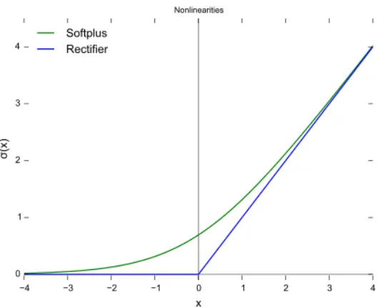
Figure 2.4: A plot of the ReLU function (in blue). Image from Wikipedia, public domain. Discussion of the softplus function (in green) is beyond the scope of this work.
except that its output is bounded between -1 and 1. Indeed, it can be seen that tanh is simply a shifted and re-scaled version of the logistic function:
tanh(x)= 2σ(2x)−1. (2.3)
For deeper networks, both the logistic and tanh functions suffer from thevanishing gradient problem. Because neural networks are typically trained with backpropagation, the rate of up-date for a given weight is proportional to the gradient of its activation function. However, both functions have a near-zero gradient for inputs with large absolute value. Thus, training can be-come excessively slow because of mini-scale per-iteration updates. This effect is magnified in deeper networks: a small update in the backpropagation process for a single layer will translate to small updates in earlier layers.
ReLU
TheRectified Linear Unit(ReLU) activation function [35] became a popular choice for deep networks because it doesn’t suffer from the aforementioned problem. It is defined as:
f(x)= x+= max(0,x). (2.4)
A plot of this function is available in Figure 2.4. It avoids the vanishing gradient problem because its gradient (for non-zero outputs) is always 1. It is also popular because both itself and its gradient are inexpensive to compute.
2.1.4
Training process
When employed in a supervised learning task, neural networks are typically trained using a process called backpropagation, an efficient implementation of gradient descent [30]. Back-propagation for a single training example works as follows.
1. The input training examplexis fed into the input layer of the neural network.
2. The neural network performs its computation layer-by-layer until its output yˆ is finally computed. We call this processfeeding forward.
3. The outputyˆ is compared to a label yusing aloss function, which computes a scalarC. For example, the squared error loss would computeC =P
i(yˆi− yi)2.
4. The weights of each layer are updated layer-by-layer in reverse order (hence the name backpropagation). The update rule for a single weightwiswt = wt−1−η∂w∂C
t−1 whereηis
thelearning rate hyperparameter. In this manner, the weight updates perform gradient descent on the costC.
The process described above constitutes gradient descent for a single training example. In prac-tice, neural networks are typically trained on mini-batches of training examples viastochastic gradient descent (SGD) or one of its variants [30]. Mini-batches are more convenient than training on single instances at a time because they are computationally efficient in practice on modern GPUs and they approximate the process of training on the entire dataset at a time bet-ter because the batches are randomly sampled from the overall set. At the same time, they are more convenient than the batch method (training on every instance simultaneously) because most modern datasets are too large to train on the entire batch at the same time. Also, normal-ization only updates the weights after processing the entire dataset, the learning is slower and less responsive to training samples.
2.1.5
Optimizer
As mentioned in Section 2.1.4, neural networks are typically trained using a variant of stochastic gradient descent. Modern optimizer additionally takes advantage of the ideas of momentumand following thesignof the gradient instead of both itssign and magnitude.
Following the sign via RMSProp
2.1. Neural networks 13
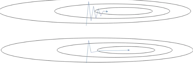
Figure 2.5: Top: a visualization of a potential oscillation in the process of gradient descent. Bottom: a visualization of how momentum could smooth out the oscillation and help the algo-rithm descend more directly towards the local minimum.
However, the Rprop algorithm was not designed with mini-batch-based training in mind. It assumes that the gradient is fixed, which is not the case for this kind of training. For example, the gradient of nine mini-batches may move a weight upwards by a value of 0.1, and then the tenth mini-batch may move the weight downwards by 0.9. The Rprop algorithm, assuming with a fixed step size of 1, would move this weight up by a value of 8 after the ten mini-batches, but clearly we would not want the weight to explode upwards like this. Or vice versa, weights could also explode downwards.
The RMSProp algorithm [64] attempts to fix this by dividing the weight update by the square root of a moving average of the squared gradient, instead of merely the magnitude of the current weight update as in Rprop. The exponential moving average of the squared gradient for a given weightwat time steptis calculated as follows:
MeanS quare(w,t)= decay×MeanS quare(w,t−1)+(1−decay)×(∂C ∂w(t))
2,
(2.5)
wheredecay is a hyperparameter denoting how slowly the old values of MeanS quaredecay exponentially. Tieleman and Hinton give a default value of 0.9.
Momentum
The strategy of gradient descent with momentum[52] attempts to reduce oscillation in the process of gradient descent (stochastic or otherwise). To borrow terms from physics, applying the momentum strategy treats the vector of the weights as a massive object with inertia and friction. Loosely speaking, the weight update process updates thevelocityinstead of the posi-tion of the object. Thus, it damps out oscillating forces over time. Figure 2.5 demonstrates the way momentum can change the path taken by a gradient in order to reduce oscillation.
More precisely, the weight updateVt at training step tcan be defined as an exponentially-weighted moving average of the previous updates:
Vt = βVt−1+(1−β)
∂C
where β is a decay hyperparameter affecting the proportion of the update coming from the previous momentum.
Adam
TheAdamoptimization strategy [31] is related to both RMSProp and SGD with momentum. Its name comes fromadaptive moment estimation.
In addition to keeping track of a moving average of the gradient for each weight, it keeps track of an exponentially-weighted moving average of thesquared gradient. The latter is used as an estimate of the un-centered variance of the gradient updates. During the weight updates, the average update is divided by the square root of this variance. As a result, if the variance of recent updates is high, the resulting update to the weight will be reduced.
The average gradient is calculated as follows:
mt =β1mt−1+(1−β1)
∂C ∂w ˆ
mt =mt/(1−β1),
(2.7)
wheremt is a biased estimate of the moving average, ˆmt is a biased-corrected estimate of the same,β1is an exponential decay hyperparameter,Cis the cost, andwis the weight in question.
Likewise, the average squared gradient is calculated as follows:
vt =β2vt−1+(1−β2)
∂C ∂w
!2
ˆ
vt =vt/(1−β2),
(2.8)
where vt is a biased estimate of the moving average, ˆvt is a biased-corrected estimate of the same, andβ2 is an exponential decay hyperparameter.
The overall weight update is as follows:
wt = wt−1−η
ˆ m √
ˆ
v+, (2.9)
where η is a learning rate hyperparameter and is a very small number included to avoid division by zero.
2.1. Neural networks 15
2.1.6
Convolutional neural networks
Convolutional Neural Networks(CNNs) have been applied to many problems in recent years [14]. CNNs employconvolutional layers in addition to the fully connected layers employed by traditional neural networks. Convolutional layers are simply layers which replace the lin-ear function with a convolution. The convolutional layers typically applin-ear before the fully connected layers. For example, the VGG-16 network [61] contains 13 convolutional layers (alongside some max pool layers, described in Section 2.1.7) followed by 3 fully connected layers.
Convolutional layer
The expressive power of a neural network is arguably bounded by the number of learnable weights it contains, which itself is bounded by the breadth and depth of the network. Fully connected layers contain many weights. In a fully connected layer withminput andnoutput neurons, there are mnweights. This can be computationally expensive to train and prone to overfitting, because even a single fully connected layer is so powerful.
As a more concrete example, suppose we want to analyze a 224 × 224× 3 image using a traditional MLP neural network. The input to the first fully connected layer would contain 224×224×3= 150528 neurons. If the output of the layer has the same dimensions, the number of trainable weights will be nearly 2.3×10¹⁰. Clearly, training even a single fully connected layer for a relatively small image is computationally prohibitive. Comparing to fully connected layers,convolutional layerstake advantages of spatial regularities in images in order to avoid employing an inordinate number of weights.
A convolutional layer extracts useful information and computesfeature mapsfrom an image or from feature maps computed by a previous layer by convolving a bunch of filters with learnable weights. Because the filter’s weights are learned, the layer can learn to perform simple tasks such as edge detection. Then, the extracted edges can be further processed in later convolutional layers for more complex tasks such as detection of parallelism. This can go on to be used in high level tasks such as detection of specific shapes. This process of solving low-level tasks in early layers and gradually progressing to higher-level tasks in later layers loosely reflects how the human visual system works, where early areas of the visual system solve lower level tasks and later areas focus on higher level ones.
A single feature map is computed as follows. Given an input of dimensionh×w×c, where h, w, and c stand for the height, width, and number of channels respectively, a n × n × c dimensional1filter is slid vertically and horizontally across the handwdimensions2. At each step in the sliding process, the weight associated with each cell in the filter is multiplied with the value it is currently positioned over in the input. These products are summed together
1It is possible for the filter to have different first and second dimensions, but in practice they are often the
same.
2This is the two-dimensional convolution. One- and three-dimensional versions exist; they simply require
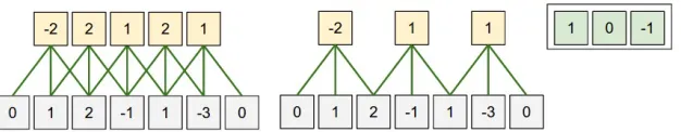
Figure 2.6: One-dimensional convolution examples with different stride values. The input is the lower layer of neurons and the feature map is the upper one. From left to right: convolution operation with stride 1; the same convolution, but with stride 2; the filter used to generate the feature maps. Image from [30].
to produce the value in the cell of the feature map at the given position. This operation is called aconvolution. In order to compute multiple feature maps from a given input, one simply performs the convolution multiple times using different filters.
Note that the third dimension of the filter is always the same as the number of channels from the input, so is typically omitted when stating the size. Thus, one would often say ”the filter has sizen×n”.
A major advantage of convolutional layers is the fact that they use fewer parameters because the parameters of each filter are shared to compute all cells in a feature map. This reduces training time and the chance that the neural network might overfit. At the same time, there is an intuition behind this kind of parameter sharing: if a feature is useful in one image location, it should be useful in all other locations. The convolution takes advantage of these regularities.
Stride
One can usestrideto generate a feature map significantly smaller than the input. Specifically, the stride is the number of pixels by which to translate the filter at every step of the convolution. A stride of 1 is the unaltered convolution described above. A stride of 2 slides the filter by two pixels every step in order to generate a feature map roughly half the size of the input in each dimension, and so on. See Figure 2.6 for a demonstration of how stride can reduce the size of a feature map.
In influential networks such as AlexNet [35] and the VGG nets [61], max pooling was used to reduce the size of successive feature maps rather than stride. These networks only used a stride of 1 in their convolutions. The neural networks in this work follow the same practice. See Section 2.1.7 for more information on max pooling.
Padding
2.1. Neural networks 17
have size (h−1)×(w−1). While there is nothing wrong with this, the most influential CNNs such as AlexNet [35] and VGG nets [61] have preferred to keep the feature map the same height and width as the input via the use ofzero padding. Other padding strategies have been used by other neural networks, but the discussion of them is beyond the scope of this work.
Zero padding implicitly extends the boundaries of the image with zero values. Suppose the filter size isnin the dimension of interest. The amount of zero padding required to keep the feature map the same size as the input would bebn
2c.
The neural networks in this work follow the strategy used by the aforementioned CNNs: zero padding is used before convolutions in order to make the feature maps have the same dimensions as their inputs.
2.1.7
Max Pooling
Apoolinglayer is used to reduce the dimensionality of the feature maps using some method to aggregate the responses. The AlexNet [35] and VGG nets [61] both usemaximum pooling (max pooling). Other pooling strategies exist, such as average pooling, but their discussion is not the focus of this work.
Max pooling aggregates responses of cells within a feature map by taking their maximum. Like convolutions, they use strides. A max pool with a 2× 2 filter and the stride of 2 will create a feature map by placing the filter on every other pixel positions and taking the max in the region covered by the filter. Thus, each dimension of the input will be halved. Likewise, the stride of 3 will take the max in the designated filter region placed on every 3 pixels, giving a feature map roughly one-third the size of the input in each dimension.
AlexNet and VGG nets use max pooling with stride 2 in order to halve the height and width of their feature maps. The neural networks in this work follow this strategy. The VGG nets use a total of five of these max pooling layers, giving feature maps 1/32 as high and wide as the original input images. See Figure 2.7 for a diagram of the architecture of the VGG-16 network.
2.1.8
Regularization
Figure 2.7: The architecture of the VGG-16 neural network. Note that the network uses a softmaxfunction as output. Softmax function, also known as normalized exponential function, is often used in image classification tasks to represent a categorical distribution. Detailed dis-cussion of softmax is beyond the scope of this work because we focus on training a regression network. Image from [19].
Batch normalization
Batch normalization[28] is a form of regularization applied to the output of a layer within a neural network. It can be applied to an image, a feature map (as output by a convolution or max pool), or simply a vector of data (as used by a fully connected layer). Batch normalization on the output of a given layer ensures that the data will have a consistent meanβand variance γ, which are learned parameters that change slowly over time. Thus, the next layer will receive data with a relatively consistent distribution, as a result, allowing a deep network to train with a higher learning rate while reducing fluctuations.
As its name suggests, batch normalization normalizes on a per-batch basis. A mini-batch is a subset of the training samples, often randomly selected; and the size of it is usually treated as a hyperparameter. As previously mentioned, neural networks are typically trained on mini-batches of its training dataset. Batch normalization ensures a relatively consistent mean and variance for each mini-batch.
Batch normalization applies to the following calculation to inputxin order to obtain output y:
y= √x−E[x]
Var[x]+ ×γ+β, (2.10)
2.2. Segmentation as energy minimization 19
the mini-batch means and variances collected at training time. represents a small number included in order to avoid division by zero.
Dropout
As previously mentioned, neural networks can contain hundreds of millions of learnable parameters. If a dataset doesn’t contain sufficient training examples, then many of these pa-rameters may not be properly trained before the neural network begins to overfit its training data. Thedropoutregularization strategy [63] attempts to encourage the neural network to train more of these parameters.
Like batch normalization, dropout is applied to the output of a neural network layer. It randomly zeroes out some of these elements with a probability p, where pis a hyperparam-eter. The elements which are zeroed out are then excluded from all feed-forward and back-propagation. The selected elements are chosen randomly on every forward call.
Dropout is employed only during the training process. It encourages the neural network to train using more parameters effectively, because different parameters will be zeroed out at different training steps.
Weight decay
Weight decayis an additional term added to the training loss in order to discourage any learn-able weight from growing too large. An unusually large weight is a symptom of overfitting, a problem where a model performs well on training data but does not generalize to unseen data. Thus, with weight decay, a weight will only grow large if necessary.
The modified lossLis calculated as follows:
L= L0+
1 2λ
X
i
w2i, (2.11)
where L0 is the original loss,wi represents theith weight in the network, and λis a hyperpa-rameter.
2.2
Segmentation as energy minimization
Figure 2.8: The 4-neighborhood system. The pixels to the left, right, top, bottom of the pixel pare considered the neighbors of p.
boundaries. Given the above notations, the problem of image segmentation can be expressed as an energy minimization problem [4, 6, 7] with the following energy
E(f)= X p∈Ω
Dp(fp)+λ
X
p,q∈N
Vpq(fp, fq), (2.12)
where Dp(fp) is a unary function that models the cost of assigning label fp to the pixel p, Vpq(fp, fq) is a binary function that penalizes label discontinuities,λis the weight factor bal-ancing the strength of coherence regularization, andNis a neighbouring system. In this thesis, we employ a 4-neighborhood system as demonstrated in Figure 2.8.
2.2.1
Unary data term
Dp(fp) is a function that measures how well pixel pfits label fp, and is often referred to as the data term. One of the most commonly adopted data terms is the negative log likelihood of the probability distribution for pixel pto have fpas the correct label [4, 51, 45]. The mathematical expression is
Dp(fp)=−logP(Ip | fp), (2.13)
whereIpusually represents some appearance information at pixelp, such as intensity or colour. When the log-likelihood function has a large value, the pixel pis more likely to be assigned with the label fp, and a small penalty should be applied to the energy function. The minus sign transfers the likelihood maximization task into a energy minimization problem.
For binary segmentation, the label set is L = {0,1}, and the data terms are calculated as follows:
Dp(0)=−logP(Ip |0) Dp(1)=−logP(Ip |1).
(2.14)
2.2. Segmentation as energy minimization 21
(a) (b) (c)
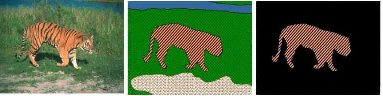
Figure 2.9: A Graph Cut segmentation example. (a) input image, (b) segmentation with data term only, (c) segmentation with data term and smoothness regularization. Image from Y. Boykov.
assignment of pixel pobtained solely by log likelihood test as in Equation (2.15) is not suffi -cient for a high quality segmentation.
fp =
0 if−logP(Ip |1)
P(Ip |0) > 0
1 otherwise (2.15)
Figure 2.9 demonstrates the case where appearance model alone is insufficient to distinguish object pixels from background pixels when some background pixels have similar colour fea-tures as the object pixels. The lack of spatial coherence results in a noisy segmentation in Figure 2.9 (b), and a prominent improvement was achieved in Figure 2.9 (c) by considering the label choices of surrounding pixels when assigning the label to a pixel.
2.2.2
Binary smoothness term
To encourage spatial coherence, a smoothness functionVpq(fp, fq) is employed to Equation (2.12), which introduces penalties when neighbouring pixels are assigned with different labels. This can be thought of as the cost of discontinuity in segmentation. Adding a smoothness term into the energy function encourages the segmentation results to have a shorter boundary. However, we also want to respect the observed data, so it is reasonable for the smoothness term to penalize more when the neighboring pixels with similar appearance features are assigned with different labels, but penalize less when neighboring pixels exhibiting distinct features are labeled differently. Thus, we adopt a widely used smoothness term [4, 51] in this thesis, which is defined as
Vpq(fp, fq)= wpq·I[fp , fq], (2.16)
where I[x]=
1 if condition xis true
0 otherwise (2.17)
and
wpq =exp(−
(Ip−Iq)2
Figure 2.10: Graph construction and Graph Cut segmentation. (a) shows all nodes in the graph. (b) and (c) demonstrate the graphical representations of the t-links and n-links in the graph. (d) shows a fully constructed graph. A cut is illustrated in (e) with the severed edges painted grey and a segmentation of the cut is shown in (e). Image from [48].
The cost weight function wpq describes the similarity in intensity between pixels p and q, namelywpq is large when pand qpossess similar chromatic features and close to zero when the adjacent pixels are very different.
2.2.3
Optimization via Graph Cuts
2.2. Segmentation as energy minimization 23
Graph construction
First, we establish the graphical representation of the energy minimization problem. Let G = {V,E} be a graph consisting of a set of nodes V and a set of undirected3 edges E. As
shown in Figure 2.10 (a), the node setV =V0∪ {s,t}consists of a node setV0where each node represents a image pixel and two special terminal nodes, thesource sand thesink t.
An undirected edge (p,q) is called a t-link or unary potential if p ∈ V0 and q ∈ {s,t}. As in Figure 2.10 (b), for every p∈ V0, both edges (p,s) and (p,t) ∈E. In the case of binary
segmentation, suppose the sourcesand the sinktrepresent the object label and the background label respectively, and then the edge weightwpsof the t-link (p,s) can be interpreted as the cost of assigning the pixel p to be the background. Similarly, the t-link (p,t) encodes the penalty for assigning pto be the object. Intuitively enough, the cost of assigning pixel pto one label should positively correlate to the possibility for pto take the alternative label. In computation, these costs are estimated by the data terms, and the positive correlations can be observed in Equation (2.19).
wps = Dp(t)=Dp(0)=−logP(Ip|0)= −log(P(Ip)−P(Ip|1))
wpt = Dp(s)=Dp(1)=−logP(Ip|1)= −log(P(Ip)−P(Ip|0))
(2.19)
An undirected edge (p,q) is called ann-linkorbinary potentialif p,q∈ V0. Between each pair of adjacent pixels, an n-link is added to E to encode the penalty of label discontinuity as shown in Figure 2.10 (c). The edge weights are calculated based on the similarity of pixel features as in Equation (2.18).
The min-cut problem
Ans-t cut,C= {S,T}, is a binary partition of graph nodesV, such that the source sand sink t are not in the same subset. That is, a cut separates the nodes inV into two disjoint subsets S andT, such that s ∈S, t ∈ T andV = S ∪T. The cutC can also be thought of as a set of edges, such thatCis a subset of the graph edge set Eand the edge setE−C does not contain any path from source terminal sto sink terminal t. The cost of a cut is defined as the sum of the weights of all severed edges, and the min-cut problem is to find the cut for a graph with the smallest cost. The green dash line in Figure 2.10 (e) demonstrates the min-cut on the given graph where the different thicknesses of the edge lines represent the values of the edge weights and the severed edges in the cut are painted grey.
A group of polynomial time algorithms that are widely adopted to solve the min-cut problem is based on the Ford-Fulkerson method [17]. The idea behind this method is to recursively find augmenting paths from the source to the sink, until no path with available capacity can be found anymore. Then the maximum flow from the source sto the sinktwas found, and the saturated edges divide the nodes into two disjoint subsetsS,T which is the cut with the minimum total
3Here, we construct an undirected graph because the employed edge weight function is commutative. One can
edge weight. Therefore, the max-flow and min-cut problems are equivalent, and the maximum flow passing from the source to the sink is equal to the total edge weight in the minimum cut4. For many vision applications where a graph model possesses the shape of two or high
dimensional grid, Boykov and Kolmogorov [5] developed a fast augmenting path algorithm of linear running time to realize the Ford-Fulkerson method.
Submodularity
The graph cut algorithm can only provide globally optimized result for certain classes of energy functions. Kolmogorov and Zabih [33] have proved that a pairwise energy with binary labels can be optimized by graph cut if and only if the energy satisfies the submodularity criterion. A pairwise energy function is considered to be submodular if it satisfies the following inequality
Vpq(0,0)+Vpq(1,1)≤Vpq(1,0)+Vpq(0,1) ∀p,q∈N. (2.20)
We can easily demonstrate that Equation (2.12) satisfies the above inequality using the defini-tion of the pairwise terms in Equadefini-tion (2.16).
Vpq(0,0)+Vpq(1,1)=0+0 Vpq(1,0)+Vpq(0,1)=wpq+wpq wpq≥ 0
∀p,q∈N
⇒ Vpq(0,0)+Vpq(1,1)≤ Vpq(1,0)+Vpq(0,1) ∀p,q∈N
(2.21)
2.3
Combining CRFs with CNNs
Convolutional neural networks are often used to estimate the possibilities for a pixel to take on different labels and assign the label with the highest possibility to each pixel individually. Even though the overlaps of the receptive fields have the potential of encoding some connection between nearby pixels, the label dependencies are not explicitly modeled by CNNs. To fill this insufficiency, CRFs are often employed to refine the CNN-generated results either as a post-processing step [16, 9] or as a part of a trainable system [76].
The earliest and most intuitive approach to incorporate CRFs is to use them as a post-processing labeling strategy. The typical method is to construct a CRF energy function with the label assignment probability learned by a CNN as the unary term and a pairwise term based on appearance to enforce local consistency, and then this energy is minimized by some optimiza-tion algorithms, such as [5, 7, 34]. As early as in 2013, Farabetet al. [16] paired a multi-scaled CNNs with the CRF refinement as one of their proposed labeling strategies for scene labeling, and managed to produce more visually satisfying results than no refinement and superpixel refinement. Chenet al. [9] used a fully connected CRF to model the pixel dependency after obtaining the pixel-wise label probabilities for semantic segmentation, and the pairwise poten-tials were calculated using Gaussian kernels in different feature spaces, i.e, the RGB colour
4This is known as the max-flow min-cut theorem, and was proven by multiple individual work [17, 13] in
2.4. Parameter learning forCRFs 25
and the pixel positions. An approximate inference of the CRF was computed using the mean field approximation [34]. The same fully connected CRF system was also employed for salient object segmentation problem [39, 25] to improve spatial coherence.
Another way to integrate CRFs with CNNs is to include the CRF optimizer into the end-to-end training scheme of the neural networks. Zheng and Jayasumana [76] formulated the mean field inference [32] of the CRFs with Gaussian pairwise potentials as recurrent neural networks. However, the performance of this method is limited by the mean field approximation, whose effectiveness was shown to be arguably questionable [67].
2.4
Parameter learning for CRFs
Before CNNs are widely applied to image segmentation, probabilistic graphic models, in-cluding CRFs and Markov Random Fields (MRFs), are commonly used for modeling the con-nections among nodes which correspond to pixels or super-pixels in images. Here we summa-rize some popular approaches for CRF parameter learning.
One approach to CRF parameter learning is to use the classical method of maximum like-lihood estimation [36]. In the context of CRFs, however, maximum likelike-lihood estimation is often intractable due to the presence of the joint conditional distributions. So, various approx-imations, such as pseudo-likelihood [40], are used instead. When applying, many statistical assumptions are made about the underlying data by the approximation algorithm, which might over simplify the problem and influence the quality of the estimation.
Zhang and Seitz [74] formulated the stereo correspondence problem as a maximum a poste-rior (MAP) problem in which both a disparity map and CRF parameters were estimated from the stereo pair itself. More precisely, they learned CRF parameters using statistical estimation based on the expectation maximization (EM) algorithm. Their approach learned parameters on a per-image basis, but it was computationally intensive, as the proposed EM procedure had to be run for multiple iterations for estimation and the stereo algorithm was required to be executed at least once in each iteration.
Learning coherence regularization weight
for graph cuts using CNNs
Convolutional neural network has led the way in many pixel-wise labeling problems of vi-sion, including salient object segmentation, semantic segmentation and scene understanding [56, 72, 1]. Essential to the success of CNNs is their ability to learn more abstract data rep-resentations and extract more compact features from images than traditional hand-crafted fea-tures [73]. However, when applied to dense prediction tasks, deep CNNs usually suffer from loosing spatial information with the loss of feature map resolution, which might result in the reduction of localized accuracy. For segmentation problems, this accuracy reduction mainly occurs in the boundary regions where more structural details are presented along with more noise.
As discussed in Section 2.3, a common approach to recover boundary accuracy in segmen-tation problems is to explicitly represent pixel dependencies with some graphical models, such as CRFs, and encourage spatial coherence. This involves formulating an energy function where the desired properties are encoded into one or several energy terms. Then the energy function is optimized and the labeling corresponding to its minimum gives the final segmentation.
Unlike in some previous work [39, 25] where fully connected CRFs were built and opti-mized using the mean field inference, we propose to build a CNN-CRF system where the CRF graph can be optimized by the graph cut algorithm as described in Section 2.2. A wide class of binary energy functions can be optimized by the graph cut algorithm [33]. For binary prob-lems where pixels can take on one of the two possible labels, graph cuts yield an exact, globally optimal solution; while graph cuts cannot solve exactly themulti-labelproblems where pixels can be assigned with more than two distinct labels, but the produced approximation are usu-ally near the global optimum [7]. The energy function we need to optimize for binary image segmentation belongs to the class of problems that can be optimized exactly [33]. Therefore, our proposed system benefits from the optimal solution generated by graph cuts, whereas the mean field inference used in [39, 25] is not a very effective optimization algorithm [67].
3.1. CNN-CRFsystem 27
Figure 3.1: Our CNN-CRF integration system.
An important but open problem in graph cut segmentation is parameter selection. Different choices of parameter values might result in large differences in the performance of the seg-mentation result. The standard approach is to select a fixed value for these parameters when running the graph cut segmentation algorithm on an entire dataset. This fixed value is set by hand, learned from the training data, or a combination of both. However, a segmentation with better visual performance can be expected if the regularization weight of coherence is chosen adaptive to each specific image.
This work investigate the possibility of using a CNN to choose an appropriate parameter value on a per-image basis; the focus of this work is on the selection of the regularization weightλfor the graph cut algorithm in the context of salient segmentation problems.
3.1
CNN-CRF system
3.2
Dataset construction
To solve the problem of learning an appropriate value for the regularization weightλ, one first needs to obtain a dataset from which a learning model can be trained on. Due to the novelty of the problem, we can not find any benchmark dataset and have to construct one for this new task. We start with a standard salient object segmentation dataset, which contains RGB images and the ground truth segmentations of typically one salient object labeled by hands. We augment these salient benchmark datasets to include more components.
The two critical components in our augmentation are a saliency measure map that evaluates the probability of assigning a pixel as foreground object, and the desiredλvalues with respect to the above saliency measure. The desired λvalues serve as the output labels in our dataset and are referred to as λopt in this thesis. The calculation of the saliency measure is important because the quality of the probability map directly influence the desired λvalues. The more accurate the probability map is, the less coherence information should be considered by a segmentation algorithm and the smaller the optimal λ value tends to be. In an ideal case, if we could obtain pixel-wise probability maps perfectly distinguishing the object from the background, we would not need to consider coherence between neighboring pixels and setλ value to be 0. However, in real applications, it is almost impossible to consistently obtain perfect saliency measure and a segmentation algorithm needs to consider blob coherence and boundary smoothness. Also, the saliency probability measures provide the data term in the energy function of graph cut image segmentation.
3.2.1
Acquisition of the saliency probability measures
As mentioned in the previous section, the network for saliency prediction in our CNN-CRF system, Saliency-CNN, can be substituted by any CNNs trained to give dense saliency probability measures. With the increased use of CNNs in various computer vision prob-lems, many CNN architectures have been proposed specifically for salient object segmentation [29, 75, 65, 38, 39] and have achieved competitive performances in different saliency bench-marks. We chose to adopt a VGG-16 based multi-scale fully convolutional network (MS-FCN) to obtain the saliency probability measures after examining different network architectures based on criteria, such as the rationality and effectiveness of structures, performance, repro-ducibility.
3.2. Dataset construction 29
Figure 3.3: The numbers of images assigned with eachλopt label. The image samples are from MSRA dataset of size 10K. The upper and lower limits of the λopt spectrum are 2−2 and 217 respectively. Theλopt label that fits the largest number of images is 128=27, which fits 1224 images. Theλoptlabel that fits the least number of images is 65536=216.
3.2.2
Acquisition of the ground truth regularization weight
The value of λ controls the smoothness of the segmentation boundaries, i.e., how many details and noises will be included in the segmentation boundary. An appropriateλvalue en-courages boundary smoothness and suppresses noises caused by inaccurate saliency probability measure. However, if λis set to be too big, the details on the object boundary might be lost. On the contrary, if theλvalue is set to be too small, too many noises will be captured, which leads to over-segmented result.
3.3. Network architectures 31
We choose the lower and upper limits of the spectrum empirically: we determine thatλopt rarely drops below 2−2 and rarely rises above 217. We decide that the interval between each
value ofλin our spectrum should grow exponentially because therelativeerror seems to affect our results more thanabsoluteerror. For example, the difference betweenλ = 10 vs λ = 11 was observed to matter far more than that ofλ= 10000 vsλ= 10001. The distribution of the calculatedλoptvalues of segmentation dataset MSRA10K [44] is shown in Figure 3.3.
3.3
Network architectures
We exploit two regression network architectures for learning the regularization parameterλ in the CRF energy function on a per-image basis. Both networks are alterations of the Ox-ford VGG-16 classification nets [61]. We adopt the main characteristics of VGG-16 network structure because VGG-16 and its variations have achieved remarkable performance in various vision tasks other than object classification which VGG-16 was developed for. Their recent success in semantic segmentation [46, 49] demonstrated the expressive power and the potential of VGG-16 structure to learn for other vision tasks.
We modify the VGG-16 net to our Weight-CNN by reducing the number of neurons in the output layer from the number of classes (for classification purpose) to one which outputs a real scalar value serving as the exponent of the predicted regularization weight value. We take the number of neurons in the fully connected layers as a hyperparameter to tune during training. We preserve the 5 max pooling layers with stride 2 in the original VGG-16 net. This is to reduce the feature map resolution in the hope of extracting more compact, positional invariant feature representations. Each convolutional layer has 3 × 3 kernels with stride 1, and the number of kernels grows exponentially between each convolutional group as in the VGG nets. Zero padding is employed before every convolutional layers for easy calculation of dimension changes.
One major difference between our two networks is the number of convolutional layers before each pooling layer. As shown in Figure 3.4 (a), the full Weight-CNN network (Full-WCNN) has 2 to 3 convolutional layers in each stage. A stage is a group of network structures that consist of one or more convolutional layers, batch normalization layers, ReLU activation lay-ers, and followed by a max pooling layer. For the trimmed Weight-CNN network (Trimmed-WCNN) in Figure 3.4 (b), there is only 1 convolutional layer in each stage. Additionally, in Full-WCNN, the two fully connected layers have the same number of neurons; meanwhile, in Trimmed-WCNN, the second fully connected layer has half as many neurons as in the first fully connected layer.
(a) Full-WCNN (b) Trimmed-WCNN
3.3. Network architectures 33
Based on empirical experiments, we decide to include 5 input channels for Weight-CNN including the RGB channels of an image, the saliency probability map and a tentative segmen-tation obtained by segmenting the saliency probability map using a 0.5 threshold. The output of Weight-CNN is a real scalar value, which serves as the exponent of the predicted regulariza-tion weight. Let ˆydenote the raw network output, then theλvalue that should be used as the regularization weight for graph cut algorithm is
λpred =2ˆ y.
(3.1)
The networks are trained to minimize the mean squared logarithmic error (MSLE) and aL2
weight decay term. Let L denote the ground truth label of λopt selected from a spectrum of exponential growth, let ˆy denote the raw network output, then, for a training batch of size n, the MSLE loss function can be expressed as
LMS LE = 1 n
n
X
i=1
(log(Li)−yˆi)2. (3.2)
Experiments
4.1
Dataset
MSRA10K is a popular salient segmentation dataset introduced by Cheng and Borji et al [11, 12, 2], and it proposed a solution to the problem that traditional salient object datasets with bounding box annotations only provide coarse evaluations for the salient segmentation al-gorithms. In the contrast, MSRA10K provides pixel-level saliency labeling for 10,000 images from MSRA Salient Object Dataset [44].
We choose MSRA10K for our experiments because of its large size. By the time our exper-iments were conducted, MSRA10K was the largest publicly accessible salient segmentation dataset. MSRA10K consists of a variety of images, including challenging samples shown in Figure 4.1 (b) where the boundary is richly detailed, Figure 4.1 (c) where the pixels of the salient object have colors similar to the background pixels colors, and Figure 4.1 (e) where the boundary between the salient object and the background is weak. The richness of the dataset is also helpful to reduce the potential overfitting when we experiment with different network structures.
(a) (b) (c) (d) (e) (f)
Figure 4.1: Image examples from MSRA10K dataset with their ground truth segmentation.
![Figure 1.2: Examples of salient fixation map and salient object segmentation. Left image from[27], right image from [39].](https://thumb-us.123doks.com/thumbv2/123dok_us/1946392.1256081/10.612.111.486.72.143/figure-examples-salient-xation-salient-object-segmentation-left.webp)