Direct simulation of the fluid-structure interaction of a compliant panel in a hypersonic compression ramp flow

(1)

c

(2)

DIRECT SIMULATION OF THE FLUID-STRUCTURE INTERACTION OF A COMPLIANT PANEL IN A HYPERSONIC COMPRESSION RAMP FLOW

BY

BRYSON SULLIVAN

THESIS

Submitted in partial fulfillment of the requirements for the degree of Master of Science in Aerospace Engineering

in the Graduate College of the

University of Illinois at Urbana-Champaign, 2019

Urbana, Illinois

Advisor:

(3)

Abstract

Sustained flight at hypersonic speeds presents a challenge to robust vehicle design and control. An extreme aerothermal environment acting on geometrically-thin, multifunctional structures can result in significant static and dynamic structural deformations of the vehicle and its subcomponents. In particular, for a control surface-motivated scenario, the adverse pressure gradient generated by a compression ramp can produce a large region of subsonic, separated flow with the potential to degrade accurate estimation of surface loading by traditional hypersonic aerodynamic methods such as piston theory. The present work details high-fidelity, coupled fluid-thermal-structure interaction (FTSI) simulations of laminar, unsteady 2D flow at M∞= 6.04 over a 35-degree compression ramp with an embedded

compliant panel. Surface-pressure loading generated by the corner shock wave boundary layer Interaction (SWBLI) is compared between compliant and non-compliant compression ramp configurations, and SWBLI-excited response of the compliant panel is demonstrated. An analytical model based on Rayleigh’s method is introduced which, given the maximum amplitude of vibration, predicts the nonlinear frequency of a compliant panel to within an average error of 8.3% over several orders of magnitude in flexural rigidity. Maximum observed heat transfer rates to the panel were diminished for the compliant panel cases relative to the rigid case, believed to be caused by a break-up in structure of the oscillating shear layer due to the motion of the panel. Reduced-order models, such as shock expansion/ local piston theory (SE/LPT), are computed for each panel and were found to perform well with a modification to account the influence of the corner separation region. Reynolds’ analogy for estimating heat flux was found to work reasonably well for the rigid case, but lost accuracy when applied to the thinnest panels and largest deflections.

(4)

(5)

Acknowledgments

In my life there have been countless people I’ve met—both personally and professionally— who have been instrumental in shaping the individual that I am today. It would be genuinely impossible to do them all justice in the limited space given here, but I will try my best. I must begin with a monumental thank you to each and every member of my immediate and extended family: Jackie, John, Dawn, Diara, T Kim, Frank, Sheila, Jordan, (and yes Jalen and Aiden) for being so incredibly supportive of me and my endeavors over the years. You remind me exactly why I do what I do, and give me the perspective to truly appreciate it. I love each and every one of you, the world is better for your being in it.

Special thanks must also be given to the academic and industry figures who in their own way have defined who I am as a professional and guided my passion for aviation and engineering: Stephen Ettorre, Scott Carson and Dave Halstead from GE Aviation Evendale, Shadie Tanious at CEi Kratos, Professors Carl Wassgren and Suresh Garimella at Purdue University, and Professor Jeffrey Bons at The Ohio State University. At the University of Illinois, special thanks must be given to Professors Micheal Selig, Phillip Ansell, Maciej Balajewicz, Paul Fischer, and Marco Panesi for your excellent instruction, many enlightening conversations, and the problems you’ve helped me solve in my time here. Finally, a special and extended thank you must be given to Professor Daniel J. Bodony, who has given me (and continues to give me) the opportunity to demonstrate my ability, grow as a technical professional, and contribute to an absolutely stellar research group.

I am especially thankful for the contributions of Wentao Zhang, Pooya Movahed, and Shreyas Bidadi, without whom the present analysis would not be possible. Recognition must also be given to my outstanding group members Cory Mikida, Fabian Dettenrieder, Mohammad Mehrabadi, Sandeep Murthy, Alex Fikl, Yong Yi Bay, Palash Shashittal, Shakti Saurabh, Mahesh Natarajan, Michael Banks and David Fellows, who have all (at one point or another) helped jump-start my brain, solve a problem, or just plain made things more fun. You are all legends, best of luck in your future endeavors.

Finally, I must give a tremendous and personal thank you to one Christopher Ostoich, whose persistent and timely input to this project cannot be overstated. Chris, you routinely took time you took out of your busy schedule to answer very technical questions with limited information, and this was never taken for granted or went unnoticed. Thank you so very much for your help along this journey, not all heroes wear capes!

(6)

List of Tables

2.1 Piston Theory Coefficients (m=√M2₋_{1) . . . .} ₂₄

3.1 RWTH-Aachen Freestream Conditions . . . 26

3.2 NASA-UMD Freestream Conditions . . . 30

3.3 NASA-UMD Model Geometry . . . 30

3.4 Fluid and Solid Grid Properties . . . 31

4.1 Eigenvalues of the Clamped-Clamped Euler-Bernoulli Beam . . . 45

4.2 Non-linear Frequency Ratios for a Clamped-Clamped Beam . . . 55

5.1 NASA-UMD Case Material Properties . . . 59

5.2 Parameters for FSI Cases (L= 3.475”) . . . 60

5.3 Fluid and Solid Grid Properties . . . 61

5.4 Nonlinear Vibration Frequency Comparison . . . 68

(9)

List of Figures

1.1 Artist Rendering of the X-43B Hypersonic Aircraft, NASA [3] . . . 1

1.2 North American X-15A-2 Hypersonic Research Aircraft . . . 2

1.3 Schematic of a hypersonic compression ramp configuration, Carter (1972) [9] 3 1.4 Surface pressure coefficient during LCOM∞= 1.2, Re= 1×105, Gordnier and Visbal (2003) [24] . . . 6

2.1 Interface Conditions for Fluid-Thermal-Structural Solver . . . 20

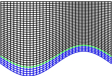
2.2 Qualitative illustration of conforming fluid grid (black), solid domain grid (blue), and interacting boundary (green) using TFI . . . 21

3.1 RWTH-Aachen Case: M∞= 7.7,ReL= 4.368×105 . . . 27

3.2 Comparison of Surface Pressure Coefficient . . . 28

3.3 Schematic of Compression Ramp Test Article,θ= 35◦_{, Whalen (2019) [54]} ₂₉ 3.4 Test Article and Fluid Domain . . . 31

3.5 NASA-UMD Case: Computational Domain and Simplified Model . . . 31

3.6 NASA-UMD Rigid Geometry: M∞= 6.0, ReL= 8.53×106 . . . 32

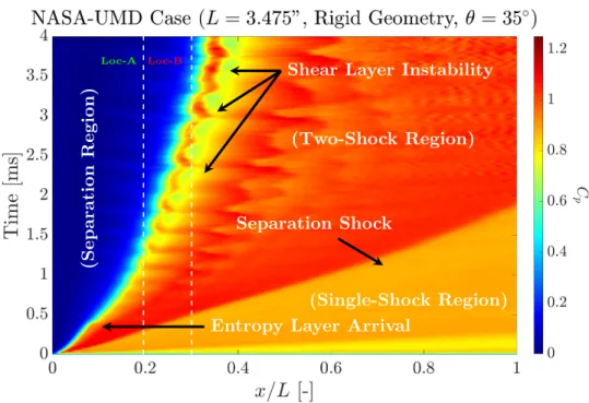
3.7 Rigid-Geometry Surface Pressure XT-plot . . . 33

3.8 Real and Imaginary Parts of Morlet wavelet withkψ= 13, Ashmead (2010) [61] 35 3.9 Time Series Analysis for x/L= [0.2,0.3], Rigid-Geometry Simulation . . . . 35

3.10 Time Series Analysis forx/L= [0.4,0.5], Rigid-Geometry Simulation . . . . 36

3.11 Verification of Normal Vector Calculation . . . 37

3.12 Computing the Traction Vector and Wall Shear Stress . . . 38

3.13 Rigid-Geometry Skin Friction . . . 39

3.14 Computing the Surface Heat Fluxq′′ w . . . 40

3.15 Rigid-Geometry Heat Transfer . . . 41

3.16 Evaluating Reynolds’ Analogy: Rigid-Geometry . . . 42

4.1 Normalized mode shapes and curvature for the first three linear modes . . . 46

4.2 Methods for Computing the Nonlinear Vibration Frequency . . . 55

4.3 Fluid and Solid Grids for Verification Test Case . . . 57

4.4 Low Kinetic-Energy Test Case, vmax=−0.1m/s . . . 58

4.5 High Kinetic-Energy Test Case, vmax=−2.0m/s. . . 58

5.1 Structured Grids for NASA-UMD Case (h= 0.032”) . . . 61

(10)

5.3 FTSI Simulation, Deflection and Velocity (h= 0.064”) . . . 63

5.7 Modal Decomposition of Panel Response (Isometric-View) . . . 66

5.8 Modal Decomposition of Panel Response (Top-View) . . . 67

5.9 Comparing Fundamental Frequencies for Compliant Panels . . . 68

5.10 Observed Compliant Panel Frequencies vs Deflection Amplitude . . . 69

5.11 Elastic Strain Energy Breakdown . . . 71

5.12 Panel Surface Pressure Coefficient - FTSI Simulation . . . 72

5.13 FTSI Simulation XT-plots,h= 0.032” . . . 73

5.18 Evaluating Reynolds’ Analogy: h= 0.032” . . . 77

5.23 Reynolds’ Analogy - Pressure Gradient Dependence . . . 79

5.24 Surface Temperature for h= 0.032” . . . 80

6.1 Direct Comparison of Reduced-Order Models for h= 0.032” . . . 82

6.6 Comparison of Reduced-Order Aero Models at 20% and 80% chord . . . 87

6.7 Key Features of the Two-Shock Compression Ramp Flow . . . 89

6.8 Corner Pressure Coefficient - Rigid geometry . . . 90

6.9 Surface Pressure XT-plots w/ Separation Model . . . 95

6.10 Comparison of Reduced-Order Models w/ Separation Model . . . 96

6.11 Accuracy of Reduced-Order Aero Models w/ Separation Model . . . 98

6.12 SE/LPT FSI Panel Response,h= 0.032” . . . 99

6.13 SE/LPT FSI XT-plots,h= 0.032” (continued) . . . 99

B.1 Sign Conventions for Beam-Aligned Coordinate System . . . 107

B.2 State of Uniaxial Stress . . . 109

C.1 Maximum of a Discretely-Sampled Continuous Function . . . 111

E.1 FTSI Simulation, Deflection and Velocity (h= 0.032”) . . . 122

(11)

E.6 Modal Decomposition (h= 0.032”) . . . 124

F.1 Comparison of Reduced-Order Aero Models atx/L= 50% chord . . . 125

F.2 Comparison of Reduced-Order Aero Models atx/L= 75% chord . . . 126

(12)

List of Abbreviations

AFOSR Air Force Office of Scientific Research

NASA National Aeronautics and Space Administration

WENO-JS Weighted Essentially Non-Oscillatory Scheme - Jiang & Shu

XPACC The Center for Exascale Simulation of Plasma-Coupled Combustion SWBLI Shock Wave Boundary Layer Interaction

CNS Compressible Navier-Stokes LaRC Langley Research Center

ROM Reduced-Order Model

FTSI Fluid-Thermal-Structural Interaction CFD Computational Fluid Dynamics DNS Direct Numerical Simulation UMD University of Maryland

GALCIT Graduate Aeronautical Laboratories at the California Institute of Technology CWT Continuous Wavelet Transform

AEDC Arnold Engineering Development Center VKF Von K´arm´an Gas Dynamics Facility SE/LPT Shock Expansion/Local Piston Theory LSI Local Surface Inclination

FFT Fast (Discrete) Fourier Transform LES Large-Eddy Simulation

RANS Reynolds-Averaged Navier-Stokes TACC Texas Advanced Computing Center CFL Courant-Friedrichs-Lewy

(13)

List of Symbols

Greek Symbols

γ specific heat ratio =Cp/Cv

ρ fluid density µ dynamic viscosity

ξ computational coordinates = (ξ, η, ζ)T ν kinematic viscosity, Poisson’s ratio λ eigenvalue, second coefficient of viscosity δ velocity boundary layer height (99%) θ1 ramp angle

Θ panel temperature

τij viscous stress tensor =µ(∂ui/∂xj +∂uj/∂xi) +λ∂uk/∂xkδij

σij Cauchy stress tensor =−pδij+τij

η deflection of the neutral plane ǫ axial strain

ψ wavelet function, transverse strain δij Kronecker delta function

β oblique shock wave angle, Mach scaling parameter ¯

χL hypersonic viscous interaction parameter =M∞3(C/Rex)1/2

Roman Symbols

C Chapman-Rubesin constant = ρwµw

ρ∞µ∞

(14)

P r Prandtl number Ch Stanton number = q ′′ w ρCpU∞∆T S RHS source term

Q vector of conserved variables = (ρ, ρu, ρv, ρw, ρE)T

u fluid velocity vector = (u, v, w)T

k thermal conductivity, reduced frequency J Jacobian

rg radius of gyration =

p I/A Z position of the panel surface

ˆ

P first Piola-Kirchoff stress tensor M Mach number

K hypersonic similarity parameter =M∞θ

E total energy per unit volume, modulus of elasticity F flux vector, deformation gradient tensor

I area moment of inertia

A cross-sectional area of the panel h compliant panel thickness b compliant panel lateral span L compliant panel length/chord

p thermodynamic pressure

q∞ freestream dynamic pressure = γ₂p∞M∞2

qi heat flux vector

r nozzle radius

Cf skin-friction coefficient

˜

Re∞ unit Reynolds number =ρ∞u∞/µ∞

Rex Reynolds number based on distance from leading edge

(15)

Subscripts & Superscripts (_·)∗ _{dimensional quantity}

(_·)0 initial condition

(_·)w conditions at the wall

(_·)e conditions at the boundary layer edge

(_·)∞ freestream flow conditions

(16)

Chapter 1

Introduction

1.1 Background & Motivation

Aircraft that experience sustained flight through the atmosphere at hypersonic speeds are exposed to a uniquely challenging aerothermal environment [1, 2]. The extreme dynamic pressure and temperatures presented by hypersonic flows present significant engineering challenges to nearly every facet of vehicle design. For thermal management, the vehicle must be made of strong, heat resistant materials, which tend be inconel-based and therefore heavy. Air-breathing hypersonic vehicles also feature heavily-integrated propulsion systems which an increase the pressure loading on the skin panels of the vehicle, as well as being particularly sensitive to angle of attack perturbations. A representative example of an air-breathing hypersonic vehicle is seen below in Figure 1.1.

Figure 1.1: Artist Rendering of the X-43B Hypersonic Aircraft, NASA [3]

Aircraft structures of hypersonic vehicles must be strong, lightweight, and typically multifunctional [4]. The intersection of competing requirements can result in situations where the effects of fluid-structure interaction (FSI) are significant. Moreover, the surface temperature distribution, which results from the aerothermal loading, changes both the mechanical response and the aerodynamic properties of the vehicle in flight. As such, a unified approach which accounts for the fluid, structural, and thermal aspects of the problem is required. This fluid-thermal-structural interaction (FTSI) which can occur in hypersonic

(17)

vehicles can be critical for their successful and reliable operation. The shock-dominated flows typical of hypersonic flight can exhibit interference effects and/or shock impingement that increases surface heat transfer rates exponentially.

The need for extreme care in the design of hypersonic vehicles was brought into sharp relief on the afternoon of October 3rd 1967, during what would become the fastest flight of the X-15 hypersonic research program. As is recounted by Watts [5,6] and Armstrong [7], ahead of this flight the rebuilt and heavily-modified second airframe X-15A-2 was fitted with a heat-resistant ablative skin coating, external fuel tanks, and a ventral dummy ramjet engine in preparation for a performance-envelope-expansion flight. Attaining an impressive Mach number of 6.7 and maximum altitude of 102,000 feet, it was discovered only after landing just how close test pilot Pete Knight came to experiencing a catastrophic failure in one of aviation’s most iconic aircraft.

(a) X-15A-2 after a test flight at Rogers Dry Lake, Watts (1968) [5]

(b) X-15A-2 with modifications for flight No. 2-53-97 w/ external fuel tanks and dummy ramjet, Armstrong (1969) [7] Figure 1.2: North American X-15A-2 Hypersonic Research Aircraft

A combination of shock impingement and interaction effects from the ventral fin of the scramjet resulted in increases in the surface heat transfer by an estimated factor ofh/h0= 7,

and an increase in pylon leading-edge heat-transfer coefficient by a factor of h/h0= 9 [6].

The temperature rise due to aerodynamic heating (estimated to be _≈2,700◦ F) caused several of the explosive bolts securing the scramjet in place to fire prematurely, eventually leading to structural failure of the single remaining bolt and causing the dummy scramjet to fall onto the test range below. Clearly, being able to predict the location and magnitude of peak aerothermal heating are critical to successful design of hypersonic vehicles.

(18)

In addition, the unsteadiness in shock-wave boundary-layer interactions (SWBLIs) has been identified as a possible source of excitation of compliant skin panels if frequency-matching occurs between the SWBLI and the compliant panel [8]. A canonical configuration which is known to generate a recirculation region is the self-interacting flow of a hypersonic compression corner, the relevant features of which are shown below in Figure 1.3.

Figure 1.3: Schematic of a hypersonic compression ramp configuration, Carter (1972) [9] The boundary layer growing on the flat plate section, in close proximity to the high-entropy layer (HEL) originating from the leading edge, encounters the adverse pressure gradient caused by the compression corner and separates from the surface. This separation creates isentropic compression waves at the foot of the separation region which coalesce into an oblique shock wave at the flow turns through a separation angleθsep. When the separated

shear layer encounters the ramp surface it turns the remainder of the ramp angle, forming another set of compression waves and an oblique shock at the reattachment point. The separation shock and reattachment shock may intersect in a triple-point (TP) if they are in sufficiently close proximity or at disparate enough wave angles. The shear layer, while not attached to the surface, gains kinetic energy from the mean flow which is converted into an impact over-pressure at reattachment[9]. The reattachment region may also see “necking” of the shear layer in the vicinity of the surface, which is associated with substantial increases in root-mean-squre surface pressure fluctuations and local heat transfer rates. Moreover, if the shear layer is thin enough for the shear instability mode not to be damped out, then the oscillations themselves will produce alternating compression and expansion waves above the separation region which propagate back to the panel and influence the subsequent pressure distribution. Beyond the high-frequency oscillations of the shear later (and general

(19)

unsteadiness from turbulence in the 3D case), the corner separation region has been shown to exhibit low-frequency limit cycle oscillations under certain conditions, the frequency of which may be low enough to couple resonantly with the vibration of the compliant panel.

As noted by Leyva [10], the fundamental challenges to hypersonic flight are myriad, including real gas effects and chemistry, transition to turbulence, second mode boundary layer instabilities, ablation, and fluid structure interaction. The ability to numerically simulate FTSI phenomena has been identified as a key growth area for informing structural design in terms of peak aerodynamic heating, maximum transient structural loads, and avoiding the risk of fatigue caused by excessive skin panel vibration or flutter. The present analysis aims to provide full-order, time-accurate FTSI simulation data for the dual purpose of understanding the physical mechanisms in this flow and provide data for validation to reduced-order models. The numerical simulations completed at the University of Illinois at Urbana–Champaign (UIUC) are performed in coordination with experimental efforts by a research team at the University of Maryland (UMD) to investigate a flat plate-ramp combination atM∞= 6.04 and unit Reynolds number Re∞= 23.6×106.

1.2 Literature Review

The breadth of literature on available on hypersonic research is positively vast, but we highlight some of the key research that is relevant to the compression ramp FTSI problem. To begin with, McNamara and Friedmann [11] provide an excellent survey of hypersonic aeroelastic and aerothermoelastic research directions in which future research efforts might travel. In particular, they conclude that the aim of sustained, reliable hypersonic flight will require the design of minimum-weight structures that can withstand an extreme aerothermal environment without the benefit of experimental data to validate the design. This places renewed emphasis on computational methods—both high-fidelity aerothermoelastic codes and reduced-order models—for robust and cost-efficient hypersonic vehicle design. Carter [9, 12] was one of the first to compute the viscous flow of a laminar boundary layer over a compression ramp at several Mach numbers, using the Brailovskaya finite-difference method while highlighting the potential sources of error caused by inappropriate boundary conditions. Mallinson [13] investigated the high-enthalpy, hypersonic flow over sharp leading edge compression corners at Mach numbers up to M∞= 9. Semi-empirical correlations for

upstream influence length, plateau pressure and reattachment pressure are provided and compared favorably to experimental data. Similar data was produced by Marini [14], with the focus on understanding the dependence of the SWBLI on the temperature ratio of the wall. Marini was found to provide the same semi-empirical correlations as Mallinson, in addition to some others. Three-dimensional DNS of the hypersonic compression ramp

(20)

flow, the structure of the hypersonic turbulent boundary layer was studied extensively by Smits [15], who used spectral 3D DNS data to study the turbulence structure angle and characteristic streamwise length scales of a turbulent boundary layer interacting with a rigid compression ramp. Stemmer [16] completed three-dimensional DNS of a rigid compression ramp in Mach 5 flow with real gas effects, and investigated the stability characteristics of both the separated shear layer and approaching boundary layer by computing Fourier modes of the resulting solution. Willems [17] used an experimental approach to study shock-induced FSI on a flexible wall in supersonic turbulent flow, in which the dynamic response of a compliant panel grazed by a turbulent supersonic flow was found to consist of both steady and dynamic components. The ideal of true two-dimensionality in the flow was not achieved due to finite-span effects and the high-frequency, small-amplitude oscillations showed a direct dependency to excitation by the flow.

Regarding aeroelastic research, Riley [18] highlighted the need for aerothermoelastic experimental data to be used for validation purposes, while providing an excellent overview of the typical challenges faced when attempting to aeroelastic data from speed, high-temperature wind tunnels. Experimental data are provided for a flexible test specimen tested in AEDC/VKF Tunnel C. Neely et al. [19] performed an experimental investigation of fluid-structure interaction of a cantilevered low-carbon steel plate in hypersonic flow at Mach 5.8. Measurements from both pressure transducers and pressure-sensitive paint (PSP) were compared directly with aerodynamic models such as piston theory (PT), quasi-steady piston theory, and the tangent wedge (TW) model. Analysis showed that there was negligible difference between PT and quasi-steady PT for the cases tested, and that the the TW model tended to over-predict the surface pressure. Pham et al. [20] were able to investigate the fluid-structure interaction between a compression ramp and flexible surface, but with this surface being a rubber sheet and positioned on the flat-plate section ahead of the ramp. A reduction of 50%-60% was observed in the energy content of shock oscillations with the embedded rubber layer versus an all-steel plate, suggesting properly tailored FTSI could be used as a viable tool for passive load mitigation. Casper [21] recently investigated the fluid-structure interactions of a compliant panel embedded in a 7◦ _{half-angle cone at}

the Sandia Hypersonic Tunnel at Mach 5 and 8 and the Purdue Boeing/AFOSR Mach 6 Quiet Tunnel. In this work, excitation of the compliant panel caused by turbulent spot generation was found to be over 200 times that of the excitation associated with the laminar boundary layer when the spot generation frequency coupled resonantly structural frequency of the panel. Gray et al. [22] developed high-order finite-element structural model with piston-theory aerodynamics to determine the nonlinear flutter characteristics of a two-dimensional simply-supported compliant panel grazed by a hypersonic flow.

(21)

of three-dimensional panel flutter in subsonic and supersonic flows. A three-dimensional viscous aeroelastic solver [23] was developed capable of computing three-dimensional mode shapes and associated surface pressure distributions of a compliant panel undergoing a limit cycle oscillation (LCO). The LCO amplitude and frequency were computed for both subsonic and supersonic Mach numbers for multiple panel aspect ratios, thicknesses, and freestream dynamic pressures. Among other results, it was determined that, for supersonic flows, the presence of the boundary layer was found to delay the onset of flutter to higher dynamic pressures, while simultaneously reducing the frequency of oscillation.

Figure 1.4: Surface pressure coefficient during LCO M∞= 1.2, Re= 1×105, Gordnier

and Visbal (2003) [24]

In Gordnier and Visbal 2003 [24], this work was extended to Re = 2_×105. It was demonstrated that the cavity pressure can have a pronounced effect one the on the flutter dynamics; a fact which becomes important when comparing simulation results to experiment. It was also shown that the delaying effect of the viscous boundary layer on flutter onset was more pronounced in the case of laminar boundary layers. Visbal [25] studied the interaction between an incident oblique shock and a flexible two-dimensional panel for inviscid flow, finding that the LCO amplitude and frequency both increase with shock strength at fixed dynamic pressure. The critical dynamic pressure for the emergence of an LCO was found to be considerably lower the standard panel flutter in certain cases, suggesting that an aeroelastic instability distinct from regular panel flutter is at play in this interaction.

(22)

McNamara et al. [26] generated reduced-order models to simulate the aerothermoelastic response of a simply-supported compliant panel located on the surface of a two-dimensional wedge in which SE/LPT is used to compute the unsteady surface pressure and Proper Orthogonal Decomposition (POD) based model reduction of CFD predictions to determine the surface heat flux. In a related paper, McNamara and Crowell [27] systematically evaluate several aerodynamic models for hypersonic flow including piston theory, Van Dyke’s second order theory, Newtonian impact theory, and unsteady shock-expansion theory in predicting flutter boundaries in comparison to an time-accurate Navier-Stokes solution. The Navier-Stokes solutions presented in this method assume that the general motion of the structure is described by a finite modal series, where the mode shape areassumedto be equal to the small-amplitude free vibration modes of the structure. The aeroelastic equations of motion are then obtained from Lagrange’s equations. More recently, Brouwer [28] compared the performance of CFD-enriched piston theory (EPT) against Euler and RANS simulations for shocks impinging on a compliant surface in 2D and 3D flows. The EPT results compared favorably to unsteady CFD for prescribed surface oscillations at orders of magnitude less computational cost. The effects of leading-edge bluntness and the presence of a high-entropy layer (HEL) on the flow-separation characteristics are significant as reported by Townsend [29], among others. A failure to properly scale the relative height of the entropy layer—generated at the leading edge—with the developing boundary layer on the flat plate is shown to significantly influence the size of the recirculation region and shear layer width.

1.3 Thesis Structure

In Chapter 2, we discuss the numerical methods and software tools utilized for the FTSI analysis, including the methods for solving the compressible Navier-Stokes (CNS) equations in generalized coordinates on moving grids, the WENO scheme used for advection in the fluid domain, the structural and thermal finite-element solvers, and reduced-order aerodynamic models. In Chapter 3, we test the CNS solver against a validation case, and investigate in detail the characteristics of the rigid-geometry hypersonic compression flow for the NASA-UMD case. Chapter4outlines methodologies for analytically-predicting the linear and nonlinear vibration frequencies of the compliant panel, as well was verifying the structural solver. Chapter5reviews in detail the results of FTSI simulations for various panel thicknesses, and in Chapter6the FTSI simulation results are quantitatively compared to reduced-order aerodynamic models. Chapter 7 summarizes the major findings of the present numerical analysis, as well as providing a road map for future work.

(23)

Chapter 2

Numerical Methods

2.1 Software Tools

McNamara and Friedmann [11] broadly classify the techniques of solving coupled fluid structure interaction problems as either monolithic (strongly coupled) or partitioned (weakly coupled). Monolithic solvers are identified by the formulation of a single system of equations for the fluid, structural, and thermal domains which are all solved simultaneously. A partitioned solver, conversely, solves the fluid, structural, and thermal domains independently (and possibly using different time steps), then passes information. By these definitions, the FTSI solver used for the current analysis is of the partitioned variety. PlasComCM is a multiphysics FORTRAN 90 code written primarily to solve the CNS equations, but with the capability to solve both structural and thermal problems as well. In the current work, three separate instances of PlasComCM are used to compute the solution in the fluid, solid, and thermal domains. The lion’s share of the computational work in the FTSI solver is performed in compiled code. This provides superior performance of large computational requirements of multi-physics solutions and optimization for the stated task. Because both the thermal and structural time integration methods are implicit, the fluid solution is estimated at the required intermediate times t = t+ ∆tst and t = t+ ∆tth

using a second-order Runge-Kutta scheme to advance the structural and thermal solutions respectively with 2nd-order accuracy.

The wrapper function written in Python is used to advance the fluid, structural, and thermal solutions in time while sharing boundary condition information between them. The Python coupler script—combined with FORTRAN 90 code to interface with the PlasComCM structural and thermal solvers—is entirely responsible for passing information between parallel solutions and enforcing the proper time-stepping between domains. Time steps for the fluid, structural, and thermal domains are integer multiples of each other, which implies that the timestep is constant for the duration of the simulation. This aspect is critical to the computational efficiency of the aerothermoelastic solver due to the disparate time scales present in FTSI calculations. The high-frequency content in the fluid solution requires a very small timestep for accurate calculation, which is contrasted with the low-frequency, long-period nature of the thermal solution. For representative geometry and material properties, the structural time step requirements are typically somewhere between these

(24)

extremes. The code is designed to be modular, such that the user can plug their solver of choice into the wrapper script independently of the other two domain solvers (for instance, to replace a CNS solution with a reduced-order aerodynamic model).

2.2 Fluid Domain Solver

2.2.1 Non-Dimensionalization

PlasComCM solves the compressible Navier-Stokes equations in non-dimensional form. Dimensional quantities are indicated by an asterisk (∗_{), while those quantities which are}

dimensionless are asterisk free. The reference variables used for non-dimensionalization are the freestream density ρ∗

∞, speed of sound c∗∞, dynamic viscosity µ∗∞ and Lref, a

characteristic length scale of the problem. The non-dimensional variables are then defined as follows: t= c ∗ ∞t∗ Lref xi = x∗ i Lref ρ= ρ ∗ ρ∗ ∞ (2.1) ui = u∗ i c∗ ∞ p= p ∗ ρ∗ ∞c∗∞2 µ= µ ∗ µ∗ ∞ (2.2) T = C ∗ p,∞T∗ c∗ ∞2 = T ∗ (γ∞−1)T∞∗ = γ∞p (γ∞−1)ρ . (2.3)

One benefit of this choice of non-dimensionalization is that the form of equation for the flow Mach number is unchanged. A noted consequence of this non-dimensionalization is the form given for the code Reynolds number, which is based on c∞:

Re= ρ ∗ ∞c∗∞Lref µ∗ ∞ , (2.4)

Similarly, the Prandtl number is defined as:

P r= C ∗ pµ∗∞ k∗ ∞ , (2.5) whereC∗

p is the specific heat at constant pressure andk∗∞is the fluid thermal conductivity

at the freestream condition. Thermally perfect, calorically perfect, and lookup-table gas models are available in PlasComCM. Due to the relatively mild stagnation enthalpy of the cases considered, the calorically-perfect model was used for the present calculations.

(25)

2.2.2 Conservation Equations

PlasComCM solves the compressible Navier-Stokes equations in curvilinear coordinates. The vector of conserved variables is composed of the densityρ, the momentum fluxρui, and

the total energy fluxρE. Using index form with the summation convention, the governing equations for mass, momentum, and energy become

∂ρ ∂t + ∂(ρuj) ∂xj =Sρ (2.6) ∂ρui ∂t + ∂ ∂xj (ρuiuj+pδij−τij) =Sρui (2.7) ∂ρE ∂t + ∂ ∂xj

[(ρE+p)uj+qj−uiτij] =SρE (2.8)

where p is the thermodynamic pressure, τij is the viscous stress tensor, qj represents the

heat flux vector, and Sρ, Sρui, and SρE are the source terms for mass, momentum, and energy, respectively. The equation of state is:

p= (γ₋1) ρE₋1 2ρ(u 2₊_v2₊_w2₎ . (2.9)

The PlasComCM fluid solver solves the CNS equations in generalized coordinates. Given a structured grid, it is possible to express the conservation equations for the fluid domain in a general curvilinear system ξi provided that the mapping Ξ fromxi toξi exists and is

well-defined. The Cartesian coordinates (x, t) can be mapped to another coordinate system (ξ, τ) via the time dependent mappings:

x=X(ξ, τ) with inverse ξ = Ξ(x, t) (2.10) where X−1 _{= Ξ and only non-singular maps are considered. For simplicity, we take} _t₌_τ_.

The Jacobian of the transformation is defined asJ = det(∂Ξi/∂xj) and is strictly positive.

Written explicitly, the Jacobian and grid metrics are:

J−1 =xξ(yηzζ−yζzη) +xη(yζzξ−yξzζ) +xζ(yξzη−yηzξ) (2.11) J−1    ξx ξy ξz ηx ηy ηz ζx ζy ζz   =    yηzζ−yζzη zηzζ−zζxη xηyζ−xζyη yζzξ−yξzζ zζxξ−zξxζ xζyξ−xξyζ yξzη−yηzξ zξxη−zηxξ xξyη−xηyξ    . (2.12)

(26)

Under these conditions and with simple application of the chain rule, it can be shown [30] that Eq.2.10 transforms to

∂ ∂τ Q J +∂Fˆ I i ∂ξi − ∂Fˆ_iV ∂ξi = S J (2.13)

after using the identities

∂ ∂ξj 1 J ∂ξj ∂xi = 0 fori= 1, . . . , N ∂ ∂τ 1 J + ∂ ∂ξj 1 J ∂ξj ∂t = 0, (2.14)

whereN is the number of dimensions. If we define a weighted metric ˆξi =J−1(∂ξ/∂xi) and

contravariant velocity ˆU =ujξˆj+ ˆξt, with similar expressions for the remaining components,

then the inviscid fluxes ˆF_iI in two dimensions are:

ˆ F₁I =       ρUˆ ρuUˆ +pξˆx ρvUˆ+pξˆy (ρE+p) ˆU₋ξˆtp       and Fˆ₂I =       ρVˆ ρuVˆ +pˆηx ρvVˆ +pηˆy (ρE+p) ˆV ₋ηˆtp       (2.15) and, ˆ F₁I =         ρUˆ ρuUˆ +pξˆx ρvUˆ +pξˆy ρwUˆ +pξˆz (p+ρE) ˆU₋ξˆtp         , Fˆ₂I =         ρVˆ ρuVˆ +pˆηx ρvVˆ +pˆηy ρwVˆ +pˆηz (p+ρE) ˆV ₋ηˆtp         and ˆF₃I =         ρWˆ ρuWˆ +pζˆx ρvWˆ +pζˆy ρwWˆ +pζˆz (p+ρE) ˆW ₋ζˆtp         (2.16) for the 3D case. The constitutive relation for the viscous stress tensor τij is given by:

τij = µ Re ∂ui ∂xj +∂uj ∂xi + λ Re ∂uk ∂xk δij (2.17)

where µand λ are the first and second coefficients of viscosity, respectively. The dynamic viscosity µand thermal conductivity kare allowed to vary with the thermodynamic state of the fluid. Given the large range of temperatures involved in the present calculations,

(27)

Sutherland’s law is employed to solve for the the fluid dynamic viscosity: µ(T) =µref T Tref 3/2 _T ref +S T+S , (2.18)

where µref = 1.715×10−5 kg/m-s, Tref = 273.11 K and S = 110.56 K. The viscous

terms may be either taken directly as ∂2/∂x2 or as two repeated derivatives ∂/∂x(∂/∂x). While mathematically equivalent, they differ numerically in terms of computational expense and physical dissipation apparent in the solution. Following Anderson, Tanehill, and Pletcher [31], the strong form of the viscous terms in two dimensions are given by:

∂ ∂t _ρu₁ J =_{· · ·} ∂ ∂ξ ˆ ξiτi1 + ∂ ∂η ˆ ηiτi1 ∂ ∂t _ρu₂ J =_{· · ·} ∂ ∂ξ ˆ ξiτi2 + ∂ ∂η ˆ ηiτi2 ∂ ∂t ρE J =_{· · ·} ∂ ∂ξ ˆ ξi[ujτij−qi] + ∂ ∂η ˆ ηi[ujτij−qi] , (2.19)

which is considerably faster than other available forms, but provides negligible dissipation at the highest wavenumbers. For the rigid-geometry case, the fluid solver is run at constant CFL, while the FTSI solver must be run at constant timestep.

2.2.3 Characteristic Boundary Conditions

For points on the boundary, we may use the characteristic wave relations to obtain the flux at that point. From Kim [32], the governing equations in the characteristic space are:

∂R

∂t +L=Sc, (2.20)

where R is the vector of characteristic terms and L is the vector of wave amplitudes. Equation 2.20is derived by the following two equations:

δR=P−1δQ, L=λ∂R ∂ξ =P −1 _ξ x∂ ˆ F₁I ∂ξ +ξy ∂Fˆ₂I ∂ξ +ξz ∂Fˆ₃I ∂ξ ! ;. (2.21) The source term S_c in Eq. 2.20can be related the source terms by:

Sc=JP−1 Sˆ_v− " ˆ F₁I ∂ ∂ξ ξx J + ˆF₂I ∂ ∂ξ(ξy) + ˆF I 3 ∂ ∂ξ ξz J +∂Fˆ ∂η + ∂Gˆ ∂ζ #! . (2.22)

(28)

Also note that ξx ∂E ∂ξ +ξy ∂F ∂ξ +ξz ∂G ∂ξ =J ∂Eˆ ∂ξ − E ∂ ∂ξ ξx J +F ∂ ∂ξ(ξy) +G ∂ ∂ξ ξz J ! . (2.23) The vector of characteristic differential variables and the corresponding wave speeds are

δR= δρ₋δp c2, δw, δ˜˜ v, δp ρc +δu,˜ ˜ p ρc−δu˜ T and (2.24) λ=hu, u, u, u+cqξ2 x+ξy2+ξz2, u−c q ξ2 x+ξy2+ξz2 iT , (2.25)

where the contravariant velocity in the direction normal to the boundary and its differential are given by:

u=ξxu+ξyv+ξzw (2.26)

δu˜= ˜ξxδu+ ˜ξyδv+ ˜ξzδw , (2.27)

and the velocity differentials in the parallel direction are given by

δv˜=₋ξ˜xδv+ ˜ξyδu (2.28)

δw˜=₋ξ˜xδw−ξ˜zδu . (2.29)

The “tilde” notation in this section indicates that a variable is normalized by the magnitude of the metric vector, such as:

h ˜ ξx,ξ˜y,ξ˜z i = q[ξx, ξy, ξz] ξ2 x+ξy2+ξz2 . (2.30)

The boundary derivative equation express in terms of the primitive variables is: ∂ρ ∂t +L1+ ρ 2c(L4+L5) =Sc1+ ρ 2c(Sc4+Sc5) (2.31) ∂u˜ ∂t + 1 2(L4−L5) = 1 2(Sc4−Sc5) (2.32) ∂˜v ∂t +L2=Sc2 (2.33) ∂w˜ ∂t +L3 =Sc3 (2.34)

(29)

∂p ∂t + ρc 2 (L4+L5) = ρc 2 (Sc4+Sc5), (2.35) where different types of boundary conditions (wall, perfectly-nonreflecting, etc.) can be specified by the appropriate choice of the incoming wave amplitudes L_i. Details regarding the exact procedure for setting these convection amplitudes are found in [32].

2.2.4 5th

-Order Finite-Difference WENO Scheme

In computing the fluid solution, the inviscid fluxes are computed using the 5th-order, finite-difference Weighted Non-Oscillatory (WENO) scheme of Jiang and Shu [33], with modifications for implementation on curvilinear grids. This special treatment for the inviscid fluxes was found to be necessary to ensure the stability of the fluid solver due to the presence of very strong shock waves in the hypersonic compression ramp solution. For simplicity consider using the WENO-JS scheme to solve the compressible Euler equations in one-dimensional flow, with the vector of conserved variablesQ and flux vectorF(Q) are given by: Q=    ρ ρu ρE    and F(Q) =    ρu p+ρu2 u(p+ρE)    . (2.36)

With zero source terms, the conservation equations can be written in vector form as ∂Q

∂t +

∂F(Q)

∂x = 0. (2.37)

The flux Jacobian is defined asA(Q) =∂F/∂Q and is equal to

A= ∂F ∂Q =      0 1 0 (γ₋3)u₂2 (3₋γ)u γ₋1 γ₋2 2 u 2₋ c2 γ₋1 u (3₋2γ)u 2 2 + c2 γ₋1 γu      , (2.38)

where c = pγp/ρ is the local sound speed. The characteristic decomposition of the flux Jacobian for the 1D Euler equations isA=RΛL, where Matsasuka [34] gives

(30)

Λ=    u₋c 0 0 0 u 0 0 0 u+c   , (2.39) R=      1 1 1 u₋c u u+c c2 γ₋1 + u2 2 −uc u2 2 c2 γ₋1+ u2 2 +uc      , and (2.40) L=         1 2 γ₋1 2c2 u 2₊u c −1₂ γ₋1 c2 u 2₊1 c γ₋1 2c2 1₋ γ−1 2c2 u 2 γ−1 c2 u 2 −γ_c−₂1 1 2 γ₋1 2c2 u 2 − u_c −1₂ γ₋1 c2 u 2 −1_c γ₋1 2c2         . (2.41)

Here Λ is the diagonal matrix of eigenvalues, and R and L are the matrices of right-and left-eigenvectors, respectively. Eigenvectors for the full 2D right-and 3D Euler equations for single-fluid and multi-component problems on curvilinear grids have been previously documented [35], and are reproduced in AppendixA.1. Simplifying further, consider solving the system of equations on a uniform gridxi =i∆x, and letQidenote the solution atx=xi.

The WENO-JS scheme for this system can then be written in flux-difference form: ∂Q ∂t i =₋ 1 ∆x ˆ F_i₊1 2 − ˆ F_i−1 2 . (2.42) In each case, ˆF_i₊1

2 is the numerical flux at the half-node grid point locations, which is

a WENO-reconstruction of the physical flux. The basic procedure for the numerical flux reconstruction is as follows:

1) Compute the physical flux at each grid pointxi:

Fi=F(Qi) (2.43)

2) At eachx_i₊1

2, compute and decompose the average Jacobian matrixAi+ 1 2: A_i₊1 2 = ∂F ∂Q i+1₂ =R_i₊1 2Λi+12Li+12, (2.44)

(31)

(column) eigenvectors, and L_i₊1

2 =R

−1

i+1₂ is the matrix of left (row) eigenvectors.

3) Project the solution and physical flux into the right eigenvector space: ˜ Qj =L_i₊1 2Qj and ˜ Fj =L_i₊1 2Fj (2.45)

for allj in the numerical stencil associated with associated withx=x_i₊1 2.

4) Perform a Lax-Friedrichs flux vector splitting for each component of the characteristic variables. Specifically, assume that the sth component of ˜Qj and ˜Fj are ˜Qj,s and ˜Fj,s

respectively, then compute ˜ F_j,s± = 1 2( ˜Fj,s±αsQ˜j,s), (2.46) where αs= max k |λs(Qk)| (2.47)

is the maximal wave speed of thesthcomponent of the characteristic variables over grid points 1_≤k_≤Nx for global flux splitting (ori−2≤k≤i+ 3 for local flux splitting)

and λs is the sth eigenvalue in the diagonal matrixΛ.

5) Perform a WENO reconstruction on each of the computed flux components ˜F_j,s± to obtain the corresponding component of the numerical flux. If we let ΦWENO5 denote

the fifth-order WENO reconstruction operator, then the flux is computed as follows: ˜

F+

i+1₂,s = ΦWENO5( ˜F

+

i−2,s,F˜i−+1,s,F˜i,s+,F˜i++1,s,F˜i++2,s), (2.48)

˜ F−

i+1 2,s

= ΦWENO5( ˜F_i−₊₃_,s,F˜_i−₊₂_,s,F˜_i−₊₁_,s,F˜_i,s−,F˜_i−−₁_,s). (2.49)

Then set ˜ F_i₊1 2,s = ˜F + i+1₂,s+ ˜F − i+1₂,s, (2.50) where ˜F_i₊1 2,s is the s th _{component of ˜}_F i+1₂.

6) Finally, project the numerical flux back to the conserved variables ˆ F_i₊1 2 =Ri+12 ˜ F_i₊1 2. (2.51)

The heart of the WENO scheme is the WENO reconstruction operator, denoted by ΦWENO5.

(32)

smoothness parameterβk. Consider a uniform grid withN + 1 grid points,

a=x0 < x1< . . . < xN+1 =b. (2.52)

We would like to compute the numerical flux ˆf_i₊1

2 of the “half-node” x=xi+ 1

2 by WENO

reconstruction on the stencil S = _{Ii−2, Ii−1, . . . , Ii+2}. For a 5th-order scheme, there

are three sub-stencils for node x_i₊1

2: S

0 ₌ _{_I

i−2, Ii−1, Ii}, S1 = {Ii−1, Ii.Ii+1} and S2 =

{Ii, Ii+1, Ii+2}. In each sub-stencilS_ik₊1 2

, the 3rd-order accurate numerical flux ˆf_ik₊1 2 is: ˆ f_i0₊1 2 = 1 3fi−2− 7 6fi−1+ 11 6 fi, (2.53) ˆ f_i1₊1 2 =₋1 6fi−1+ 5 6fi+ 1 3fi+1, (2.54) ˆ f_i2₊1 2 = 1 3fi+ 5 6fi+1− 1 6fi+2. (2.55)

The numerical approximation ˆf_i₊1

2 is defined as a linear convex combination of the above

three approximations: ˆ f_i₊1 2 =w0 ˆ f_i0₊1 2 +w1fˆ_i1₊1 2 +w2fˆ_i2₊1 2 , (2.56)

where the nonlinear weights are defined as wk= ˜ wk ˜ w0+ ˜w1+ ˜w2 , (2.57) ˜ w0 = 0.1 (ǫ+β0)2 , w˜1 = 0.6 (ǫ+β1)2 , w˜2 = 0.3 (ǫ+β2)2 . (2.58)

We take ǫ= 10−6 _{and the smoothness indicator parameters,}_β

k, are chosen as in Shu [36]:

β0 = 13 12 fi−2−2fi−1+fi 2 + 1 4 fi−2−4fi−1+ 3fi 2 , (2.59) β1 = 13 12 fi−1−2fi+fi+1 2 + 1 4 fi−1−fi+1 2 , (2.60) β2 = 13 12 fi−2fi+1+fi+2 2 + 1 4 3fi−4fi+1fi+2 2 . (2.61)

From these we define the fifth-order WENO reconstruction operator ΦWENO5 as follows:

ΦWENO5(fi−2, fi−1, fi, fi+1, fi+2) =w0fˆ_i0₊1 2 +w1fˆ_i1₊1 2 +w2fˆ_i2₊1 2 . (2.62)

(33)

2.3 Solid Domain Solver

A modified version of an existing non-linear, finite-strain FEM solver [37] is used for the solid domain. Consider general deformable body initially in a reference configuration B0, with

all points on the body defined by X. At some later time t, the translation, rotation, and deformation of the body can be described by the time-dependent mappingφ(X, t), such that every particle in the current configuration,B, can be written asx=φ(X, t) =X+u(x, t), whereu(x, t) is the displacement. Applying conservation of linear momentum to the current configuration, B, gives:

∇ ·σ+ρb=ρu¨, (2.63)

where σ is the Cauchy stress tensor, b is a field of any body forces (e.g. gravity ₋gk), ρ is the solid density, ¨u =∂2u/∂t2 is the acceleration, and _∇ is the gradient in the current configuration. The deformation gradient is then defined as:

F(X, t) =_∇Xφ(X, t) = ∂x

∂X, (2.64)

where the Jacobian of the deformation gradient J = det(F) is equal to the volume change between reference and current configurations. If a virtual displacement δu is applied and Eq. 2.63 integrated over tho body in configuration B, the weak form of the principle of virtual work is:

δW = Z B (_{∇ ·}σ)_·δudv+ Z B ρb_·δudv₋ Z B ρu¨_·δudv = 0. (2.65) The divergence theoremR_v_{∇ ·}( )dv=R_δv( )_·nˆ can be used to write Eq.2.65 as,

δW = Z B σ:∇δudv+ Z B ρu¨_·δudv₋ Z ∂Bt T(n)_·δuda₋ Z B ρb_·δudv =0, (2.66) where T(n) =σ·nˆ is the traction vector applied to the the deformed boundary∂Bt with

outward pointing normal vector ˆn. The solver applies the principle of virtual work to the reference configuration B0, which necessarily requires a transformation. Pulling back

Eq. 2.66 to the reference configuration, the complete details of which can be found in Ostoich [37], result in the following expression for the variation of virtual workδW:

δW = Z B0 β2(Θ) ˆP :δF dV + Z B0 ρ0u¨·δudV − Z ∂B0 T₀(n)_·δudA₋ Z B0 b0·δudV =0, (2.67)

(34)

whereF is the deformation gradient tensor as defined by Eq. 2.64, the productβ2_{(Θ) ˆ}_P _is

the first Piola-Kirchoff stress tensor multiplied with the linear stretch ratio due to thermal expansion/contraction. In solving the nonlinear problem, if the current configuration of the body does not satisfy δW(u) = 0, then δW is linearized at u and multiplied by a correction ∆u to achieve δW(u+ ∆u) = 0. The corrected configuration u+ ∆u is then found iteratively through Newton iteration. Displacement, velocity, and acceleration are stored at 20 nodal locations per element using quadratic shape functions. Discretization of the linearized equation results in:

Mu¨+K∆u=Rext₋Rint, (2.68) whereRextandRintare the external and internal load vectors (respectively),K andM are the tangent stiffness and mass matrices, ¨uanduare the nodal acceleration and displacement vectors, and ∆u is the linear correction term. The dynamic equilibrium equation at time step n+ 1 is:

Rint_n₊₁₋Rext+Mu¨n+1=0. (2.69)

Temporal advancement of Eq.2.69is accomplished using a second-order, A-stable Newmark-β method [38] written as:

u_n₊₁ =u_n+ ∆tsu˙n+

∆t2_s

4 [(1−2β) ¨un+ 2βu¨n+1], (2.70) ˙

un+1 = ˙un+ ∆ts[(1−γ) ¨un+γu¨n+1], (2.71)

with specific valuesγ = 1/2 and β= 1/4 chosen to maximize accuracy. The finite-element structural model does not account for any structural damping or plastic deformation.

2.4 Thermal Solver

The thermal solution for the solid temperature Θ is found by numerically-solving the transient heat equation in the current configuration, B,

ρCpΘ +˙ ∇ ·q= 0, (2.72)

where Θ is the temperature of the panel,q is the heat flux vector, Cp is the thermal heat

(35)

Z B ρCpΘδΘdv˙ + Z B (_{∇ ·}q)δΘdv= 0 (2.73) =_⇒ Z B ρCpΘδΘdv˙ − Z B q_·δΘdv+ Z ∂B q_·nδΘda= 0, (2.74) whereδΘ is the arbitrary weight function and the divergence theorem has been applied to achieve the form of Eq. 2.74. Eq.2.74 can be brought back to the reference configuration B0 and discretized to give the governing equation for the thermal solution,

CthΘ˙ +KthΘ=Rth. (2.75)

whereΘis the temperature vector,C_th andK_th are the thermal capacitance and stiffness, respectively, andRth is the thermal load vector. The thermal solution is advanced in time

using the Crank-Nicholson scheme using the trapezoidal rule. A more detailed description of the spatial and temporal discretization of Eq.2.72 can be found in Ostoich [37].

2.5 Interface Treatment

The fluid, solid, and thermal domains are weakly coupled at the interaction boundary. Nodes are collocated on the fluid and solid sides of the interface, allowing for direct transfer of information without a spatial interpolation step. At each node, the full fluid stress tensor σ = ₋pI +τ and wall heat flux q′′ ₌ ₋_k_∇_T _·_n_ˆ _{are passed to the structural and}

thermal domains, respectively. The structural domain passes the positionxto the fluid and thermal domains, while additionally passing the surface velocity ˙xto the fluid domain. The thermal domain passes the temperature Ts back to the fluid and solid domains. A visual

representation of the interface data communication is provided below in Figure2.1.

Thermal Structural Fluid Ts Ts ds x s_, ∂_x s ∂_t t = σ f ·_n_ˆ q ′′ = −∇ Tf· ˆ n

(36)

2.6 Deformation of Fluid-Domain Grid

In computing an accurate fluid solution near the dynamically-moving interface boundary condition, it is necessary to deform the entire fluid grid in a computationally way. An arclength-preserving trans-finite interpolation (TFI) is used to deform the interior of the fluid grid in response to deformation at the boundary due to the structural solution. The precise details of of the TFI grid interpolation can be found in Spekreijse [39]. A qualitative representation of the deformation of a curvilinear grid due to motion at its boundary is given below in Figure2.2. Here the solid domain is colored blue while the interacting interface is green; the larger fluid domain is colored black.

Figure 2.2: Qualitative illustration of conforming fluid grid (black), solid domain grid (blue), and interacting boundary (green) using TFI

2.7 Reduced-Order Aerodynamic Models

Absent the numerically-complex and computationally-intense computation of a full-order numerical simulation of the CNS equations for hypersonic flow, a wide array of reduced-order models (ROMs) are available to approximate the unsteady pressure distribution. These include, but are not limited to, Newtonian impact theory, tangent wedge (TW) theory, Van Dyke’s second order theory, classical piston theory (CPT), and local piston theory (LPT). A brief discussion of each of the ROMs included in the present work is included in Sections2.7.1through2.7.4. The Matlab implementation of these models is included in for reference AppendixD. An equivalent code was written in Python to properly integrate into the coupled FTSI solver.

(37)

2.7.1 Newtonian Impact Theory

One of the oldest models for describing the pressure created by a moving fluid flow is attributed to Isaac Newton, dating back to the publishing of hisPrincipiain 1687. Although ultimately proven to be inaccurate for everyday low-speed flows, it remains a reasonable starting point for predicting surface pressure in hypersonic flows, with it’s accuracy increasing in the limit of high freestream Mach numbers and specific heat ratios approaching unity [2]. Applying conservation of linear momentum to a streamtube in the direction normal to the surface gives:

(ρ∞U∞·nˆ)(U∞−Us) = (ps−p∞) ˆn, (2.76)

where Us is the velocity vector adjacent to the wall, ˆn is the surface normal vector, and

ps is the surface pressure which we wish to compute. Impact theory assumes complete

annihilation of the normal component of the momentum at the wall, thus: ps=p∞+ρ∞(U∞·nˆ)2 =p∞ 1 +γM_∞2 sin2 tan−1 ∂Z ∂x . (2.77)

The slope of the surface (in this case∂Z(x, t)/∂x) is computed using Fornberg’s method [40] for computing derivatives on arbitrarily-spaced 1D grids. In locations along the surface whereU_∞·nˆ _≥0 (i.e. expansion regions), the pressure is set equal to the freestream value.

2.7.2 Tangent Wedge Theory

For a slender body at high Mach number, a more refined estimation of the surface pressure can be made using tangent wedge (TW) theory [2, 19, 41]. The TW method, similar to Newton’s impact model, is another local-surface inclination method which uses only the local slope of the surface to determine the pressure. Instead of assuming annihilation of the normal component of the freestream momentum, the TW method instead makes the assumption that the surface pressure is locally equal to the pressure of a two-dimensional wedge with the same slope; the surface pressure is then computed from an oblique shock solution. For relatively slender angles and high Mach numbers, the oblique shock pressure ratio can be approximated in explicit form:

ps p∞ = 1 +γ(γ+ 1) 4 K 2₊_γK2 s γ+ 1 4 2 + 1 K2 , (2.78)

(38)

where K=M∞θs is the hypersonic similarity parameter and θs is the local surface angle

relative to the freestream direction in radians. The local surface angle can be computed from the local slope as tan(θs) = ∂Z(x, t)/∂x, where again Fornberg’s method is used to

compute the derivatives.

2.7.3 Classical Piston Theory

The starting point for all forms of piston theory can be considered Hayes’ [42] hypersonic similitude principle for slender bodies, which is known variously as the “unsteady analogy,” or “hypersonic equivalence principle.” This principle stated directly is that, for a slender body moving at high Mach number, the disturbance generated by the shape of the body can be considered to act in a series of independent planes which are normal to the freestream flow direction. Lighthill [43] was one of the first to apply this principle to oscillating airfoils, resulting in what today is known as Classical Piston Theory. Meijer [44] has provided an excellent overview of the history or piston theory and advancements made on the basic concept. All piston theory models require calculation of an equivalent piston velocity,

Vp =U∞

∂Z(x, t) ∂x1

+∂Z(x, t)

∂t , (2.79)

where Z(x, t) is the unsteady panel response. The spatial index x1 indicates that the

panel slope is measured relative to the freestream (horizontal) direction. Upon inspection, equivalent 1D piston velocity is seen to be composed of the transient motion of the surface itself ˙Z(x, t), combined with an advective term which depends on the product of the freestream velocity U∞ and local surface inclination Z′(x, t). For an isentropic flow, the

pressure-velocity relationship is: p p∞ = 1 +γ−1 2 Vp a∞ 2γ γ−1 . (2.80)

Lighthill showed that the major compression/expansion effects can be replicated by a 3rd_{-order approximation to Eq.}_2.80:

ps p∞ = 1 +γ " Vp c∞ +γ+ 1 4 Vp c∞ 2 +γ+ 1 12 Vp c∞ 3 # = 1 +γ Mp+ γ+ 1 4 M 2 p + γ+ 1 12 M 3 p (2.81) =_⇒ ps p∞ = 1 +γ c1Mp+c2Mp2+c3Mp2 , (2.82)

(39)

whereMp∞=Vp/c∞ is the equivalent piston Mach number based on the freestream sound

speed. Improvements to this basic model—first by employing second-order supersonic potential theory and followed by a method of characteristics solution—were developed by Van Dyke [45] and Donov [46], respectively. It can be shown that the results of these analyses can also be written in terms of an expansion inMp. Thus, Eq.2.82can be used to

describe several different reduced-order aerodynamic models for hypersonic flow, depending on the particular set of coefficients chosen. Table2.1below shows the coefficients associated with the models of Lighthill, Van Dyke, and Donov.

Table 2.1: Piston Theory Coefficients (m=√M2₋₁₎

Term Lighthill Van Dyke Donov

c1 1 M/m M/m c2 γ+ 1 4 (γ+ 1)M4₋4m2 4m4 (γ+ 1)M4₋4m2 4m4 c3 γ+ 1 12 0 (γ+1)M8₊₍₂_γ2₋₇_γ−₅₎₊₁₀₍_γ₊₁₎_M4₋₁₂_M2₊₈ 12M m7

Reference conditions for classical piston theory are thefreestreamconditions. The description of CPT is included here mainly to provide context for the SE/LPT models. Preliminary calculations for CPT applied to the θ1 = 35◦ NASA-UMD case (where the turning angle

is well-beyond the small-angle assumptions used in deriving CPT) suggest relative error in predicated surface pressure values ranging from 80%-120%.

2.7.4 Shock-Expansion/Local Piston Theory

While CPT has proven itself an impressively-accurate tool for predicting the surface pressure around slender bodies at high Mach numbers, the requirement that unsteady surface pressure ps(x, t) be expressed as a perturbation of the freestream pressure is a restrictive limitation,

especially for large deflection angles and lower Mach numbers. A natural extension of CPT, then, is to precompute the local flow conditions (static pressure, speed of sound, etc.) at the desired position along the surface, then express the unsteady surface pressure as a perturbation to this local fluid state. That is to say,

ps ploc = 1 +γ " Vp aloc +γ+ 1 4 Vp aloc 2 +γ+ 1 12 Vp aloc 3 # = 1 +γ c1M˜p+c2M˜p2+c3M˜p2 , (2.83)

(40)

where ˜Mp = Vp/aloc is the equivalent piston Mach number based on the local speed of

sound. Local quantities can originate from any source, including shock-expansion theory, inviscid Euler solutions, or viscous simulations such as RANS or LES. For the purposes of the present work—where a compression-ramp defines the base flow properties—standard shock expansion-theory is used to determine the assumed local flow conditions immediately adjacent to the ramp surface. We will refer generally to local piston theory with reference conditions computed using shock-expansion theory as SE/LPT. If State-1 and State-2 are the pre- and post-shock flow states, then the oblique shock equations are [2,47]:

tanθ1 = M₁2_n₋1 tanβs1 + (γ+ cos 2βs)M12/2 (2.84) p21= p2 p1 = 2γM 2 1n−(γ−1) γ+ 1 (2.85) ρ21= ρ2 ρ1 = (γ+ 1)M 2 1n 2+(γ₋1)M2 1n (2.86) T21= T2 T1 = p21 ρ21 = 2γM2 1n−(γ−1) γ+ 1 2+(γ₋1)M2 1n (γ+ 1)M2 1n (2.87) M2n= s 2 + (γ₋1)M2 1n 2γM2 1n−(γ −1) (2.88) M2 = M2n sin(β_s−θ1) , (2.89)

where θ1 is the ramp angle, βs the wave angle, and M1n=M1sinβs. In computing the

LPT equivalent piston velocity, we require knowledge of both the panel slope and velocity in a ramp-aligned reference frame. Letting the slope of the panel in the rotated frame be indicated by x2, the ramp-aligned slope is related to the slope in the original frame by:

∂Z ∂x2 = tan tan−1 ∂Z ∂x1 −θ1 = ∂Z ∂x1 − tan(θ1) 1 + ∂Z ∂x1 tan(θ1) . (2.90)

Machine-precise solutions to Eq.2.84 are obtained using Newton-Raphson iteration, where the complex-step derivative (CSD) approach of Martins et al. [48] is used to evaluate the gradient of the residual function without explicit knowledge of the function.

(41)

Chapter 3

Rigid-Geometry Hypersonic Flow

Simulations

In the build-up to a full FTSI simulation of the UMD target application of a compliant panel embedded in a hypersonic compression ramp flow, two rigid-geometry simulations were first conducted. The first of these is to verify and validate the solver results for a hypersonic compression ramp flow at representative Mach number and Reynolds number. The second is a rigid-geometry simulation of the UMD case at the true flow conditions to form a baseline against which to compare the later FTSI simulations.

3.1 RWTH-Aachen Validation Case

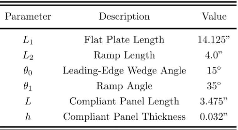
Several potential sources for hypersonic compression ramp experimental data are available in the literature [14,49,50,51,52]. One case which seemed especially promising was that of Reinartz et al. [53] studying the influence of SWBLIs in hypersonic intake flows. This paper provides experimental data collected by Bleilebens [49] in direct comparison with CFD calculations using a RANS solver. The selected test case has a 15◦ compression ramp at “Condition-I” with M∞ = 7.7 and Re∞L = 4.368×105. The flat plate length for the

RWTH-Aachen case isL= 0.105 meters, with ramp lengthLr = 0.163 meters. A summary

of the freestream flow conditions is given below in Table 3.1.

Table 3.1: RWTH-Aachen Freestream Conditions

M∞ [-] Re [-] ρ∞[kg/m3] p∞ [Pa] T∞ [K] c∞[m/s] u∞ [m/s]

7.7 4.368_×105 _0.02086 ₇₄₈ ₁₂₅ _224.1 _1725.34

An 897_×345 grid was created with grid spacing prescribed to enforce ∆y+ _< _{1.0 and}

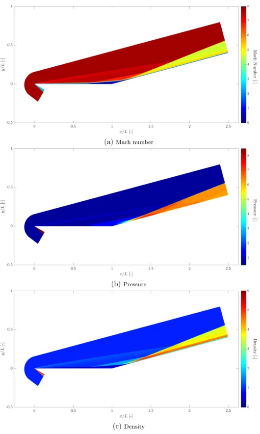
∆x+<20. From evaluation of several different configurations, it was determined to model the leading edge explicitly, as opposed to utilizing a discontinuous boundary condition along one side of a rectangular domain. The simulation was determined to reach steady state by a non-dimensional time of t =t∗_L/U

∞ = 0.173636. Plots of the Mach number, pressure,

(42)

(a)Mach number

(b)Pressure

(c) Density

(43)

Each of the qualitative flow features we expect to see from the hypersonic compression ramp problem are present in the RWTH-Aachen solution. We observe a detached leading edge shock extends out to a weak oblique shock as the distance from the leading edge increases. We observe a separation region, separated shear layer, “necking” of boundary layer after reattachment, and the formation of a triple-point where the separation shock and reattachment shock intersect. Turning to a more quantitative assessment, we produce line plots of the surface pressure coefficient Cp = (p−p∞)/q∞ as a function of distance

along the flat plate/ramp combination in Figure3.2.

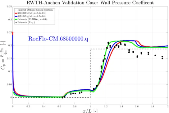
Figure 3.2: Comparison of Surface Pressure Coefficient

Four data sets are plotted in Figure3.2: PlasComCM solutions on 647_×300 and 897_×345 grids, simulation data from the FLOWer RANS solver, and experimental data from Reinartz et al. [53]. We note that PlasComCM appears to do a very good job at predicting the separation location, separation pressure, and reattachment pressure. It also does a good job in the recovery (aft) region where the pressure asymptotically approaches the inviscid oblique shock value. The major area of discrepancy between the experimental data and the FLOWer solver seems to be the width of the pressure ride region from the separation pressure to the plateau pressure. From an investigation of the flow field, this discrepancy is believed to be due to combined height of the shear layer/high-entropy layer being larger in the experimental data or the FLOWer prediction. Finally, we observe that both PlasComCM and FLOWer over-predict the pressure downstream of the plateau region. Reinartz [53]