Learning Edit Cost Estimation Models for Graph Edit Distance

HAL Id: hal-02285793

https://hal.archives-ouvertes.fr/hal-02285793

Submitted on 13 Sep 2019

HAL

is a multi-disciplinary open access

archive for the deposit and dissemination of

sci-entific research documents, whether they are

pub-lished or not. The documents may come from

teaching and research institutions in France or

abroad, or from public or private research centers.

L’archive ouverte pluridisciplinaire

HAL, est

destinée au dépôt et à la diffusion de documents

scientifiques de niveau recherche, publiés ou non,

émanant des établissements d’enseignement et de

recherche français ou étrangers, des laboratoires

publics ou privés.

Learning Edit Cost Estimation Models for Graph Edit

Distance

Xavier Cortés, Donatello Conte, Hubert Cardot

To cite this version:

Xavier Cortés, Donatello Conte, Hubert Cardot.

Learning Edit Cost Estimation

Mod-els for Graph Edit Distance.

Pattern Recognition Letters, Elsevier, 2019, 125, pp.256-263.

Learning Edit Cost Estimation Models for Graph Edit Distance

XavierCort´esa_{, DonatelloConte}a,∗_{, HubertCardot}a

a_{Universit´e de Tours, Laboratoire d’Informatique Fondamentale et Appliqu´ee de Tours (LIFAT - EA 6300), 64 Avenue Jean Portalis, 37000 Tours, France}

ABSTRACT

One of the most popular distance measures between a pair of graphs is the Graph Edit Distance. This approach consists of finding a set of edit operations that completely transforms a graph into another. Edit costs are introduced in order to penalize the distortion that each edit operation introduces. Then, one basic requirement when we design a Graph Edit Distance algorithm, is to define the appropriate edit cost functions. On the other hand, Machine Learning algorithms has been applied in many contexts showing impressive results, due, among other things, its ability to find correlations between input and output values. The aim of this paper is to bring the potentialities of Machine Learning to the Graph Edit Distance problem presenting a general framework in which this kind of algorithms are used to estimate the edit costs values for node substitutions.

1. Introduction

Machine Learning (ML) is now used in many research fields, given its potential and efficiency. Even when the final task is not classification, machine learning is still used in some part of the processing chain in order to effectively respond to certain problems that arise (e.g. fixing meta-parameters of a framework).

This is the case dealt with in this paper: we want to show how learning tools can help to solve some specific issues in the general

context of Structural Pattern Recognition, and more in particular for Graph Edit Distance Problem.

Graphs are defined by a set of nodes (local components) and edges (the structural relations between them), allowing to represent

the connections that exist between the component parts of an object. Due to this, graphs have become very important to model

objects that require this kind of representation. In fields like cheminformatics, bioinformatics, computer vision and many others,

graphs are commonly used to represent and classify objects (Conte et al., 2004;?;?;?). One of the key points in pattern recognition

∗_{Corresponding author}

is to define an adequate metric to estimate distances between two patterns. The Error-tolerant Graph Matching tries to address this

problem. In particular, the Graph Edit Distance (GED) problem (Bunke H., 1983;?) is an approach to solve the Error-tolerant

Graph Matching problem by means of a set of edit operations including insertions, deletions and node substitutions.

In the context of GED, one of the issues to solve is to fix edit cost functions to obtain a good dissimilarity measure between two

graphs.

The purpose of this paper is twofold:

• First, to propose a framework in which a machine learning tool is inserted in the processing chain for computing GED, in

order to obtain more accurate solutions than existing methods;

• Second, to analyze the impact, in terms of time processing and accuracy, of different machine learning algorithms on the solution of GED.

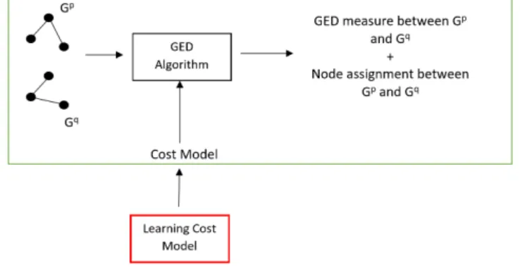
Fig. 1. The general scheme of learning costs for GED problem.

The classic schema for GED computation is depicted in the green box of Figure 1: given two graphs, a GED algorithm is applied

based on somefixed cost models between nodes; the GED algorithm provide the GED measure and the association between the

nodes of the two graphs, according to the given cost model. In this paper we want to discuss the introduction of a ML module that

providesbettercost models, avoiding to fix ita priori.

A first tentative in this direction was presented in (Cort´es et al., 2018) in which the use of a Deep Neural Network (DNN) for

parameters regression to compute assignment costs for GED has been shown. This paper is a continuation of that work with the

The introduction of the ML module in the context of GED is shown in Figure 1 (red box) and will be discussed in the next

sections.

2. State of the Art

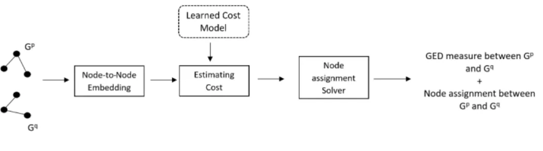
Fig. 2. Proposed framework to compute the GED with a learned model for edit cost estimation.

The output of the GED depends on the edit costs, that is, the distances cost for substituting a pair of nodes, and the penalties

costs for insertions and deletions. Typically, these costs are tied to cost functions defineda priori. Depending on how these costs

functions are defined the performance can be different either in terms of graph classification accuracy or in terms graph matching accuracy between the automatically estimated node-to-node correspondence and a ground truth correspondence. Recently, in order

to increase the performance of different Error-Tolerant Graph Matching approaches including the GED, some researchers have been working on automatically learning the parameters involved in these models instead of using the traditional trial-error method since

it can be very costly and not exhaustive. We can separate these approaches in three main groups depending on its goal. By one hand,

the first group (Raveaux R., 2017; Neuhaus and Bunke, 2005, 2007; Leordeanu et al., 2012) focuses on the graph classification ratio,

while the second group (Caetano et al., 2009; Cort´es and Serratosa, 2016; Serratosa F., 2011; Cort´es and Serratosa, 2015;?) targets

the node-to-node matching accuracy. Finally, there is a particular case in (Riesen K., 2016) that does not learn the parameters or

costs functions to improve the performance of the model but tries to predict if an edit operation is correct or not depending on the

values of the cost matrix. Moreover, another subdivision can be considered depending if the methods learn substitution costs or

insertions and deletions.

The aim of our paper is to propose a model to estimate the substitution costs, maximizing the graph matching accuracy, exactly

the nodes to apply after the weighted Euclidean distance. However, our work goes a step further, bringing the advantages of ML

algorithms. Because our framework is not tied to a specific cost function, it is able to generalize and find deeper correlations between

node attributes when estimating substitution costs. As we have mentioned in the introduction, this paper is the continuation of a

preliminary work presented in (Cort´es et al., 2018). We propose to analyze more in depth the consequences of introducing a ML

module for computing GED. In the experimental section we show how it can be combined with several ML algorithms, presenting

a very good performance for many of them.

3. Definitions and Methods

This section introduces some definitions and methods necessary to understand the paper. In Table 1 we summarize the main

notations.

Table 1. Main notations. G: Generic attributed graph.

Σv: Set of nodes inG.

vi: NodeithofG.

Σe: Set of edges inG.

ei j: Edge connecting nodeithto node jthofG.

γv: Function that maps nodes to their attributed values.

γe: Function that maps the structure of the nodes.

f: Function that maps nodes between two graphs.

c: Cost function of an edit operation.

cv: Local distance measure between a pair of nodes.

ce: Structural distance measure between a pair of nodes

Ψ: Vector containing the attributes of a node.

E: Function mapping the degree of a node.

x: Embedded representation of an edit operation.

y: Predicted value through an edit cost estimation model.

o: Ground-truth output value of an edit operation.

3.1. Attributed Graph

Formally, we define an attributed graph as a quadrupletG = (Σv,Σe, γv, γe), whereΣv ={vi|i =1, . . . ,n}is the set of nodes,

maps the structure of the nodes.

3.2. Graph Correspondence

We define a correspondence between two graphsGpandGqas a bijective function f :Σvp→Σ q

vthat assigns the nodes ofGpto

the nodes ofGq. Where f(v_ip)=vq_j, if a mapping betweenvp_i andvq_jexist.

3.3. Edit Costs for Graphs Edit Distance

The basic idea of the GED (Bunke H., 1983) between two graphsGpandGq, is to find the minimum cost to transformGpintoGq

by means of a set of edit operations, including insertions, deletions and node substitutions, commonly referred to aseditpath. And

editpath, can be directly related to a graph correspondence, by mapping the nodes involved in each edit operation. Cost functions

are introduced to quantitatively evaluate the level of distortion that each edit operation introduces.

cv_ip→vq_j=cv

v_ip→vq_j+ce

v_ip→vq_j (1)

The cost of a substitution edit operation (1) is typically given by the distance measure between the nodes attributescv

v_ip→vq_j= local distanceγvp v_ip, γqv

vq_jand by the cost of substituting the local structuresce

v_ip→vq_j=structural distanceγep v_ip, γqe vq_j.

These cost functions estimate the degree of dissimilarity between a pair of nodesv_ipandvq_jbelonging to graphsGpandGq. The

Eu-clidean distance is a common way to estimate thelocal distancebetween the nodes attributes, while in (Serratosa and Cort´es, 2015)

different metrics are presented to estimate the structural distance. In our framework, the idea is to automatically learn a model that estimates these costs, from a collection of training correspondences previously labeled, instead of having to define it manually.

When graphs have different cardinality, they can be extended with null nodes adding penalty costs (insertions and deletions) when an existing node of one graph is substituted by a null one of the other graph. In this paper we do not consider this option since

we focus on the problem of nodes substitution cost, comparing our results with other works that face exactly the same problem, as

in (Caetano et al., 2009; Cort´es and Serratosa, 2016). However, our framework can be extended to consider null nodes by adding

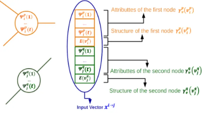
Fig. 3. An illustration showing the embedding process of two nodes (orange and green) into an input vector.

4. Proposed Framework

In this section we present a new framework to compute the GED between a pair of graphs with a model to estimate edit cost,

previously learned.

The framework schema is shown in Figure 2; given two graphs (Gp,Gq), each pair of nodes (v_ip,vq_j) is embedded in a real-valued vector (Subsection 4.1), then the vector is passed to a ML model (who is learned following the approach described in

Subsection 4.2), finally, an assignment solver is used to obtain the optimal (or sub-optimal) node-to-node correspondence between

nodes and the total graph matching cost value (Subsection 4.3).

4.1. Node-to-Node Embedding

The first step of our model consists of transforming the local and structural information of two nodes into a set of inputs for the

ML model that estimates the edit cost of substituting both nodes. In this section we show how to embed this information.

LetGp_andGq_{two attributed graphs,γ}p v =

n

vp_i →Ψ_ip|i=1, . . . ,noa function that assignstattribute values from an arbitrary do-main to each node ofGp_{, whereΨ}p

i ∈R

t_{is defined in a metric space oft∈}

Rdimensions andγep=

n

vp_i →E(v_ip)|i=1, . . . ,nowhere

E(·) refers to the number of edges incident on a certain node. And similar forγvqandγ p einGq. Vectorxi→j= h γp v(v p i), γ p e(v p i), γ q v(v q j), γ q e(vq_j)i∈

R(t+1)×2is the embedded representation of the assignmentvip→v q

jwhere the vectorx

i→j_{corresponds to the set of inputs of the ML}

algorithm that estimates the cost of substituting nodev_ipofGp_{by nodev}q jofG

Fig. 4. (a) Correspondence between a pair of graphs. Colored circles: Nodes. Black lines: Edges. Green arrows: Graph correspondence. (b) Set of all possible node substitutions and expected costs given the correspondence in (a).

4.2. Training the Model

We follow a supervised learning approach to treat the problem of training the edit cost estimation model. The training set has

Kobservations composed by a triplet consisting of pair of graphs and the correspondence that relates its nodes{Gpk,Gqk,fk}. The ground-truth correspondences fk must be provided by an oracle, generally a human expert, according to the nature of the graphs

(images, fingerprints, letters,etc.).

Then, assuming that the substitution cost must be low if two nodes should be mapped and high in the opposite case and

arbitrarily defining that the range of outputs goes from zero to one, we propose to feed the learning algorithm with a set ofR

inputs-outputs pairs{xvipr→v qr

j ,_or_{}that we deduce from the training set{G}pk,_Gqk,_{fk}. Wherev}p r

i andv qr

j are two nodes belonging to

graphsGpk andGqk respectively, xvipr→v qr

j _{are the inputs for the cost estimation model, representing the edit operation betweenv}p r

i

andvq_jr(Subsection 4.1). Andoris the expected output, zero if fk(v_ipr)=vq_jrand one otherwise. In Figure 4 we show an example of the expected edit cost for each node-to-node substitution between a pair of graphs given a ground-truth correspondence.

Note that there are more cases in which the expected output must be one because the correspondences between graphs are

bijective by definition in our framework. This means that each node ofGpk

is mapped to a single node ofGqk

while it is not

mapped to all the other nodes. For this reason and to prevent unbalancing problems we propose to oversample the cases in which

the expected output is zero repeating them in the set of inputs-outputs that feeds the learning algorithmn−1 times, wherenis the

4.3. Graph Matching Algorithm

Once we have learned the model to estimate the edit costs, it is necessary to find the set of edit operations that completely

trans-forms one graph into another minimizing the total cost. This is an assignment problem between the set of all possible combinations

of edit operations. Solving this problem by brute force is not practical, since the complexity would increase exponentially with the

graphs order.

Thus, the method we propose to solve this problem (Algorithm 1) is inspired by the Bipartite-GED (Riesen and Bunke, 2009)

which is one of the most popular methods used to reduce the computational complexity of the GED problem to a Linear Sum

Assignment Problem (LSAP). First, we build a cost matrix in which each cell corresponds to the cost of an edit operation. The

algorithm fills the values of this matrix with the outputs of the learned cost model (cost predictor). Our algorithm does not extend

the matrix for insertions and deletions since we do not intend to evaluate these cases in this paper. The process of finding the

correspondence that minimizes the cost can be solved as a LSAP onMmatrix. In the same way as in (Riesen and Bunke, 2009),

the solver we propose to use in this step is the Hungarian algorithm (Kuhn, 1955), due to its good balance between accuracy and

computational complexity. The final step is to sum the costs of the solution provided by the solver.

Algorithm 1:Graph Matching based on Learned Costs.

Data:graphGp_{, graphG}q

Result:correspondence f, matching costc 1 costs matrixM=empty matrix

2 forallv_ipin Gpdo 3 forallvq_jin Gqdo 4 x=embed(v_ip→vq_j) 5 y=cost predictor(x) 6 M[i,j]=y 7 end 8 end 9 [f,c]=solveLS AP(M);

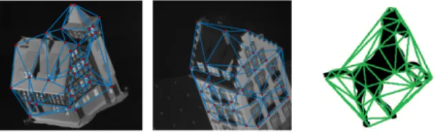
Fig. 5. Examples of HOUSE-HOTEL (Left) and HORSE (Right) database instances.

5. Experiments

This section aims to experimentally evaluate our model. For this, we have conducted experiments using five different datasets. The section is divided as follows, in 5.1 we describe the datasets used in the experiments, in 5.2, we show the performance of our

model when computing the cost matrix using different methods to estimate the costs, in 5.3, we compare its performance in terms of matching accuracy with respect to the best state-of-the-art results. Finally, in 5.4, we study the computational cost of our model.

5.1. Databases

We have used five datasets from two commonly used databases, described in detail in (Moreno-Garc´ıa and Francesc, 2016). The

particularity of this datasests is that they have the ground-truth correspondence between nodes. This information is necessary to

train and experimentally validate the model we present. The first pair of datasets belongs to the HOUSE-HOTEL database (Figure

5, left). Each dataset has two frame sequences corresponding to two different computer modelled objects, a House (111 frames) and a Hotel (101 frames). The objects change position (translation and rotation) throughout the video. Each frame has 30 salient

points.

The Horse database (Figure 5, right), is based on an original drawing from (Alexander M., 2009). In this case, each dataset

has 199 elements artificially generated applying three different kinds of distortions (NOISE, ROTATION, SHEAR) to the original image. In this case, each image has 35 identified salient points.

The graphs was build using the salient points as nodes, each salient point has 60 Context Shape features and and the structure

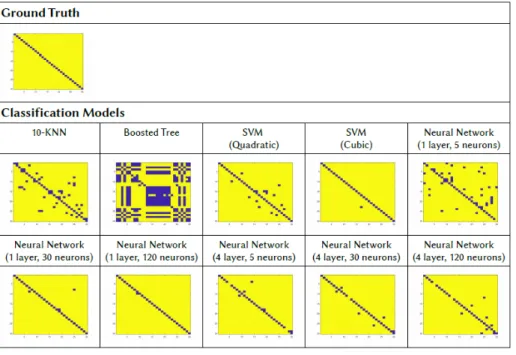
Fig. 6. Cost matrix heatmaps between two graphs corresponding to the HOTEL dataset (90 frames of separation) using different costs estimation models based on binary classifiers. Blue color represents low costs values while yellow color represents high costs.

5.2. Cost Matrix

The purpose of this experiment is to visually compare differences of performance between different ML models estimating edit costs. We show the heatmaps of the resultant cost matrix (M matrix in Algorithm 1) using different cost estimation models based on our framework. In this case, the aim of our model is to find a cost matrix that minimizes the costs when a pair of nodes should

be mapped according to the ground-truth correspondence and maximizing the costs when not. Since we know the ground-truth

correspondence and the nodes are labeled, we can deduce the ground-truth cost matrix. For this experiment, we choose the first pair

of graphs in the test set of the HOTEL sequence separated by 90 frames and the model has been trained with all the graphs in the

training set separated by the same number of frames.

Figure 6 shows the results using different binary classifiers to estimate the edit costs. These models are based on classifying if the cost of an edit operation between a pair of nodes is zero or one. There are no intermediate values between zero and one, since

the output of the model is a discrete class. We can see that the models that perform better in this case are those based on Neural

Networks (Schmidhuber, 2015) or Support Vector Machines for binary classification (Cortes, 1995), while KNN and Boosted Trees

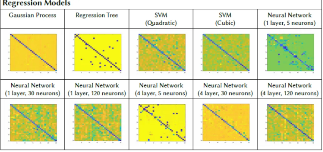
Fig. 7. Cost matrix heatmaps between two graphs corresponding to the HOTEL dataset (90 frames of separation) using different cost estimation models based on regression analysis. Blue color represents low costs values while yellow color represents high costs.

Figure 7 shows the results using models based on parameters regression to estimate the edit costs. These models try to

statis-tically find the relationships among the given input variables and the expected output values by regression analysis. In this case,

the output is defined within a range of continuous values. We train the model providing as the expected outputs, zeros or ones,

according to the criteria defined in 4.2. The resulting cost matrix is more informative in this case since each cell can take a wide

range of values. Regression Trees (?) tends to take values close to extremes which may affect its performance negatively while

Gaussians Process (?) it seems that performs slightly better than Neural Netwroks or Support Vectors Machines for parameters

regression (Drucker, 1996).

Finally and to illustrate the performance of our framework, in Figure 8, we show an example of correspondences found when

costs have been estimated through four different cost estimation models.

Fig. 8. Correspondences found between two graphs of the HOTEL sequence by our framework using four different ML algorithms to estimate the costs. Blue lines are the edges between nodes. Green lines: correct correspondences. Red lines: wrong correspondences.

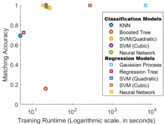
Fig. 9. Matching Accuracy versus Runtime (training the model).

5.3. Matching Accuracy

The main goal of our framework is to learn edit cost estimation models such that we maximize the graph matching accuracy.

Namely, the number of to-node mappings in the correspondence found by the GED (Algorithm 1) that are equal to the

node-to-node mappings of the ground-truth correspondence, normalized by the graphs order.

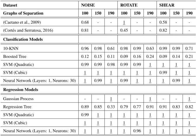
In the following experiment we show the matching accuracy results achieved by different cost estimation models based on our framework. Table 2 shows the results for the HOUSE and HOTEL datasets while Table 3 the results for the NOISE, ROTATE and

SHEAR datasets. The baseline for both experiments is the number of graphs of separation in the dataset. The more separated are

two graphs, the more different they are and consequently, the matching process should be more difficult. We compare our results with the methods presented in (Caetano et al., 2009) and (Cort´es and Serratosa, 2016).

Generally, methods based on regression models tend to perform better than those that classify costs. Apparently it is because,

as we have seen in section 5.2, these methods provide a matrix with more information to the solver. However, there are no big

differences between these approaches when we use Vector Support Machines or Neural Networks and in both cases they overcome the state-of-the-art widely. On the other hand, KNN, Boosted Trees and Regression Trees work worse. The Gaussian Process works

well in the evaluated cases, however, due to its excessive computational complexityO(n3) when training the model (?), we have not

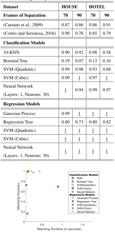
Table 2. Matching accuracy results on HOUSE and HOTEL datasets.

Dataset HOUSE HOTEL Frames of Separation 70 90 70 90

(Caetano et al., 2009) 0.87 0.86 0.86 0.91 (Cort´es and Serratosa, 2016) 0.90 0.76 0.85 0.79

Classification Models 10-KNN 0.90 0.92 0.98 0.58 Boosted Tree 0.19 0.07 0.13 0.16 SVM (Quadratic) 0.99 0.98 0.93 0.88 SVM (Cubic) 0.99 1 0.97 1 Neural Network (Layers: 1, Neurons: 30) 1 0.94 0.99 0.97 Regression Models Gaussian Process 0.99 1 1 1 Regression Tree 0.80 0.73 0.80 0.82 SVM (Quadratic) 1 1 1 1 SVM (Cubic) 1 1 1 1 Neural Network (Layers: 1, Neurons: 30) 1 1 1 1

Fig. 10. Matching Accuracy versus Runtime (computing GED).

5.4. Computational Cost Analysis

One of the main requirements in pattern recognition is to have the ability to perform tasks as fast as possible. In this section we

will evaluate the performance of the different models proposed in the experiments in terms of computational cost. For this, we have studied the computational cost of our model during the training phase and performing the graph matching. The values correspond to

Table 3. Matching accuracy results on NOISE, ROTATE and SHEAR datasets.

Dataset NOISE ROTATE SHEAR

Graphs of Separation 100 150 190 100 150 190 100 150 190

(Caetano et al., 2009) 0.68 - - 1 - - 0.58 -

-(Cort´es and Serratosa, 2016) 0.81 - - 0.45 - - 0.82 -

-Classification Models

10-KNN 0.96 0.98 0.61 0.98 0.99 0.63 0.99 0.99 0.71

Boosted Tree 0.12 0.15 0.11 0.09 0.16 0.24 0.09 0.14 0.21

SVM (Quadratic) 0.99 0.99 0.98 0.99 0.99 1 1 1 1

SVM (Cubic) 1 1 1 1 1 1 0.99 1 1

Neural Network (Layers: 1, Neurons: 30) 1 0.99 1 0.99 1 1 1 0.99 1

Regression Models

Gaussian Process - - 1 - - 1 - - 1

Regression Tree 0.89 0.85 0.33 0.79 0.77 0.91 0.91 0.83 0.82

SVM (Quadratic) 0.99 1 1 1 1 1 1 1 1

SVM (Cubic) 1 1 1 1 1 1 1 1 1

Neural Network (Layers: 1, Neurons: 30) 1 1 1 1 0.96 1 1 1 1

the average results of the experiments performed before with 90 frames of separation for HOUSE and HOTEL and 190 for NOISE,

ROTATE and SHEAR.

Figure 9 shows the mean matching accuracy with respect the mean runtime spent to train the model. Despite its good

perfor-mance in terms of matching accuracy, the Gaussian Process presents serious scalability problems when the size of the training set

is large. On the other hand, KNN does not require training time, however its performance in terms of accuracy is far from the best

models. The best balanced models in our experiments in terms of training cost, are the SVM (Quadratic and Cubic) based on binary

classifiers and Neural Networks, regardless of whether they are based, on regression or classification.

Finally, Figure 10 shows the mean matching accuracy with respect the mean runtime spent when computing the GED. As

expected, the slowest model is the KNN. It also has scalability problems since it has to perform as many operations as labeled

elements are in the training set. The models based on trees are the fastest, but their performance in terms of matching accuracy is

6. Conclusion

We have presented a general framework to learn edit costs for Graphs Edit Distance. In the experiments we have evaluated

different ML algorithms on our framework in terms of matching accuracy and computational cost, proving its versatility. Many of the algorithms experimentally evaluated, can overcome, with a wide margin, the results of the current state-of-the-art. This means

that they can manage important distortions in the representations when they try to estimate the best correspondence because they

are able to take advantage of the ability of ML algorithms to learn correlations between node attributes instead of having to define

the cost functionsa prioriwhen we want to estimate the costs of the edit operations.

However, the performance of the different models present some variations depending on the ML algorithm. The models based on decision trees, such as the Boosted Trees or Regression Trees, are the ones that work worse since they focus on the runtime

efficiency over accuracy. The KNN is a non-parametric classification method that has problems capturing statistical variation when the number of labeled matchings is small and does not scale correctly when it increases since it has to make as many operations

as elements are in the training set. Gaussian Process is a powerful non-linear multivariate interpolation tool successfully used for

parameters regression. In our experiments performs very well in terms of matching accuracy, however, the training algorithm of

this model has a high computational cost.

We also conducted some experiments using cubic and quadratic Support Vector Machines. These models are able to find

non-linear correlations between the attributes of the nodes performing classification or parameters regression. The results with these

models are very good, both in terms of matching accuracy and runtime.

Finally, Neural Networks deserve special attention in their behavior, we observe how these models tend to perform better

when we increase the complexity of the network (number of neurons and layers) until reaching a point where there is no more

improvement. This can be explained because when we increase the network complexity, the model is able to find deeper non-linear

correlations between the attributes that feature the nodes, but reached a critical point, there are more neurons than the ones that can

be justified by the complexity of the input data. In general, they perform very well in the experiments.

be trained. In the future it would be interesting to explore new models to embed node-to-node assignments as well as to evaluate

its performance with other ML algorithms. Also we plan to conduct a more theoretical analysis on the impact of different ML algorithms on the problem in hand. Finally it would be interesting to expand the model including insertions and deletions costs.

References

Alexander M., Bronstein M., B.A.M.B.R., 2009. Partial similarity of objects, or how to compare a centaur to a horse. International Journal of Computer Vision 84, 163–183.

Bunke H., A.G., 1983. Inexact graph matching for structural pattern recognition. Pattern Recognition Letters 4, 245–253.

Caetano, T.S., McAuley, J.J., Cheng, L., Le, Q.V., Smola, A.J., 2009. Learning graph matching. IEEE transactions on pattern analysis and machine intelligence 31, 1048–1058.

Conte, D., Foggia, P., Sansone, C., Vento, M., 2004. Thirty years of graph matching in pattern recognition. International journal of pattern recognition and artificial intelligence 18, 265–298.

Cortes, C., 1995. Support-vector networks. Machine Learning 20, 273–297.

Cort´es, X., Conte, D., Cardot, H., Serratosa, F., 2018. A deep neural network architecture to estimate node assignment costs for the graph edit distance. Syntactic and Structural Pattern Recognition , 326–336.

Cort´es, X., Serratosa, F., 2015. Learning graph-matching edit-costs based on the optimality of the oracle’s node correspondences. Pattern Recognition Letters 56, 22–29.

Cort´es, X., Serratosa, F., 2016. Learning graph matching substitution weights based on the ground truth node correspondence. International Journal of Pattern Recognition and Artificial Intelligence 30, 1650005.

Drucker, H., B.C.J.C.K.L.S.A.J.V.V.N., 1996. Support vector regression machines. Advances in Neural Information Processing Systems (NIPS) , 155161. Hastie, T.; Tibshirani, R.F.J.H., 2009. Boosting and additive trees. The Elements of Statistical Learning , 337–384.

Kuhn, H.W., 1955. The hungarian method for the assignment problem. Naval Research Logistics Quarterly 2, 83–97.

Leordeanu, M., Sukthankar, R., Hebert, M., 2012. Unsupervised learning for graph matching. International journal of computer vision 96, 28–45.

Moreno-Garc´ıa, Carlos Francisco, C.X., Francesc, S., 2016. A graph repository for learning error-tolerant graph matching. Syntactic and Structural Pattern Recognition .

Neuhaus, M., Bunke, H., 2005. Self-organizing maps for learning the edit costs in graph matching. IEEE Transactions on Systems, Man, and Cybernetics, Part B (Cybernetics) 35, 503–514.

Neuhaus, M., Bunke, H., 2007. Automatic learning of cost functions for graph edit distance. Information Sciences 177, 239–247.

Raveaux R., Martineau M., C.D.V.G., 2017. Learning graph matching with a graph-based perceptron in a classification context. GbRPR 2017 , 49–58. Riesen, K., Bunke, H., 2009. Approximate graph edit distance computation by means of bipartite graph matching. Image and Vision computing 27, 950–959. Riesen K., F.M., 2016. Predicting the correctness of node assignments in bipartite graph matching. Pattern Recognition Letters 69, 8–14.

Schmidhuber, J., 2015. Deep learning in neural networks: An overview. Neural Networks 61, 85–117.

Serratosa, F., Cort´es, X., 2015. Graph edit distance: Moving from global to local structure to solve the graph-matching problem. Pattern Recognition Letters 65, 204–210.