Diversity in Ensemble Feature Selection

Diversity in Ensemble Feature Selection

Alexey Tsymbala*, Mykola Pechenizkiyb, Pádraig Cunninghama

a

Department of Computer Science, Trinity College Dublin, Ireland Alexey.Tsymbal@cs.tcd.ie, Padraig.Cunningham@cs.tcd.ie

*

tel.: +353-1-6083837; fax: +353-1-6772204

b

Department of Computer Science and Information Systems, University of Jyväskylä, Finland

mpechen@cs.jyu.fi

Diversity in Ensemble Feature Selection

Abstract

Ensembles of learnt models constitute one of the main current directions in machine learning and data mining. Ensembles allow us to achieve higher accuracy, which is often not achievable with single models. It was shown theoretically and experimentally that in order for an ensemble to be effective, it should consist of high-accuracy base classifiers that should have high diversity in their predictions. One technique, which proved to be effective for constructing an ensemble of accurate and diverse base classifiers, is to use different feature subsets, or so-called ensemble feature selection. Many ensemble feature selection strategies incorporate diversity as a component of the fitness function in the search for the best collection of feature subsets. There are known a number of ways to quantify diversity in ensembles of classifiers, and little research has been done about their appropriateness to ensemble feature selection. In this paper, we compare seven measures of diversity with regard to their possible use in ensemble feature selection. We conduct experiments on 21 data sets from the UCI machine learning repository, comparing the ensemble accuracy and other characteristics for the ensembles built with ensemble feature selection based on the considered measures of diversity. We consider five search strategies for ensemble feature selection: simple random subsampling, genetic search, hill-climbing, ensemble forward and backward sequential selection. In the experiments, we show that, in some cases, the ensemble feature selection process can be sensitive to the choice of the diversity measure, and that the question of the superiority of a particular measure depends on the context of the use of diversity and on the data being processed.

Keywords: Ensemble of classifiers; Ensemble diversity; Feature selection; Search strategy; Dynamic

integration of classifiers

1 Introduction

Current electronic data repositories are growing quickly and contain a huge amount of data from commercial, scientific, and other domain areas. This data includes also currently unknown and potentially interesting patterns and relations, which can be uncovered using knowledge discovery and data mining methods [13].

improve classification results, is currently an active research area in the machine learning and neural networks communities [2, 4 – 11, 14 – 17, 20 – 31, 34 – 43]. Dietterich [10] has presented the integration of multiple classifiers as one of the four most important directions in the machine learning research. It was shown in many domains that an ensemble is often more accurate than any of the single classifiers in the ensemble.

Both theoretical and empirical research have demonstrated that a good ensemble is one where the base classifiers in the ensemble are both accurate and tend to err in different parts of the instance space (that is have high diversity in their predictions). Another important issue in creating an effective ensemble is the choice of the function for combining the predictions of the base classifiers. It was shown that increasing coverage of an ensemble through diversity is not enough to ensure increased prediction accuracy – if the integration method does not utilize coverage, then no benefit arises from integrating multiple models [4].

One effective approach for generating an ensemble of accurate and diverse base classifiers is to use different feature subsets, or so-called ensemble feature selection [27]. By varying the feature subsets used to generate the base classifiers, it is possible to promote diversity and produce base classifiers that tend to err in different subareas of the instance space. While traditional feature selection algorithms have the goal of finding the best feature subset that is relevant to both the learning task and the selected inductive learning algorithm, the task of ensemble feature selection has the additional goal of finding a set of feature subsets that will promote disagreement among the base classifiers [27].

Ho [17] has shown that simple random selection of feature subsets may be an effective technique for ensemble feature selection because the lack of accuracy in the ensemble members is compensated for by their diversity. Random subspacing is used as a base in a number of ensemble feature selection strategies, e.g. GEFS [27] and HC [8].

Feature selection algorithms, including ensemble feature selection, are typically composed of the following components [1, 27]: (1) search strategy, that searches the space of feature subsets; and (2)

fitness function, that inputs a feature subset and outputs a numeric evaluation. The search strategy’s

goal is to find a feature subset maximizing this function.

As it is acknowledged that an effective ensemble should consist of high-accuracy classifiers that disagree on their predictions, many fitness functions in ensemble feature selection include explicitly or implicitly both accuracy and diversity. One measure of fitness, which was proposed by Opitz [27], defines the fitness Fitnessi of a classifier i corresponding to a feature subset i to be proportional to the

classifier i to the total ensemble diversity, which can be measured as the average pairwise diversity for all the pairs of classifiers including i):

i i

i acc div

Fitness = +α⋅ , (1)

where α is the coefficient of the degree of the influence of diversity. This fitness function was also used in experiments in [39], and we use it in our experiments in this paper.

A common measure of classification accuracy is the percentage of correct classifications on the test data set, or average within-class accuracy, the average percentage of correct classifications within each class, if the class distributions are significantly uneven. The simple “percentage of correct classifications” measure is successfully used in the vast majority of cases, as it reflects well the classification performance. For diversity, the situation is not that straightforward – there are known a number of ways to measure diversity in ensembles of classifiers, and not much research has been done about the appropriateness and superiority of one measure over another.

In this paper, we consider different measures of ensemble diversity, which could be used as a component of the fitness function (1), and which could also be used to measure total ensemble diversity, as a general characteristic of ensemble goodness. The goal of this paper is to compare the considered measures of diversity in the context of ensemble feature selection for these two particular tasks. To our knowledge, in all the existent research papers, comparing different measures of ensemble diversity, as [22, 34], the only common way of the comparison is to analyze the correlation of those measures of diversity with different other ensemble characteristic, as the ensemble accuracy, the difference between the ensemble accuracy and the average base classifier accuracy, the difference between the ensemble accuracy and the maximal base classifier accuracy, etc. In contrast to that common way, in this paper we compare the measures of diversity using the wrapper approach, applying them as a component of the fitness function guiding the search in ensemble feature selection, and comparing the resulting accuracies and other ensemble characteristics.

2 An ensemble and its diversity

In this section, we consider: the question of what constitutes a good ensemble, effective techniques for generating the base classifiers in ensembles, the place of ensemble feature selection among them, and search strategies for ensemble feature selection, which we shall use in our experiments.

2.1 Ensemble goodness criteria and their interrelation

An ensemble is generally more accurate than any of the base classifiers in the ensemble. Both theoretical and empirical research have shown that an effective ensemble should consist of base classifiers that not only have high classification accuracy, but that also make their errors in different parts of the input space [4, 9, 15, 21, 41]. Brodley and Lane [4] show that the main objective when generating the base classifiers is to maximize the coverage on the data, which is the percentage of the instances that at least one base classifier can classify correctly. Achieving coverage greater than the accuracy of the best base classifier requires diversity among the base classifiers. Several researchers have presented theoretical evidence supporting this claim [15, 21, 41].

For example, Hansen and Salamon [15] proved that, if the average classification error rate for an instance is less than 50% and the base classifiers in the ensemble are independent in the production of their errors, then the expected error for that instance can be reduced to zero as the number of base classifiers included into the ensemble goes to infinity, when majority voting is used for integration. Such assumptions rarely hold in practice (for example, an outlier may easily have predicted classification error rate that is higher than 50%), and then the classification error rate over all the instances cannot necessarily be reduced to zero. But if we assume a significant percentage of the instances are predicted with less than 50% average error, gains in generalization will be achieved. A key assumption in this analysis is that the base classifiers should be independent in their production of errors.

Krogh and Vedelsby [21] have shown that the classification error for an ensemble of neural network base predictors is related to the generalization error of the base networks and to how much disagreement there is between them. They have proved that E=E−A, where E is the ensemble

generalization error, E is the average of the generalization errors of the base networks weighted by

A similar dependency derived by Tumer and Ghosh [41] for classifiers that predict the a posteriori probabilities of the output classes is:

E S

P S

E

L

i i i

⋅ ⋅

− +

=

∑

) 1 (

1 δ

, (2)

where E is the ensemble generalization error (beyond the optimal Bayesian error), S is the size of the ensemble, Pi is the prior probability of class i, δ_i is the average correlation factor among the

classifiers in the prediction of the a posteriori probabilities of class i, and E is the average error of the

base classifier. Here the disagreement is measured as the correlation in the predictions of the a posteriori probabilities.

While these theoretical results hold true for regression systems and classifiers that predict a posteriori probabilities, no similar dependencies are known for the more common case of classifiers with crisp predictions, which is the focus of the paper. However, there are a number of approaches to quantify ensemble diversity for the case of crisp classification, which we consider in Section 4.

2.2 Techniques for the generation of base classifiers in ensembles

The task of using an ensemble of models can be broken down into two basic questions: (1) what set of learned models should be generated?; and (2) how should the predictions of the learned models be integrated? [24]. To generate a set of accurate and diverse learned models, several approaches have been tried.

One way of generating a diverse set of models is to use learning algorithms with heterogeneous representations and search biases [24], such as decision trees, neural networks, instance-based learning, etc.

Another approach is to use models with homogeneous representations that differ in their method of search or in the data on which they are trained. This approach includes several techniques for generating base models, such as learning base models from different subsets of the training data. For example, two well-known ensemble methods of this type are bagging and boosting [31].

each bit in the output code. An instance is classified by predicting each bit of its output code (i.e., label), and then classifying the instance as the label with the “closest” matching output code.

Also, natural randomisation in the process of model search (e.g., random weight setting in the backpropagation algorithm for training neural networks) can be used to build different models with homogeneous representation. The randomisation can also be injected artificially. For example, in [16] a randomised decision tree induction algorithm, which generates different decision trees every time it is run, was used for that purpose.

Another way for building models with homogeneous representations, which proved to be effective, is the use of different subsets of features for each model. For example, in [29] base classifiers are built on different feature subsets, where each feature subset includes features relevant for distinguishing one class label from the others (the number of base classifiers is equal to the number of classes). Finding a set of feature subsets for constructing an ensemble of accurate and diverse base models is also known as ensemble feature selection [27].

Sometimes, a combination of the techniques considered above can be useful in order to provide the desired characteristics of the generated models. For example, a combination of boosting and wagging (which is a kind of bagging technique) is considered by Webb [42].

In addition to these general-purpose methods for generating a diverse ensemble of models, there are learning algorithm-specific techniques. For example, Opitz and Shavlik [28] employ a genetic algorithm in backpropagation to search for a good population of neural network classifiers.

Ensemble feature selection is the focus of this paper, and in next section we consider search strategies used in our experiments.

2.3 Search strategies for ensemble feature selection

In this section, we consider four different search strategies for ensemble feature selection: (1) Hill Climbing (HC); (2) a Genetic Algorithm for ensemble feature selection (GA); (3) Ensemble Forward Sequential Selection (EFSS); and (4) Ensemble Backward Sequential Selection (EBSS).

refinement is based on a hill-climbing search. For all the feature subsets, an attempt is made to switch (include or delete) each feature. If the resulting feature subset produces better performance on the validation set (the fitness function returns a better value for it), that change is kept. This process is continued until no further improvements are possible. Normally, no more than 4 passes are necessary.

The use of genetic search has also been an important direction in the feature selection research. Genetic algorithms have been shown to be effective global optimization techniques in feature subset selection. The use of genetic algorithms for ensemble feature selection was first proposed in [27]. The Genetic Algorithm for ensemble feature selection (GA) strategy [27] begins, as HC, with creating an initial population of classifiers where each classifier is generated by randomly selecting a different subset of features. Then, new candidate classifiers are continually produced by using the genetic operators of crossover and mutation on the feature subsets. After producing a certain number of individuals the process continues with selecting a new subset of candidates by selecting the members randomly with a probability proportional to fitness (it is known as roulette-wheel selection). The process of producing new classifiers and selecting a subset of them (a generation) continues a number of times, known as the number of generations. After a predefined number of generations, the fittest individuals make up the population, which comprises the ensemble [27]. In our implementation, the representation of each individual (a feature subset) is simply a constant-length string of bits, where each bit corresponds to a particular feature. The crossover operator uses uniform crossover, in which each feature of the two children takes randomly a value from one of the parents. The feature subsets of two individuals in the current population are chosen randomly with a probability proportional to (1+fitness). The mutation operator randomly toggles a percentage of bits in an individual.

EFSS and EBSS are sequential feature selection strategies, which add or delete features using a hill-climbing procedure, and have polynomial complexity. The most frequently studied variants of plain sequential feature selections algorithms (which select a single feature subset) are forward and backward sequential selection, FSS and BSS [1]. FSS begins with zero attributes, evaluates all feature subsets with exactly one feature, and selects the one with the best performance. It then adds to this subset the feature that yields the best performance for subsets of the next larger size. The cycle repeats until no improvement is obtained from extending the current subset. BSS instead begins with all features and repeatedly removes a feature whose removal yields the maximal performance improvement [1]. EFSS and EBSS iteratively apply FSS or BSS to form each of the base classifiers using a predefined fitness function.

features included or deleted on average in an FSS or BSS search. HC has similar polynomial complexity O(S⋅F⋅N_passes), where N_passes is the average number of passes through the feature subsets in HC until there is some improvement (usually no more than 4). The complexity of GEFS does not depend on the number of features, and is O(S ⋅′N_gen), where S′ is the number of individuals (feature subsets) in one generation, and N_gen is the number of generations.

In our experiments, on average, each of the strategies looks through about 1000 feature subsets (given that the number of base classifiers is 25, the average number of features is 10, the average percentage included or deleted features in EFSS and EBSS is 40%, the number of passes in HC is 4, the number of individuals in a population in the GA is 100, and the number of generations is 10).

Comparative experiments with these four strategies on a collection of data sets from the medical field of acute abdominal pain classification were considered in [38]. The best search strategy in that context was EFSS (it was the best for every data set considered), generating more diverse ensembles with more compact base classifiers. EFSS generated extremely compact base classifiers, including from 9% to 13% features on average (less than 3 features). The results with genetic search were found to be disappointing, not being improved with generations.

In comparison with [38] we have made a number of changes in the genetic search-based strategy. In our new version considered in this paper no full feature sets are allowed in random subspacing nor may the crossover operator produce a full feature subset. Individuals for crossover are selected randomly proportional to log(1+fitness) instead of just fitness, which adds more diversity into the new population. The generation of children identical to their parents is prohibited in the crossover operator – if a child is the same as one of its parents, the mutation operator is applied to it. To provide a better diversity in the length of the feature subsets and the population in general, we use two different mutation operators, one of which always adds features randomly with a given probability, and the other – deletes features. Each operator is applied to exactly a half (25 of 50) of the individuals being mutated. Our pilot studies have shown that these minor changes help us to significantly improve the work of GA so that it does not converge after a single generation already to a local extremum (as it was in [27, 38]).

3 Techniques for integration of an ensemble of models

Brodley and Lane [4] have shown that simply increasing coverage of an ensemble through diversity is not enough to insure increased prediction accuracy. If the integration method does not utilize the coverage, then no benefit arises from integrating multiple classifiers. Thus, the diversity and coverage of an ensemble are not in themselves sufficient conditions for ensemble accuracy. It is also important for ensemble accuracy to have a good integration method that will utilize the diversity of the base models.

The challenging problem of integration is to decide which one(s) of the classifiers to rely on or how to combine the results produced by the base classifiers. Techniques using two basic approaches have been suggested as a solution to the integration problem: (1) a combination approach, where the base classifiers produce their classifications and the final classification is composed using them; and (2) a

selection approach, where one of the classifiers is selected and the final classification is the result

produced by it.

Several effective techniques for the combination of classifiers have been proposed. One of the most popular and simplest techniques used to combine the results of the base classifiers, is simple voting (also called majority voting and select all majority (SAM)) [2]. In the voting technique, the classification of each base classifier is considered as an equally weighted vote for that particular classification. The classification that receives the biggest number of votes is selected as the final classification (ties are solved arbitrarily). Often, weighted voting is used: each vote receives a weight, which is usually proportional to the estimated generalization performance of the corresponding classifier. Weighted Voting (WV) works usually much better than simple majority voting [2].

More sophisticated combination techniques include the SCANN method based on the correspondence analysis and using the nearest neighbor search in the correspondence analysis results [24, 26]; and techniques to combine minimal nearest neighbor classifiers within the stacked generalization framework [35]. Two effective classifier combination techniques based on stacked generalization called “arbiter” and “combiner” were presented by Chan [5]. Hierarchical classifier combination has also been considered. Experimental results of Chan and Stolfo [5, 6] showed that the hierarchical (multi-level) combination approach, where the dataset was distributed among a number of sites, was often able to sustain the same level of accuracy as a global classifier trained on the entire dataset.

base classifier is estimated using the training set, and then the classifier with the highest accuracy is selected (ties are solved using voting). More sophisticated selection approaches include estimation of the local accuracy of the base classifiers by considering errors made in instances with similar predictions [25], learning a number of meta-level classifiers (“ referees” ) that predict whether the corresponding base classifiers are correct or not for new instances (each “ referee” is a C4.5 tree that recognizes two classes) [20]. Todorovski and Dzeroski [37] trained a meta-level decision tree, which dynamically selected a base model to be applied to the considered instance, using the level of confidence of the base models in correctly classifying the instance.

The approaches to classifier selection can be divided into two subsets: static and dynamic selection. The static approaches propose one “ best” method for the whole data space, while the dynamic approaches take into account each new instance to be classified and its neighbourhood only. The CVM is an example of the static approach, while the other selection techniques considered above are examples of the dynamic approach.

Techniques for combining classifiers can be static or dynamic as well. For example, widely used weighted voting [2] is a static approach. The weights for each base classifier’s vote do not depend on the instance to be classified. In contrast, the reliability-based weighted voting (RBWV) introduced in [7] is a dynamic voting approach. It uses classifier-dependent estimation of the reliability of predictions for each particular instance. Usually, better results can be achieved if the classifier integration is done dynamically taking into account the characteristics of each new instance.

We consider in our experiments three dynamic approaches based on the local accuracy estimates: Dynamic Selection (DS) [30], Dynamic Voting (DV) [30], and Dynamic Voting with Selection (DVS) [40]. All these are based on the same local accuracy estimates. DS simply selects a classifier with the least predicted local classification error, as was also proposed in [14]. In DV, each base classifier receives a weight that is proportional to the estimated local accuracy of the base classifier, and the final classification is produced by combining the votes of each classifier with their weights. In DVS, the base classifiers with highest local classification errors are discarded (the classifiers with errors that fall into the upper half of the error interval of the base classifiers) and locally weighted voting (DV) is applied to the remaining base classifiers.

4 Diversities

classifier pairs in the ensemble (plain disagreement, fail/non-fail disagreement, the Q statistic, the correlation coefficient, and the kappa statistic), and the other two are non-pairwise as they measure diversity in predictions of the whole ensemble only (entropy and ambiguity). In our experiments in this paper, we compare the use of the pairwise measures as the guiding diversity in the ensemble training process (as a component of the fitness function (1)), and consider the correlation of the total average ensemble diversity for all the seven measures with the difference between the ensemble accuracy and the average base classifier accuracy.

4.1 The plain disagreement measure

The plain disagreement measure of diversity is, probably, the most commonly used measure for diversity in the ensembles of classifiers with crisp predictions. For example, in [17] it was used for measuring the diversity of decision forests, and its correlation with the forests’ accuracy. In [39, 43] it was used as a component of the fitness function guiding the process of ensemble construction.

For two classifiers i and j, the plain disagreement is equal to the ratio between the number of instances on which the classifiers make different predictions, to the total number of instances in question:

∑

x , (3)

where N is the number of instances in the data set, C_i(x_k) is the class assigned by classifier i to instance k, and Diff(a,b)=0, if a=b, otherwise Diff(a,b)=1.

The plain disagreement varies from 0 to 1. This measure is equal to 0, when the classifiers return the same classes for each instance, and it is equal to 1 when the predictions are always different.

4.2 The fail/non-fail disagreement measure

The fail/non-fail disagreement was defined in [36] as the percentage of test instances for which the classifiers make different predictions but for which one of them is correct:

00 01 10 11 10 01 _ N N N N N N dis div _i,j + + + +

= , (4)

number of classes is 2. It can be also shown that div_dis_i,j ≤div_plain_i,j, as the instances contributing to this disagreement measure form a subset of instances contributing to the plain disagreement.

The fail/non-fail disagreement varies from 0 to 1. This measure is equal to 0, when the classifiers return the same classes for each instance, or different but incorrect classes, and it is equal to 1 when the predictions are always different and one of them is correct.

4.3 The Q statistic

This measure is based on Yule’s Q statistic used to assess the similarity of two classifiers’ outputs [22]:

10 01 00 11

10 01 00 11

_

N N N N

N N N N Q div _i,j

+ −

= , (5)

where Nab has the same meaning as in (4). For statistically independent classifiers, the expected value of Q is 0. Q varies between –1 and 1. Classifiers that tend to recognize the same objects correctly will have positive values of Q, and those which commit errors on different objects will render Q negative [22]. In the case of undefined value with division by zero, we assume the diversity is minimal, equal to 1.

In our experiments with diversity as a component of the fitness function we normalize this measure to vary from 0 to 1, where 1 corresponds to the maximum of diversity:

2 _ 1

_Q* div Q

div = − . (6)

In [22], after comparative experiments on the UCI Breast cancer Wisconsin data set, the Phoneme recognition and the Cone-torus data sets, and two experiments with emulated ensembles (artificially generating possible cases of the base classifiers’ outputs), Q was recommended as the best measure for the purposes of developing committees that minimize error, taking into account the experimental results, its simplicity and comprehensibility (or the ease of interpretation). In our experiments, we show that the question of the superiority of a particular measure depends on the context of the use of diversity, and on the data being processed.

4.4 The correlation coefficient

The correlation between the outputs of two classifiers i and j can be measured as [22]:

) )( )( )( ( _ 00 10 01 11 00 01 10 11 10 01 00 11 N N N N N N N N N N N N corr div _i,j + + + + −

= , (7)

where Nab have the same meaning as in (4) and (5).

The numerator in (7) is the same as in (5), and for any two classifiers i and j, div_corri,j and div_Qi,j

have the same sign, and it can be proven that div_corr_i,j ≤ div_Q_i,j [22]. We normalize this measure to vary from 0 to 1 in the same way we do it for Q (5).

This measure, as well as the fail/non-fail disagreement and the Q statistic were considered among the group of 10 measures in the comparative experiments in [22].

4.5 The kappa degree-of-agreement statistic

Let Nij be the number of instances in the data set, recognized as class i by the first classifier and as

class j by the second one, Ni* is the number of instances recognized as i by the first classifier, and N*i is

the number of instances recognized as iE\WKHVHFRQGFODVVLILHU'HILQHWKHQ 1DQG 2 as

N N l i ii

∑

1 , and

∑

=     _⋅ = Θ l i N N N N_{i i}

1

2 * * , (8)

ZKHUH1LVWKHWRWDOQXPEHURILQVWDQFHV 1 estimates the probability that the two classifiers agree, and 2LVDFRUUHFWLRQWHUPIRU 1, which estimates the probability that the two classifiers agree simply by

chance (in the case where each classifier chooses to assign a class label randomly). The pairwise diversity div_kappai,j is defined as follows [9]:

2 2 1 1 _ Θ − Θ − Θ = i,j kappa

div . (9)

Kappa is equal to 0 when the agreement of the two classifiers equals to that expected by chance, and

kappa is equal to 1 when the two classifiers agree on every example. Negative values occur when

Dietterich [9] used this measure in scatter plots called “ -error diagrams” , where kappa was plotted against mean accuracy of the classifier pair. -error diagrams, introduced in [23] is a useful tool for visualising ensembles.

4.6 Entropy

A non-pairwise measure of diversity, associated with a conditional-entropy error measure, is based on the concept of entropy [8]:

∑ ∑

= =

      ⋅ −

= N

i l

k S

N S

N_ki _ki

N ent div

1 1

log 1

_ , (10)

where N is the number of instances in the data set, S is the number of base classifiers, l is the number of classes, and N is the number of base classifiers that assign instance i to class k. To keep this measure _ki

of diversity within the range [0,1] the logarithm should be taken to the base l.

This measure was evaluated on a medical prediction problem and was shown to predict the accuracy of the ensemble well [8]. It was also shown that the entropy measure of diversity has the added advantage that it models the change in diversity with the size of the ensemble.

While this may be a useful measure of diversity, it does not allow us to gauge the contribution of an individual classifier to diversity because it is not a pairwise measure [43]. Thus, we shall use this total measure of diversity only in our experiments on the correlation between the total ensemble diversity and the difference in ensemble accuracy and the base classifier accuracy.

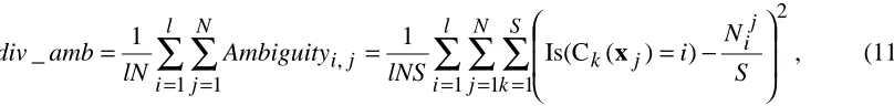
4.7 A variance-based measure: Ambiguity

∑ ∑ ∑

∑ ∑

1 1 1

2

1 1

, Is(C ( ) )

1 1

_ x , (11)

where l is the number of classes, N is the number of instances, S is the number of base classifiers, N _ij

is the number of base classifiers that assign instance j to class i, C_k(x_j) is the class assigned by classifier k to instance j, and Is() is a truth predicate.

As with entropy, this is a non-pairwise measure, and we shall use it only in our experiments on the correlation between the total ensemble diversity and the difference in the ensemble accuracy and the base classifier accuracy.

5 Experimental investigations

In this section, our experiments with the seven measures of diversity in ensemble feature selection are presented. First, the experimental setting is described, then the results of the experiments are presented. The experiments are conducted on 21 data sets taken from the UCI machine learning repository [3]. These data sets include real-world and synthetic problems, vary in characteristics, and were previously investigated by other researchers.

The main characteristics of the 21 data sets are presented in Table 1. The table includes the name of a data set, the number of instances included in the data set, the number of different classes of instances in the data set, and the numbers of different kinds of features included in the instances of the data set.

In [32] the use of the data sets from the UCI repository was strongly criticized. Any new experiments on the UCI data sets run the risk of finding “ significant” results that are no more than statistical accidents. However, we do believe that nevertheless, the UCI data sets provide useful benchmark estimates that can be of great help in experimental analysis and comparisons of learning methods, even though these results must be looked at carefully before final conclusions are made.

Table 1. Data sets and their characteristics

Features Data set Instances Classes

Categorical Numerical

Balance 625 3 0 4

Breast Cancer Ljubljana 286 2 9 0

Car 1728 4 6 0

Pima Indians Diabetes 768 2 0 8

Glass Recognition 214 6 0 9

Heart Disease 270 2 0 13

Ionosphere 351 2 0 34

Iris Plants 150 3 0 4

LED17 300 10 24 0

Liver Disorders 345 2 0 6

Lymphography 148 4 15 3

MONK-1 432 2 6 0

MONK-2 432 2 6 0

MONK-3 432 2 6 0

Soybean 47 4 0 35

Thyroid 215 3 0 5

Tic-Tac-Toe Endgame 958 2 9 0

Vehicle 846 4 0 18

Voting 435 2 16 0

Zoo 101 7 16 0

5.1 Experimental setting

For our experiments, we used an updated version of the setting presented in [39] to test the EFS_SBC algorithm (Ensemble Feature Selection with the Simple Bayesian Classification). We extended the EFS_SBC setting with an implementation of three new search strategies besides the existing HC: GA, EFSS, and EBSS (Section 2.3), and with an implementation of six new measures of diversity besides the existing plain disagreement: the fail/non-fail disagreement, the Q statistic, the correlation coefficient, the kappa statistic, entropy and ambiguity (Section 4).

We used the simple Bayesian classification as the base classifiers in the ensembles. It has been recently shown experimentally and theoretically that the simple Bayes can be optimal even when the “ naïve” feature-independence assumption is violated by a wide margin [12]. Second, when the simple Bayes is applied to the subproblems of lower dimensionalities as in random subspacing, the error bias of the Bayesian probability estimates caused by the feature-independence assumption becomes smaller. It also can easily handle missing feature values of a learning instance allowing the other feature values still to contribute. Besides, it has advantages in terms of simplicity, learning speed, classification speed, and storage space, which made it possible to conduct all the experiments within reasonable time. It was shown [39] that only one “ global” contingency table is needed for the whole ensemble when the simple Bayes is employed in ensemble feature selection. We believe that the results presented in this paper do not depend significantly on the learning algorithm used and would be similar for most known learning algorithms.

class is taken, so that the class distributions of instances in the resulting sets are approximately the same as in the initial data set. It was shown that such sampling often gives better accuracy estimates than simple random sampling [18]. Each time 60 percent of instances are assigned to the training set. The remaining 40 percent of instances of the data set are divided into two sets of approximately equal size (VS and TS). The validation set VS is used in the ensemble refinement to estimate the accuracy and diversity guiding the search process. The test set TS is used for the final estimation of the ensemble accuracy. We have used the same division of the data into the training, validation and test sets for each search strategy and guiding diversity to avoid unnecessary variance and provide better comparison.

The ensemble size S was selected to be 25. It has been shown that for many ensembles, the biggest gain in accuracy is achieved already with this number of base classifiers [2].

We experimented with seven different values of the diversity coefficient α: 0, 0.25, 0.5, 1, 2, 4, and 8. At each run of the algorithm, we collect accuracies for the five types of integration of the base classifiers (Section 3): Static Selection (SS), Weighted Voting (WV), Dynamic Selection (DS), Dynamic Voting (DV), and Dynamic Voting with Selection (DVS). In the dynamic integration strategies DS, DV, and DVS, the number of nearest neighbors (k) for the local accuracy estimates was pre-selected from the set of seven values: 1, 3, 7, 15, 31, 63, 127 (2n −1, n=1,...,7), for each data set separately, if the number of instances in the training set permitted. Such values were chosen, as the nearest-neighbor procedure in the dynamic integration is distance-weighted. The distances from the test instance to the neighboring training instances were computed and used to calculate the estimates of local accuracies. As it was shown in [14], this makes the dynamic integration less sensitive to the choice of the number of neighbors, but still the local accuracy estimates are more sensitive to the small number of neighbors. Heterogeneous Euclidean-Overlap Metric (HEOM) [30] was used for calculation of the distances. In the dynamic integration, we used 10-fold cross validation for building the cross-validation history for the estimation of the local accuracies of the base classifiers.

To select the best α and k, we conducted a separate series of experiments using the wrapper approach for each combination of a search strategy, guiding diversity, integration method, and data set. After, the experiments were repeated with the pre-selected values of α and k.

The test environment was implemented within the MLC++ framework (the machine learning library in C++)[19]. A multiplicative factor of 1 was used for the Laplace correction in simple Bayes as in [12]. Numeric features were discretized into ten equal-length intervals (or one per observed value, whichever was less), as it was done in [12]. Although this approach was found to be slightly less accurate than more sophisticated ones, it has the advantage of simplicity, and is sufficient for comparing different ensembles of simple Bayesian classifiers with each other, and with the “ global” simple Bayesian classifier. The use of more sophisticated discretization approaches could lead to better classification accuracies for the base classifiers and ensembles, but should not influence the results of the comparison.

5.2 Correlation between the total ensemble diversity and the difference between the ensemble

accuracy and the average base classifier accuracy

First, we measured correlation between the total ensemble diversity and the difference between the ensemble accuracy and the average base classifier accuracy. To measure the correlation we used the commonly used Pearson’ s linear correlation coefficient r and a non-parametric counterpart to it - Spearman’ s rank correlation coefficient (RCC).

RCC is a nonparametric (distribution-free) rank statistic proposed by Spearman in 1904 as a measure

of the strength of the associations between two variables. It is a measure of monotone association that is used when the distribution of the data make Pearson's correlation coefficient undesirable or misleading. Kuncheva and Whitaker [22] have used RCC in similar experiments, motivating the choice by the fact that the relationships were not linear. RCC is based on the difference in ranks of the corresponding variables x and y (N here is the number of observations):

∑

= −

− ⋅

−

= N

i

i i

N N

y Rank x

Rank RCC

1 2

2

) 1 (

)) ( )

( ( 6

1 . (12)

In our case, N is equal to 70, corresponding to 70 different measures of the total ensemble diversity and the difference in the ensemble accuracy and the average base classifier accuracy for the 70 cross-validation runs for each data set. We have measured these correlations for the four search strategies, EBSS, EFSS, GA, and HC, and for simple random subsampling (RS). In the search strategies we have used all the five pairwise measures of diversity considered in Section 4.

coefficients was not more than 0.017 for every data set), so we continue our analysis only for the ensembles built with random subsampling.

In Table 2, Pearson’ s correlation coefficient (r) is presented that quantifies the correlation between the total ensemble diversity and the difference between the ensemble accuracy and the average base classifier accuracy for the ensembles built with random subsampling. All the seven diversity measures (Section 4) are considered, corresponding to different columns of the table: (1) the plain disagreement,

div_plain; (2) the fail/non-fail disagreement, div_dis; (3) the Q statistic, div_Q; (4) the correlation

coefficient, div_corr; (5) the kappa statistic, div_kappa; (6) entropy, div_ent; and (7) ambiguity,

div_amb. We measured the correlations for three integration methods (DVS, which is the strongest of

the dynamic integration methods, Weighted Voting, WV, and plain non-weighted Voting), presented in the lines of the table. Each cell corresponding to a measure of diversity and an integration method contains three values: average, maximal and minimal values of the 21 correlation coefficients, calculated for the 21 data sets. Table 3 has the same structure as Table 2 and presents Spearman’ s rank correlation coefficients (RCC).

Table 2. Pearson’ s correlation coefficient (r) for the total ensemble diversity and the difference between the ensemble accuracy and the average base classifier accuracy (average, maximal and minimal values)

r div_plain div_dis div_Q div_corr div_kappa div_ent div_amb

0.534 0.534 0.383 0.436 0.492 0.527 0.534 0.997 0.994 0.702 0.810 0.991 0.979 0.997 DVS

-0.021 -0.011 -0.121 0.007 -0.163 0.021 -0.021 0.459 0.477 0.380 0.435 0.398 0.462 0.459 0.997 0.994 0.791 0.910 0.991 0.979 0.997 WV

0.074 0.108 -0.019 0.040 -0.206 0.108 0.075 0.363 0.404 0.346 0.382 0.292 0.373 0.362 0.997 0.994 0.791 0.910 0.991 0.979 0.997 Voting

-0.312 -0.312 -0.257 -0.360 -0.369 -0.297 -0.312

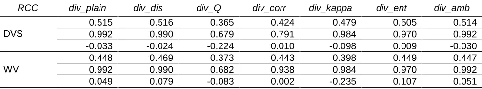
Table 3. Spearman’ s rank correlation coefficient (RCC) for the total ensemble diversity and the difference between the ensemble accuracy and the average base classifier accuracy (average, maximal and minimal values)

RCC div_plain div_dis div_Q div_corr div_kappa div_ent div_amb

0.515 0.516 0.365 0.424 0.479 0.505 0.514 0.992 0.990 0.679 0.791 0.984 0.970 0.992 DVS

-0.033 -0.024 -0.224 0.010 -0.098 0.009 -0.030 0.448 0.469 0.373 0.443 0.398 0.449 0.447 0.992 0.990 0.682 0.938 0.984 0.970 0.992 WV

0.355 0.399 0.345 0.388 0.288 0.363 0.354 0.992 0.990 0.682 0.938 0.984 0.970 0.992 Voting

-0.274 -0.274 -0.219 -0.343 -0.374 -0.262 -0.276

From Tables 2 and 3, it can be seen that the r and RCC coefficients uncover the same dependencies for the diversities in this context. In fact, for the vast majority of data sets, the difference between the r and RCC was at most only 0.05 (for all the diversities), and more than 0.05 (but no more than 0.11) – only for data sets with small negative correlations. The correlations change greatly with the data sets; this can be seen from the minimal and maximal values presented. Naturally, for some data sets, where ensembles are of little use, the correlations are low or even negative.

For the DVS integration method (the strongest integration method), the best correlations are shown by div_plain, div_dis, div_ent, and div_amb. Div_kappa is very close to the best. Div_Q and div_corr behave in a similar way, which reflects the mentioned similarity in their formulae. Div_Q has surprisingly the worst average correlation with DVS. However, this correlation does not significantly decrease with the change of the integration method to WV and Voting, as it happens with all the other diversities (!) besides div_corr. The decrease in the correlations with the change of the integration method from DVS to WV, and from WV to Voting can be explained by the fact that DVS better utilizes the ensemble diversity in comparison with WV (as it was shown, for example, in [39]), and WV better utilizes the ensemble diversity than Voting, and, naturally, the correlation coefficients change as well. The fact that div_Q and div_corr do not decrease with the change of integration method is surprising, and, probably, can be explained by the different way of calculation of the diversity, but this needs further research. Div_dis is the best measure of diversity on average in this context.

Div_ plain is almost equal to div_amb, the difference between them is at most 0.001 only. Possibly,

this similarity can be proven theoretically. Div_amb could be a good measure of diversity for classifiers that output the a posteriori probability of the output classes – this needs further research.

5.3 Comparison of the test set accuracy for different strategies, diversity metrics, and integration

methods

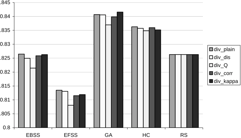
In Figure 1, the ensemble accuracy is shown for different search strategies including simple random subspacing (RS), and for the five pairwise measures of diversity used within the fitness function (1). The best integration method was selected for each data set, and the results were averaged over all the 21 data sets.

Figure 1. Average test set accuracy for different search strategies and guiding diversities

From Figure 1, one can see that the GA was the best on average, and the HC strategy was the second best. These two strategies are based on random subsampling (RS), which shows very good results on these data sets in itself. RS was better than EFSS for all the diversities, and better or equal than EBSS. Surprisingly, after it was the best for the Acute Abdominal Pain data sets in [38], EFSS was significantly worse than all the other strategies for this collection of data sets. This is more in line with the results of Aha and Bankert [1], which show that, for simple feature selection, backward sequential selection is often better than forward sequential selection as forward selection is not able to include groups of correlated features that do not have high relevance as separate features, only as a group.

There is no significant difference in the use of the guiding diversities. The only two significant dependencies found are: (1) div_Q is significantly worse than the other diversities for EBSS, EFSS, and the GA; and (2) div_kappa is better than the other diversities for the GA. The first dependency is expected and goes in line with the results presented in Tables 1 and 2. The second dependency is

0.8 0.805 0.81 0.815 0.82 0.825 0.83 0.835 0.84 0.845

EBSS EFSS GA HC RS

unexpected and can be explained, probably, by the peculiarities of the genetic search. HC is not that sensitive to the choice of the guiding diversity, as it starts with the already accurate ensemble (RS), and the search is not global as in the GA.

0.836 0.837 0.838 0.839 0.84 0.841 0.842

div_plain div_dis div_Q div_corr div_kappa

1 gen

5 gens

10 gens

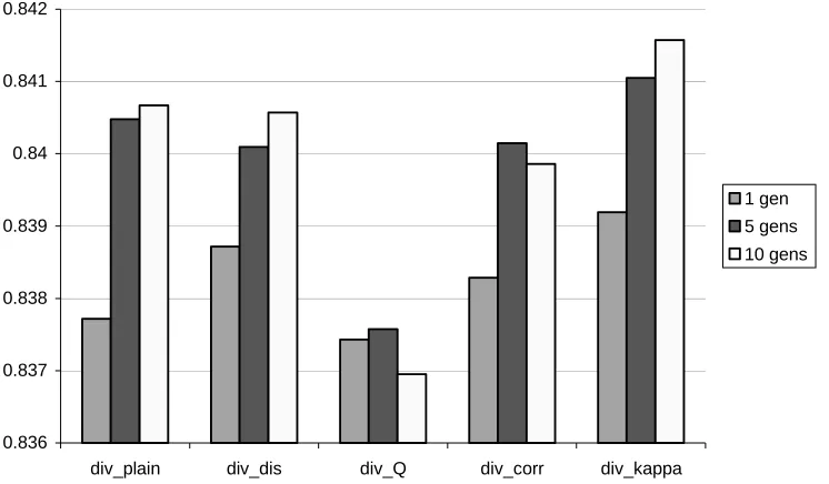
Figure 2. Average test set accuracy for different numbers of generations in the GA search strategy with different guiding diversities

In Figure 2, the average ensemble accuracy is shown for the GA strategy with the five guiding diversities after 1, 5, and 10 generations. From this figure, one can see that ensembles for all the diversities show improvement as the search progresses for the number of generations from 1 to 5. Then, ensembles built with div_Q and div_corr begin to degenerate, while the other ensembles still improve the average accuracy, though this improvement starts to tail off. This corresponds to the results presented in Tables 1 and 2, where these two measures of diversity have shown the worst average correlation with the difference between the ensemble accuracy and the average base classifier accuracy for DVS. As was also shown in the previous figure, the best diversity for the GA is div_kappa.

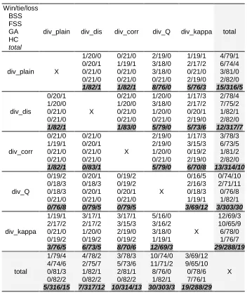
Each cell of Table 4 compares the diversity metric corresponding to the line against the metric corresponding to the column, and contains win/tie/loss information over the 21 data sets for the four search strategies correspondingly (EBSS, EFSS, GA, and HC), and in total (these numbers are given in gray, bold and italic). For each line and for each column we have also calculated the total numbers, which compare corresponding diversity against all the others, summing up corresponding cells.

Table 4. Student’ s t-test results comparing guiding diversities for different search strategies on 70 cross-validation runs Win/tie/loss BSS FSS GA HC total

div_plain div_dis div_corr div_Q div_kappa total

div_plain X

1/20/0 0/20/1 0/21/0 0/21/0 1/82/1 0/21/0 1/19/1 0/21/0 0/21/0 1/82/1 2/19/0 3/18/0 3/18/0 0/21/0 8/76/0 1/19/1 2/17/2 0/21/0 2/19/0 5/76/3 4/79/1 6/74/4 3/81/0 2/82/0 15/316/5 div_dis 0/20/1 1/20/0 0/21/0 0/21/0 1/82/1 X 0/21/0 1/20/0 0/21/0 0/21/0 1/83/0 1/20/0 3/18/0 1/20/0 0/21/0 5/79/0 1/17/3 2/17/2 0/20/1 2/19/0 5/73/6 2/78/4 7/75/2 1/82/1 2/82/0 12/317/7 div_corr 0/21/0 1/19/1 0/21/0 0/21/0 1/82/1 0/21/0 0/20/1 0/21/0 0/21/0 0/83/1 X 2/19/0 2/19/0 1/20/0 0/21/0 5/79/0 1/17/3 3/15/3 0/19/2 2/19/0 6/70/8 3/78/3 6/73/5 1/81/2 2/82/0 13/314/10 div_Q 0/19/2 0/18/3 0/18/3 0/21/0 0/76/8 0/20/1 0/18/3 0/20/1 0/21/0 0/79/5 0/19/2 0/19/2 0/20/1 0/21/0 0/79/5 X 0/16/5 2/16/3 0/18/3 1/19/1 3/69/12 0/74/10 2/71/11 0/76/8 1/82/1 3/303/30 div_kappa 1/19/1 2/17/2 0/21/0 0/19/2 3/76/5 3/17/1 2/17/2 1/20/0 0/19/2 6/73/5 3/17/1 3/15/3 2/19/0 0/19/2 8/70/6 5/16/0 3/16/2 3/18/0 1/19/1 12/69/3 X 12/69/3 10/65/9 6/78/0 1/76/7 29/288/19 total 1/79/4 4/74/6 0/81/3 0/82/2 5/316/15 4/78/2 2/75/7 1/82/1 0/82/2 7/317/12 3/78/3 5/73/6 2/81/1 0/82/2 10/314/13 10/74/0 11/71/2 8/76/0 1/82/1 30/303/3 3/69/12 9/65/10 0/78/6 7/76/1 19/288/29 X

the GA (6 wins and no losses) and it works well for EBSS (12 wins against 3 losses), however, it is very unstable for EFSS (10 wins and 9 losses). The other differences are insignificant.

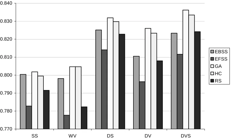
As the rest of the dependencies presented in this section do not depend on what guiding diversity is used, we consider them only for div_plain as the guiding diversity. In Figure 3, the average ensemble accuracies for the five integration methods (SS, WV, DS, DV, and DVS) are shown in combination with the four search strategies (EBSS, EFSS, GA, and HC) and RS.

0.770 0.780 0.790 0.800 0.810 0.820 0.830 0.840

SS WV DS DV DVS

EBSS EFSS GA HC RS

Figure 3. Average test set accuracy for different integration methods with different search strategies

From Figure 3, one can see that the dynamic methods always work better on average than the static methods, and DVS is the best dynamic method, that supports the conclusions presented in [38, 39]. DVS for the GA shows the best accuracy, and DVS with HC is the second best. For each of the dynamic methods, the ranking of the search strategies is the same: GA, HC, EBSS, RS, and EFSS.

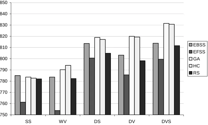
5.4 Average test set accuracy for different search strategies and integration methods on data sets with different numbers of features

0.750 0.760 0.770 0.780 0.790 0.800 0.810 0.820 0.830 0.840 0.850

SS WV DS DV DVS

EBSS EFSS GA

HC RS

Figure 4. Average test set accuracy for different integration methods with different search strategies for data sets with the number of features less than 9 (10 data sets)

0.750 0.760 0.770 0.780 0.790 0.800 0.810 0.820 0.830 0.840 0.850

SS WV DS DV DVS

EBSS EFSS GA

HC RS

Figure 5. Average test set accuracy for different integration methods with different search strategies for data sets with the number of features more than or equal to 9 (11 data sets)

5.5 Integration methods and the GA search strategy

0.780 0.790 0.800 0.810 0.820 0.830 0.840

SS WV DS DV DVS

1 gen 5 gens

10 gens

Figure 6. Average test set accuracy for different integration methods with the GA search strategy for different numbers of generations

5.6 Overfitting in the search strategies and integration methods

0.740 0.760 0.780 0.800 0.820 0.840 0.860 0.880 0.900

EBSS EFSS GA HC RS

Validation Test

Figure 7. Overfitting for different search strategies with the DVS integration method (test set and validation set accuracies)

0.740 0.760 0.780 0.800 0.820 0.840 0.860 0.880 0.900

SS WV DS DV DVS

Validation

Test

Figure 8. Overfitting for different integration methods averaged over the search strategies (test set and validation set accuracies)

5.7 Pre-selected alpha for integration methods and search strategies

0.0 0.5 1.0 1.5 2.0 2.5 3.0 3.5

SS WV DS DV DVS

EBSS EFSS

GA HC

Figure 9. Average pre-selected alpha values for different integration methods and search strategies

5.8 Average numbers of features selected for different search strategies and integration methods

0.0 0.1 0.2 0.3 0.4 0.5 0.6 0.7

EBSS EFSS GA HC RS

SS WV DS DV DVS

Figure 10. Average relative numbers of features in the base classifiers for different search strategies and integration methods

5.9 Pre-selected neighborhood for dynamic integration

0 5 10 15 20 25 30 35 40

DS DV DVS

EBSS EFSS GA HC RS

Figure 11. Average numbers of nearest neighbors pre-selected for the dynamic integration methods

Conclusions

In our paper, we have considered seven diversity metrics, five of which are pairwise and can be used as a component of the fitness function to guide the process of ensemble training in ensemble feature selection (the plain disagreement, div_plain; the fail/non-fail disagreement, div_dis; the Q statistic,

div_Q; the correlation coefficient, div_corr; and the kappa statistic, div_kappa), and two non-pairwise

(entropy, div_ent; and ambiguity, div_amb). All the seven measures can be used to measure the total ensemble diversity as a characteristic of ensemble goodness.

We consider four search strategies for ensemble feature selection: Hill Climbing (HC), a Genetic Algorithm for ensemble feature selection (GA), Ensemble Forward Sequential Selection (EFSS), and Ensemble Backward Sequential Selection (EBSS). In our implementation, all these search strategies employ the same fitness function, which is proportional to accuracy and diversity of the corresponding base classifier. Diversity in this context can be one of the five pairwise diversities considered. To integrate the base classifiers generated with the search strategies, we use five integration methods: Static Selection (SS), Weighted Voting (WV), Dynamic Selection (DS), Dynamic Voting (DV), and Dynamic Voting with Selection (DVS).

difference between the ensemble accuracy and the average base classifier accuracy. The correlations did not depend on the search strategy used, and depend significantly on the data set. The best correlations averaged over the 21 data sets were shown by div_plain, div_dis, div_ent, and div_amb.

Div_Q and div_corr behaved in a similar way, supported by the similarity of their formulae.

Surprisingly, div_Q had the worst average correlation. All the correlations besides div_Q and div_corr changed with the change of the integration method, showing the different use of diversity by the integration methods. The correlation coeffitients for Div_amb were almost the same as for div_plain.

Then, we have compared ensemble accuracies of the four search strategies for the five pairwise diversity metrics, and for the five integration methods being used. For all the diversities, the GA was the best strategy on average, and HC was the second best. The power of these strategies can be explained by the fact that they are based on random subsampling. Surprisingly, EFSS was significantly worse than the other strategies for this collection of data sets. There was no significant difference found in the use of the guiding diversities, besides the findings that div_Q was significantly worse on average than the other diversities for EBSS, EFSS, and the GA; and div_kappa was better than the other diversities for the GA. HC was not sensitive to the choice of the guiding diversity. The results of the Student’ s t-test for significance supported these findings. The dynamic integration methods DS, DV, and DVS always worked better on average than the static methods SS and WV, and DVS was the best dynamic method on average. The GA and DVS was the best combination of a search strategy and integration method.

To analyse overfitting in these ensembles, we have measured all the ensemble accuracies on both the validation and test sets. Among the search strategies, GA and EFSS had the biggest overfitting on average. For the integration methods, it was discovered that the static integration methods show more overfitting than their dynamic counterparts.

The experimental results presented change very much with the data set, and more data sets are needed to check and to analyse the reported findings. More experiments are needed to check how the behaviour of the diversity metrics depends on the data set characteristics, and what is the best metric for a particular data set. This is an interesting topic for further research.

References

[1] D.W. Aha, R.L. Bankert, A comparative evaluation of sequential feature selection algorithms, in: D. Fisher, H. Lenz (Eds.), Proc. 5th Int. Workshop on Artificial Intelligence and Statistics, 1995, pp. 1-7.

[2] E. Bauer, R. Kohavi, An empirical comparison of voting classification algorithms: bagging, boosting, and variants, Machine Learning, 36 (1,2) (1999) 105-139.

[3] C.L. Blake, E. Keogh, C.J. Merz, UCI repository of machine learning databases [http:// www.ics.uci.edu/ ~mlearn/ MLRepository.html], Dept. of Information and Computer Science, University of California, Irvine, CA, 1999.

[4] C. Brodley, T. Lane, Creating and exploiting coverage and diversity, in: Proc. AAAI-96 Workshop on Integrating Multiple Learned Models, Portland, OR, 1996, pp. 8-14.

[5] P. Chan, An extensible meta-learning approach for scalable and accurate inductive learning. Dept. of Computer Science, Columbia University, New York, NY, PhD Thesis, 1996 (Technical Report CUCS-044-96).

[6] P. Chan, S. Stolfo, On the accuracy of meta-learning for scalable data mining. Intelligent Information Systems 8 (1997) 5-28.

[7] L.P. Cordella, P. Foggia, C. Sansone, F. Tortorella, M. Vento, Reliability parameters to improve combination strategies in multi-expert systems, Pattern Analysis and Applications 2(3) (1999) 205-214.

[8] P. Cunningham, J. Carney, Diversity versus quality in classification ensembles based on feature selection, in: R.L. deMántaras, E. Plaza (eds.), Proc. ECML 2000 11th European Conf. On Machine Learning, Barcelona, Spain, LNCS 1810, Springer, 2000, pp. 109-116.

[9] T.G. Dietterich, An experimental comparison of three methods for constructing ensembles of decision trees: bagging, boosting, and randomization, Machine Learning 40 (2) (2000) 139-157. [10] T.G. Dietterich, Machine learning research: four current directions, AI Magazine 18(4) (1997)

97-136.

[11] T.G. Dietterich, G. Bakiri, Solving multiclass learning problems via error-correcting output codes, Journal of Artificial Intelligence Research 2 (1995) 263-286.

[12] P. Domingos, M. Pazzani, On the optimality of the simple Bayesian classifier under zero-one loss, Machine Learning, 29 (2,3) (1997) 103-130.

[14] G. Giacinto, F. Roli, Methods for dynamic classifier selection, in: Proc. ICIAP '99, 10th Int. Conf. on Image Analysis and Processing, IEEE CS Press, 1999, pp. 659-664.

[15] L. Hansen, P. Salamon, Neural network ensembles, IEEE Transactions on Pattern Analysis and Machine Intelligence, 12 (1990) 993-1001.

[16] D. Heath, S. Kasif, S. Salzberg, Committees of decision trees. In: B. Gorayska, J. Mey (eds.), Cognitive Technology: in Search of a Humane Interface, Elsevier Science, 1996, pp. 305-317. [17] T.K. Ho, The random subspace method for constructing decision forests, IEEE Transactions on

Pattern Analysis and Machine Intelligence, 20 (8) (1998) 832-844.

[18] R. Kohavi, Wrappers for performance enhancement and oblivious decision graphs, Dept. of Computer Science, Stanford University, Stanford, USA, PhD Thesis, 1995.

[19] R. Kohavi, D. Sommerfield, J. Dougherty, Data mining using MLC++: a machine learning library in C++, Tools with Artificial Intelligence, IEEE CS Press (1996) 234-245.

[20] M. Koppel, S. Engelson, Integrating multiple classifiers by finding their areas of expertise, in: AAAI-96 Workshop On Integrating Multiple Learning Models for Improving and Scaling Machine Learning Algorithms, Portland, OR, 1996, pp. 53-58.

[21] A. Krogh, J. Vedelsby, Neural network ensembles, cross validation, and active learning, In: D. Touretzky, T. Leen (Eds.), Advances in Neural Information Processing Systems, Vol. 7, Cambridge, MA, MIT Press, 1995, pp. 231-238.

[22] L.I. Kuncheva, C.J. Whitaker, Measures of diversity in classifier ensembles and their relationship with the ensemble accuracy, Machine Learning 51 (2) (2003) 181-207.

[23] D.D. Margineantu, T.G. Dietterich, Pruning adaptive boosting, in: Proc. 14th Int. Conf. on Machine Learning, Morgan Kaufmann, 1997, pp. 211-218.

[24] C.J. Merz, Classification and regression by combining models, Dept. of Information and Computer Science, University of California, Irvine, USA, PhD Thesis, 1998.

[25] C.J. Merz, Dynamical selection of learning algorithms, in: D. Fisher, H.-J. Lenz (eds.) Learning from Data, Artificial Intelligence and Statistics, Springer, 1996.

[26] C.J. Merz, Using correspondence analysis to combine classifiers, Machine Learning 36 (1-2) (1999) 33-58.

[27] D. Opitz, Feature selection for ensembles, in: Proc. 16th National Conf. on Artificial Intelligence, AAAI Press, 1999, pp. 379-384.