Three phase power system harmonic penetration

THREE PHASE POWER SYSTEM

HARMONIC PENETRATION

A thesis

presented for the degree of

Doctor.of Philosophy in Electrical Engineering in the

University of Canterbury, Christchurch, New Zealand

by

T.J. Densem B.E. (Hons)

iK

1010

.D113

1~g3 Harmony would lose its attractiveness if it did not have a background of discord.

Li st of Fi gures List of Tables

List of Principal Symbols Abstract

Acknowledgements

CHAPTER 1 INTRODUCTION

;

TABLE OF CONTENTS

CHAPTER 2 REVIEW OF POWER SYSTEM HARMONICS 2.1 Basic Concepts

2.2 Harmonic Power Flows

2.3 Harmonic Effects on Power System Plant . 2.4 Harmonic Modelling

v x xi xiii \ xv 1 3 3 4 6 7

2.4.1 Introduction 7

CHAPTER 3

2.4.2' Balanced Harmonic Penetration 7

2.4.3 System Impedances for Filter Design 8

2.4.4 Unbalanced Convertor Operation 10

'2.5 Measurement of Harmonics

2.6 Measurement and Modelling Correlation

ALGORITHM DEVELOPMENT

3.1 Introduction

3.2 Requirements for Harmonic Modelling 3.3 Single Phase Modelling

3.4 Thr~e Phase Algorithms

3.5 Three Phase Harmonic Penetration

3.6 Formation of the Nodal Admittance Matrices 3.6.1 3.6.2 3.6.3 3.6.4 3.6.5 3.6.6 3.6.7 Introduction

Network Subdivision Linear Transformation Shunt and Series Elements Coupled Shunt Elements

Combined Series and Shunt Connected Elements

Forming the System Admittance Matrix

3.7 Conclusions

CHAPTER 4

CHAPTER 5

CHAPTER 6

CHAPTER 7

MODELLING OF NEAR BALANCED COMPONENTS 4.1 Introduction

4.2 Shunt Capacitors 4.3 Filters

4.4 Synchronous Generators 4.5 Load Modelling

4.6 Transformer Modelling 4.7 Conclusions

TRANSMISSION LINE MODELLING

39 39 39 40 40 41 45 48 49

5.1 Introduction 49

5.2 Single Phase Line Model 51

5.3 Multiconductor Transmission Line Modelling 56

5.4 Skin Effect Modelling 59

5.5 App 1 i ca ti ons of the Computer Model 65 5.5.1 Harmonics Generated Along Transmission

Lines 65

5.5.2 Zero Sequence Harmonics in Transmission

Lines Connected to Static Convertors 69 5.6 Phase Differences

5.7 Mutual Coupling of Double Circuit Lines 5.8 Conclusions

REDUCED TEST SYSTEM

75 78 81 82

6.1 Introduction 82

6.2 Generator, Transformer and Load Impedances 83 6.3 Connection of Components to Transmission Lines 84

6.4 Six Line System 87

6.5 Eight Line System 89

6.6 Voltage Sensitivity to Line Parameter Variation 92 6.7 Three Phase Impedances of the Reduced System 94

6.8 Harmonic Unbalance Factor 94

6.9 Conclusions 97

THREE PHASE HARMONIC PENETRATION 7.1 Introduction

7.2 Test System 7.3 Model Selection

CHAPTER 8

CHAPTER 9

iii

7.4 Voltage Sensitivity to Individual Component

Impedances 106

7.4.1 Introduction 106

7.4.2 ·7.4.3 7.4.4

Transformer Impedance Variation Generator Impedance Variation Load Level Variation

106 109 112

7.4.5 Line Parameter Variation 117

7.5 Comparison of Measured and Simulated Voltages 120

7.6 Impedance Imbalance. 122

7.7 Circuit Coupling 125

7.8 Single Phase Modelling 128

7 .. 9 Network Assumptions 131

7.9.1 Temperatur~ Variation 131

7~9.2 Skin Effect 131

7.9.3 Earth Resistivity Variation 7.10 Unbalanced Harmonic Current Injections 7.11 System Configuration Change

7.12 Conclusions

RIPPLE CONTROL SPILLOVER

131 136 138 139

141

8.1 Introduetion 141

8.2 Program Comparison 144

8.3 Test System 145

8.4 Voltage Sensitivity to Individual Component

Impedances 146

8.4.1 Transformer Impedance Variation 146 8.4.2

8.4.3

Generator Impedance Variation Load Level Variation

148 150

8.4.4 Line Parameter Variation 152

8.5 Model Variations 154

8.6 Filters and Shunt Capacitors 157

8.7 Single Phase Modelling 159

8.8 Spillover Voltages for Different Frequencies l62

8.9 Conclusions 164

CONCLUS IONS 166

APPENDIX 1

APPENDIX 2

APPENDIX 3

APPENDIX 4

Data for the Reduced Test System 176

Data for the New Zealand South Island System Below Bromley 179

Data for the New Zealand South Island System in 1985 184

Published Paper "Zero Sequence Harmonic Current Generation 197 in Transmission Lines Connected to Large Convertor Plant", IEEE Trans. PAS-102, No.7, pp 2357-2363.

Paper Accepted for Publ i cati on. "Three Phase Transmi ss ion Systems Modelling for Harmonic Penetration Studies " ,

Figure 2.1 2.2 2.3 2.4 2.5 2.6 2.7 2.8 2.9 2.10 3.1 3.2 3.3 3.4 3.5 3.6 3.7 3.8 3.9 3.10 3.11 3.12 3.13

LIST OF FIGURES

Schematic of Power Flow in the AC System

Schematic of Fundamentai Frequency PoweY' Flow

Schematic of Harmonic Power Flow

Balanced Current Injection Into a Balanced AC System

Unbalanced Current Injection into an Unbalanced AC System

Filters Connected to a Convertor Busbar

Three Phase Convertor with Approximate System Impedances

Convertors Attached to Different Busbars of the Unbalanced AC System

Schematic of Harmonic Measurement System

Harmonic Impedance versus Frequency of the Bonneville Power Administration System from Celilo HVDC Substation

Structure Diagram of Sing~ Phase Modelling

Structure Diagram of Three Phase ~odelling

Data Flow Diagram

Structure Diagram of Three Phase Harmonic Penetration Program

Solution of h Linear Simultaneous Equations

Three Convertors Attached to Different Busbars on the AC System

Reduced Three Convertor System

Two Port Network Transmission Parameters

Representation of a Shunt Element

Representation of a Series Element

Two Winding Three Phase Transformer as Two Coupled Compound Admittances

Series and Shunt Connected Element

Three Phase Combined Series and Shunt Connected Elements

Figure 4.1 4.2 4.3 4.4 5.1 5.2 5.3 5.4 5.5 5.6 5.7 5.8 5.9 5.10 5.11 5.12 5.13 5.14 5.15 5.16 5.17 5.18

Shunt Capacitor Representation

HVDC Shunt Filter Types

Schematic Representation of Supply Authority Distribution Network

Equivalent Circuit for Symmetrical Star-gldelta Transformer (unity tap ratio)

Nominal PI Transmission Line Model

The Equivalent PI Model of a Long Transmission Line

Equivalent PI Impedances

Impedance Versus Frequency for the Equivalent PI Model

Impedance Versus Frequency for the Open Ci rcu; ted Islington to Kikiwa Transmission Line

Comparison of the Equivalent and Nominal PI Transmission Line Models

Conductor Information for the Islington to Kikiwa Line

Structure Diagram for the Equivalent PI Model

Skin Effect Resistance Ratios for Different Models

ACSR Conductor Hollow Tube Representation

The Effect of Skin Effect Modelling

Positive Sequence Voltage Versus Frequency along the Open Ended Islington to Kikiwa Line

Sequence Currents along the Open Ended Line for a 1 pu Positive Sequence Current Injection

Sequence currents Along the Short Circuited Line for a 1 pu Posi~ive Sequence Current Injection

Zero Sequence Current Versus Frequency for a 1 pu Zero Sequence Current Injection

Sequence Currents for a 1 pu Positive Sequence Current Injected into a Transformer and Line

Sequence Currents for a 1 pu Positive Sequence Current in the Presence .of a Convertor Transformer and

Fi lters

Sequence Currents for a 1 pu Positive Sequence Current Injection with a Parallel Resonance Between the Line and Fi 1 ters

vii

Figure

5.19 Sequence Currents for a 1 pu Positive Sequence Current Injection with One Phase of the Fi lter Ban k Open

Circuited ' 7 4

5.20 Three Phase Resonant Frequencies of the Islington to

Kikiwa Line with a Balanced 1 pu Current Injection 76 5.21 Three Phase Resonant Frequencies for the Transposed Line 77

5~22 Conductor Information for the Double Circuit Line 78

5.23 Sequence Impedance Magnitude Versus Frequency for the

Double Circuit Coupled Line 79

5.24 Sequence Impedance Magnitude versus Frequency for Two

Single Circuit Lines 79

6.1 Polar Plot of the Generator, Transformer and Load

Impedances at Roxburgh 83

6.2 Positive Sequence Voltage Magnitude at Invercargill versus Frequency for Differing Terminations of the Roxburgh to

Invercargill Lines 85

6.3 Positi ve Sequence Voltage Phase Angles at Invercargi 11 versus Frequency for Different Terminations of the Roxburgh

to Invercargill Lines 85

6.4 Polar Plot of the Impedance of the Open Circuited

Invercargill to Roxburgh Lines with 50 Hz Intervals Marked 86

6.5 Six Line System Including Load and Generation 87

6.6 Positive Sequence Voltage Magnitude at Tiwai Versus

Frequency for Di fferent Termi nati ons 88

6.7 Reduced System Including Load and Generation 89

6.8 Positi ve Sequence Voltage IViagnitude versus Frequency

for Different Terminations 90

6.9 Positive Sequence Phase Angles at Tiwai versus

Frequency for Different Terminations 90

6.10 Positive Sequence Impedances of the Reduced System from

Tiwai wi th Harmoni c Intervals Indi cated 91

6.11 Positive Sequence Voltage Magnitude versus Frequency at

all Reduced System Busbars 91

6.12 Positive Sequence Voltage Magnitude versus Frequency for

Line Length Variation 93

Figure

7.1 New Zealand South Island Transmission System Below Bromley 99

7.2 Summary of Component Models 104

7.3 Measured and Simulated Yellow Phase Characteristic Harmonic Impedances for the South Island Transmission

System from Tiwai 220 kV Busbar 105

7.4 7.5 7.6 7.7 7.8 7.9 7.10 7.11 7.12

Percentage Voltage for Transformer Impedance Variation Percentage Voltage for Generator Impedance Variation Percentage Voltage for Load Level Variation

Percentage Voltage on No Load

Percentage Voltage for Line Length Variation Phase Impedances for the South Island System

Sequence Voltages at Selected Busbars for Positive .Sequence Current Injection at Tiwai Normalized to 1 pu

Percentage Voltage for Circuit Coupling

Percentage Voltage for Single Phase Modelling

107 110 113 115 118 122 124 126 129 7.13 Percentage Voltage for Temperature Variation and Skin Effect

Modelling 132

7.14 Percentage Voltage for Resistivity Variation 134

7.15 7.16 8.1 8.2 8.3 8.4 8.5 8.6 8.7 8.8 8.9

Sequence Voltages at Selected Busbars for Unbalanced Current Injection at Tiwai

Positive Sequence Voltages at Selected Busbars with both Lines from Tiwai to Manapouri Open Circuited. Current Injection at Tiwai Normalized to 1 pu

Schematic of Ripple Control Spillover

Ripple Contro; Spillover Areas for Central Canterbury Electric Power Board

Central Canterbury Electric Power Board Ripple Control

Injection at Hornby .

Percentage Voltage for Transformer Impedance Variation Percentage Voltage for Generator Impedance Variation Percentage Voltage for Load Level Variation

Percentage Voltage for Line Length Variation Percentage Voltage for Model Variation

Percentage Voltage due to Filters and Shunt Capacitors

Figure

8.10

8.11

A1.1 A2.1

A3.1

Percentage Voltage Using Single Phase Modelling . Percentage Voltage Using Three Different Harmonic

Penetration Programs Transformer Connection

S"ingle Line Diagram for the South Island System below Bromley

Single Line Diagram of the New Zealand South Island System in 1985

Page

160

161 176 183

LIST OF TABLES

5.1 Harmonic Voltage Measurements during Back-to-Back Testing of the New Zealand DC Link while Commissioning

in 1966 . 50

5.2 Tube Ratios for Commonly Used Conductors 63

7.1 Comparison of Voltages for the System Below Bromley

and the Whole South Island Network 100

7.2 Current Injections at Tiwai for 7 Rectiformer Operation 101 7.3 Measured and Simulated Values of Harmonic Impedances at

Tiwai with Different Generato~ Load and Transformer Models 103 7.4 Comparison of Measured and Simulated Harmonic Voltages 121 7.5 23rd Harmonic Impedance Magnitudes at Tiwai for Single

Ci rcui t Outage 138

8.1 Features of the Three Harmonic Programs Available in

New Zealand 144

8.2 Spillover Voltage Levels For Central Canterbury Electric

Power Board at 510 Hz and 317 Hz 163

A1.1 Reduced System Busbars and Loading 177

A1.2 Reduced System Generation 177

A1.3 Reduced System Transformers 177

A1.4 Line Data for the Reduced System 178

A2.1 Busbarsand Loading for the South Island System Below

Bromley 180

A2.2 Generation for the South Island System Below Bromley 181 A2.3 Transformers for the South Island System Below Bromley 181 A2.4 Transmission Line Data for the New Zealand South Island

System Below Bromley 182

A3.1 Busbars and Loading for the South Island System in 1985 185 A3.2 Transformers for the South Island System in 1985 188 A3.3 Generation for the South Island System in 1985 190 A3.4 Transmission Line Data for the New Zealand South Island

a abc ABCD AC AC/DC C

[c]

[M]

pas

[v]

LIST OF PRINCIPAL SYMBOLS

transformer tap ratio phase components

transmission line parameters alternating current

alternating to direct current conversion capacitance

connection matrix direct current equivalent PI model frequency

generator

geometric mean radius . harmon; corder

high voltage direct current current at harmonic h

inductance

matrix of normalized eigenvectors nominal PI model

primary

point of common coupling real power

point of injection point of supply primitive

per unit

reactive power radius

resistance

red, yellow and blue phases secondary

thickness

voltage at harmonic h length

shunt admittance matrix

[zJ

Zl

+ - 0

series impedance matrix

series impedance of a transmission line per unit length filter impedance at harmonic h

AC system impedance at harmonic h characteristic impedance

sequence components attenuation constant phase constant

xiii

ABSTRACT

Three phase harmonic penetration software is developed and tested using measured results from the New Zealand power system.

The unbalanced nature of the impedances. currents and voltages usually present in a power system is illustrated. The versatility of the algorithm to provide accurate information for studies of convertor interaction and single phase traction supplies is clearly indicated.

Practical problems encountered in harmonic modelling are discussed, particularly the adequacy of available component data and the validity of models using this data.

Harmonic spillover interference- to load management equipment

operating above fundamental power frequencies is of practical significance. and the levels of such interference fot a proposed frequency change are investigated:

A commitment to three phase modelling must be justified, and

ACKNOWLEDGEMENTS

I wish to express my sincere thanks to my supervisors, Professor J. Arrillaga, Dr P. Bodger and Dr B. Harker for their

advice, assistance and loyalty throughout the course of this research.

Special recognition is due to my employer, New Zealand Electricity. The wholehearted technical and financial support of this research is

deeply appreciated.

The intial financial help of the University Grants Committee is gratefully acknowledged as is the technical assistance given by Chris Currie, John Baird, Hermann Dommel and Neville Ross. Their experience and helpful advice has been invaluable.

Thanks are due to my postgraduate colleagues for their useful comments and words of encouragement. The computer results in this thesis would not have been possible without the tireless efforts of Bill Kennedy and the graphics software written by Steve Gellen.

Christ"ine McEntee1s typing of this thesis has been excellent.

CHAPTER 1

INTRODUCTION.

Problems associated with the propagation of harmonic currents in electric power systems are extensive, affecting both the economics of operation and security of supply. The cost of interference with load management equipment and telephone circuits is large, and the solutions expensive. Also, the failure of power system components and the

maloperation of equipment as a result of high levels of harmonic voltages and currents causes less secure system operating conditions. These wide repercussions, coupled with increasing levels of harmonics, have prompted interest in analysis of the penetration of harmonics in power systems.

An understanding of harmonic penetration requires the coordinated development of both measurement and digital computer simulation techniques. This thesis discusses the simulation aspect, combining the techniques

used in fundamental frequency three phase power flow and single phase harmonic modellin~ to develop three phase harmonic penetration software. The use of unbalanced analysis in three phase systems leads to more accurate simulation of the propagation of harmonics.

In Chapter 2 some fundamental concepts of harmonic analysis in power systems are discussed and the limitations of present modelling techniques are illustrated using comparisons with measured data. Often measurement is not practical at harmonic frequencies,and simulation is presented as a complementary tool to measurement techniques in this situation.

Chapter 3 discusses the development of harmonic modelling leading to the present work in three phases. Requirements for harmonic software are stated, and the need for a different approach to that used in single phase modelling is indicated. The purpose of the individual programs is explained and the development of the penetration program, HARMAC, is described. Admittance matrix techniques are utilized and the inclusion of sjstem elements into these matrices using phase components is detailed.

Chapter 5 details the modelling of three phase transmission lines including skin effect. The ability of the three phase model to match known unbalanced conditions is confirmed and the effect on system harmonic levels of convertor transformer connection is investigated.

In Chapter 6 a small test system is progressively developed to assist in the understanding of harmonic penetration, without the

complications of a large interconnected grid. The damping and resonant effects of the transformers, generators and loads are discussed. The connection of unbalanced harmonic loads is simulated showing the ability of three phase techniques to accurately model such situations.

Chapter 7 utilises test results to confirm modelling techniques on a large power system. The sensitivity of system voltages to

variations in individual component impedances is used to determine the adequacy of present data. Single phase and three phase analysis

techniques are also compared and a number of different cases are tested to i 11 ustrate the versatility of the software.

Chapter 8 studies the problem of ripple control spillover, where load management signals from a distribution authority penetrate, via the transmission system, to other distribution authorities. If the ripple relays are sensitive to these signals then unscheduled load switching can occur. The differences between single phase and three phase modelling techniques are illustrated on the complete system of the South Island of New Zealand.

CHAPTER 2

REVIEW OF POWER SYSTEM HARMONICS

2.1 BASIC CONCEPTS

A number of terms are commonly referred to in the field of power system harmonics. A harmonic is defined as a sinusoid whose frequency is an integral multiple of the actual system frequency. The order of a harmonic is the ratio of the harmonic frequency to the fundamental frequency. Harmonic analysis is described as the process of measuring or calculating the. magnitude and phase of the harmonic components

contained in a waveform. The full set of harmonics present forms a Fourier series which, when summated, replicates the original waveform.

When a non-sinusoidal waveform is viewed on an oscilloscope its shape is observed in the time domain. That is, for any given instant in time, the amplitude of the waveform ;s displayed. Time is normally drawn on the horizontal axis with increasing time to the right. This waveform can also be described in the frequency domain. If the basic repetition frequency of a square wave was say 50 Hz, and it was applied to a hi-fi amplifier, then the ear would hear the resultant sound as a mixture of many frequencies. That is, it would sound like a full musical chord. The waveform may therefore be described by its time domain data or its frequency domain data. The transfer from the time domain to the frequency domain is accomplished by a Fourier transformation.

The function of a power system is to provide consumers with a

purely sinusoidal voltage supply of constant amplitude and frequency. The presence of harmonics causes the character of the supply to deviate from this ideal by introducing distortion into the wave shape.

Power system harmonics are not new phenomena. As a form of power system pollution harmonics have been present since the inception of alternating current systems, generated by components such as transformers. The linearity of transformer magnetic circuits results in a

The major contribution to system harmonic content comes from the various non-linear loads connected to the transmission networ~ of which the most important are the various forms of static power convertor. Harmonics are introduced into the power system by these devices due to the non-linear frequency relationship between voltage and current. The proliferation of non-linear HVDC plant and domestic appliances (Blommaent et al 1977, Carroll et al 1977~ Evers 1980 and Orr et al 1982) is on the increase, and will lead to increased harmonic levels.

The alternating current waveform associated with an HVDC convertor may be considered to be the smooth direct current distributed between the three phases of the AC system in the form of rectangular blocks. In turn, this rectangular wave shape can be considered as being composed of a

fundamental sinusoid and harmonic components. Only the fundamental is of prime interest in the transfer of power between the AC and DC systems. The harmonics are generally an unwanted product of the conversion process.

The study of harmonic currents and voltages propagating in the AC power system, is termed harmonic penetration. This thesis is concerned with harmonic penetration in the transmission system,which includes

modelling from the harmonic sources through the transmission lines to the generators and load centers.

2.2 HARt40N I C POWER FLOWS

To analyse harmonic power flows, the system equivalent circuit as depicted in Figure 2.1 has been used by Tschappu (1981). The generator G constitutes a fundamental sinusoidal voltage source and it supplies a resistive load controlled with a static convertor via the system impedance

Zs.

Figure 2.2 illustrates the equivalent circuit diagram for the fundamental frequency. The generator supplies, via the point of common coupling (PCC), the fundamental power PgI, which flows to a large extent as Pl1~ to the. load and to a lesser extent, as Pel to the convertor. This portion is transform(;!d into harmonic power .. In addition to this,

Psh + Pgh

PSI

~

I - - { ! T - - - I

[>IL1---1

PR~

G

R

pee

FIGU 2.1: Schematic of Power Flow in the AC System

PSI

r---1

Rs

X

[>ILr----;

G

pee

GURE 2.2: Schemati c of Fundamental Freguen'cy Power Flow

Ih

I

r---;Rs

X

,~~

<llI7Z~

R,

Pgh

:

I

I

I I I

pee

In Figure 2~3 the equivalent circuit diagram for the harmonic power flow is depicted. Since the generator voltage is sinusoidal it can only supply fundamental power and it is included in this diagram as a harmonic impedance. The convertor appears in place of the generator as an impressed harmonic current source. A small portion of the fundamental power Pc1, transformed into harmonic power~ is fed as Psh and Pgh back to the resistance of the system ~nd the generator, and the large portion,

P~h, to the load. Since Rs and Rt are connected in series, the ratio of

P~h/(Psh + Pgh) can also be expressed as R~/(Rs + Rg). In practice, .

~/(Rs + Rg) is very large, and for this reason, the portion of harmonic power propagating in the AC system remains small even when the current is badly distorted.

The total losses in the system impedance are composed of the

fundamental power PsI, supplied from the generator, and the harmonic power of the convertor, Psh + Pgh. The harmonic loss in the system incurred on. the generator side of the point of common coupling, is debited to the supply authority. This loss in the system is larger by the ratio

(Psh + Pgh)/Ps1 than with linear loading.

2.3 HARMONIC EFFECTS ON POWER SYSTEM PLANT

Whether or not the harmonic power.is considered as useful or unwanted, is dependent upon the type of load. If the harmonic power serves to

produce heat in a heating load, then it constitutes useful energy. However, when converting electrical power into mechanical \'JOrk, e.g. when using an induction motor, the harmonic power gives rise to additional heating in the stator and rotor windings. The efficiency of the motor is thereby reduced. In this case, the harmonic content of the supplied power is considered to be detrimental.

Other effects on power system equipment of a distorted supply are also documented .. They include telephone interference where liries run

"in close proximity to power transmission. lines (Kl·ewe 1958), protection

maloperation '(IEEE Working Group 1981), metering inaccuracies (Baggott 1974), losses (Klingshirn and Jordan 1968), capacitor failure (Gates 1979), ripple control spillover (Ross 1972) and unstable operation of static

convertors (Yacamini and de Oliveira 1980a).

2.4 HARMONIC MODELLING

2.4.1 Introduction

There are a number of areas where harmonic modelling can be usefully employed. The major assumptions in each area, the limitations and the extent to which more investigations are required, will be

discussed.

2.4.2 Balanced Harmonic Penetration

Figure 2.4 illustrates two sets of balanced harmonic currents, I1h and I2_h, of order h. injected into any busbar of an AC system. A large power system is likely to have a number of such injections. The resultant system harmonic voltages are calculated by direct solution of the linear equation:

=

BALANCED AC

SYSTEM

FIGURE 2.4: Balanced Current Injection into a Balanced AC System

An assumption generally made is that the AC system is balanced

(2.1)

and can therefore be modelled by the positive sequence component impedances

(~1cGranaghan et al 1981 and Breuer et al 1982). The validity of this

assumption will be examined in Chapters 7 and 8.

The above algorithm models the steady state behaviour of a power system. Unfortunately the harmonic behaviour of a physical system

changes as loads, generators and line configuration alter. It is difficult "'lith a steady state model to obtain more than a few "snap shots" of a

continuously varying system.

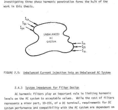
A power system is three phase and will have imbalance between phases due to transmission line conductor assymetry and load imbalance. By modelling these irrbalances, illustrated in Figure 2.5, more accurate simulations will be possible. In such a system the current injections, Ilh-I3h and I4h-I6h, can be unbalanced in magnitude and phase angle. In a similar manner to the balanced system the current injections for each frequency are presumed constant and known and the linear equation (2.1) is solved directly to obtain the three phase harmonic voltages.

Investigating three phase harmonic penetration forms the bulk of the work in this thesis.

UNBALANCED AC SYSTEM

"""",,1!III!IJ--11h

.... I--I

"..,-.-...

... --13h

FIGURE 2.5: Unbalanced Current Injection into an Unbalanced AC System

2.4.3 System Impedances for Filter Design

To achieve adequate performance levels requires information on

characteristic and non-characteristic harmonic generation of the convertor, harmonic impedances of the AC system, frequency swings, voltage swings and VAR requirements of the AC system (Lacoste et al 1979). This then allows the selection

of

In steady state operation, harmonic currents are determined by the convertor configuration and by the system parameters. Characteristic harmonics are produced by an ideal convertor (i.e. for a 12 pulse

convertor these will be 12k +/- 1, where k is a positive integer).

The Fourier series for the normalized current waveform of an ideal 12 pulse convertor is~

4 13 [ 1 1 ]

- n - cos (wt) -

IT

13

The harmonic magnitudes are equal to that of the fundamental current divided by the harmonic order (Arrillaga 1983),

(2.2)

All other harmonics are termed noncharacteristic and are produced by AC system voltage magnitude and phase imbalance, convertor transformer reactance di fferences and control fi r"j ng angl e assymmetry. The i njecti on of harmonic currents into the AC system results in harmonic voltages which are a function of the AC system harmonic impedance and harmonic

current flow throughout the AC network.

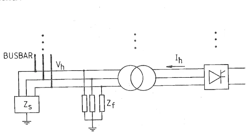
To mitigate the harmonic current flow into the network, filters are applied on the convertor bus as shown in the single line diagram of Figure 2.6. The model representation of Figure 2.6 shows the harmonic current flow into the combination of filter, Zf' in parallel with the system including generation and loads, Zs' which permits calculation of individual harmonic voltages, Vh .

CONVERTOR CURRENT SOURCE

PCC

Vh

FIGURE 2.6: F'lt _{1 ers onnected to a} C

_COnv9rtnr

_Busbar

Accurate system impedances are required because of the possibility of resonance between the filters and system impedances, and the need to meet both voltage and current specifications at the point of common coupling.

Initial design of filters for HVDC applications proved to be

unsatisfactory (Gunn 1966, Jarrett and Csuros 1966,and Huddart and Brewer 1966), a major reason being poor system impedance representation at harmonic

frequencies. Subsequent design concepts became conservative because of these experiences and the inability to match measured with simulated

system impedances (Laurent et al 1962 and Melvold 1972). After successful filter installations (Vithayathil 1973), attention has focussed on more appropriate filters by utilising better system impedance representation

(Breuer et al 1982 and Abramovich et al 1982). The attainment of more accurate system impedances will be investigated in Chapter 7.

2.4.4 Unbalanced Convertor Operation

Figure 2.7 illustrates an equivalent circuit suitable for the analysis of unbalanced.convertor operation. The convertor generates harmonic currents, ~, which propagate in the parallel system and filter impedances causing harmonic voltages to be present at the convertor terminal busbar. A number of convertors may be attached to the same busbar.

..

..

_..

_..

.,.

" <II

OIl

BUSBAR

_Ih

Vh

Early convertor investigations involving fundamental frequency imbalance were performed by Phadke and Harlow (1966). Considerable work on improved control strategies to solve harmonic instabilities was

initiated by Ainsworth (1967). Further investigations were performed on digital computers for harmonic voltage and firing angle imbalance by Reeve and Krishnayya (1968), Phadke and Harlow (1968) and Reeve et al (1969) .

The interaction of convertor current injections with system voltages, leading to a more accurate convertor representation, was undertaken by Reeve and Baron (1970). It was not until Yacamini and de Oliveira (1980a) that convertor interaction was generalised for any configuration at the injection bus. Transformer saturation was included in this study. The complete range of interactions including accurate DC system impedance modelling was discussed by Yacamini and de Oliveira (1980b) and Yacamini and Smith (1983).

The AC system in the above studies has been represented in an approximate form by either an impedance based on the short circuit ratio, a tee equivalent circuit Bowles (1970) or a balanced impedance locus, Reeve and Baron (1970). The first approach using the short circuit ratio is an unsatisfactory representation (Kauferle et al 1970), and only by using measured or simulated impedances calculated for the whole network can realistic studies be performed. Results using unbalanced AC systems have not been investigated. The provision of three phase impedance modelling will make this possible.

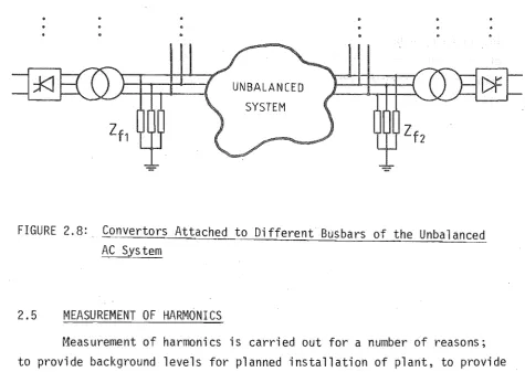
The situation with a single injection point into the AC system can be generalised to a number of injection points, each point being connected to a separate busbar. This is represented in Figure 2.8. The calculation of three phase system impedances will also enable such studies to be

performed.

A basic premise of the convertor analysis discussed, is that the fundamental frequency power flow is unaltered by the superposition of harmonic voltages at the point of harmonic injection into the AC system. Initial studies of the operating state of a convertor with

flow included have been performed by Xia and Heydt (1982). were however restricted to characteristic harmonics and no

results were presented.

12

UNBALANCED

SYSTEM

FIGURE 2.8: Convertors Attached to Different Busbars of the Unbalanced AC System

2.5 MEASUREMENT OF HARMONICS

Measurement of harmonics is carried out for a number of reasons; to provide background levels for planned installation of plant, to provide impedance data for filter design, to enforce harmonic limits, to determine the propagation of audio frequency control signals or to determine

solutions to harmonic problems on installed plant. Measuring in these different areas requires different equipment and can be achieved to

varying degrees of success.

Multiple frequency measurement is often required, but because transducer calibration and instrumentation accuracy is difficult, this is an exacting task (Pesonen et al 1981).

VI

C

TRAN SO UCERS

AND DATA LINK

I

I

1

I

I

I

I

l1Ml~

o

o

00 0 0

harmonic analyser

INSTRUMENTATION

SYSTEM

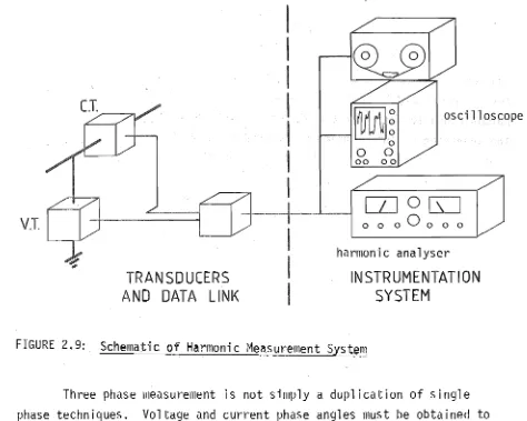
FIGURE 2.9: Schematic of Harmonic Measurement System

Three phase measurement is not simply a duplication of single phase techniques. Voltage and current phase angles must be obtained to a single reference angle, say red phase fundamental. The phase angle

at each harmonic in the Plessey instrument (Edward et al 1981) is the angle between the voltage and the current at that harmonic and thus no reference is possible. Although the instrumentation system of Breuer et al (1982) included a phase angle reference the phase information was

not as accurate as the magnitude, due to equipment resolution. The method of Crevier and Mercier (1978) was used and assumed a balanced system. Because this method gives only an approximate representation of an

unbalanced system the accurate three phase instrumentation with a dynamic range of 100 dB was not utilized to its potential. Although three phase measurement ,i s techni cally feas i b 1 e it has yet to be achi eved to a

14

Derivation of system impedance is an onerous task for a measurement system. It is not possible to obtain useful impedances with multiple sources on the system, a situation often encountered in practice. This is particular1y difficult below the 10th

harmonic due to the background harmonic levels (Kidd and Duke 1974). The injection of inter-harmonic frequencies by Baker (1981) avoids this problem but interpolation to harmonic frequencies is required. A range of harmonic impedances likely to be found with varying system configurations at each frequency is usually necessary. Often however, it is not possible to study the numerous outage conditions required (Huddart and Brewer 1966).

The ability of measuring equipment to determine accurate harmonic impedances is restricted. The cost of measurement is high and the

availability of suitable equipment and personnel is often limited.

Simulation can overcome these problems and reduce the need for measuring under varying system configurations and multiple source injection

conditions. With known or measured current injections from one source and measured voltages at one bus agreeing with simulated voltages at that bus, model results can be used at other locations with confidence. Using

measurement and modelling in this way reduces the need to measure simultaneously at large numbers of busbars; a daunting task.

2.6 MEASUREMENT AND MODELLING CORRELATION

An agreement between harmonic measurements on a system, and computer s-imulation of the same system, \l/ould confirm the validity of both the

measurement equipment and the computer model. However until this is achieved full confidence in both areas of endeavour cannot be guaranteed.

However, in dealing with a physical power system, it is not

possible to achieve exact agreement of modelled and measured quantities. The New Zealand Limits (New Zealand Electricity 1983)

specify the measurement accuracies necessary for the determination of the small signal levels usually associated with harmonics. They are:

the error in measuring constant harmonic ,current shall. not exceed 0.1% phase to earth system voltage.

The extent that present harmonic modelling meets quantitative accuracies can be assessed from the work of Owen et al (1980):

Resonant frequencies were predicted to within 5% of the measured values.

Magnitudes at resonance were predicted to within 50% of measured values.

- Magnitudes at frequencies not near a resonance were predicted to within 20% of measured values.

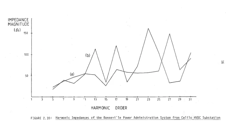
A second comprehensive study performed under EPR! guidance (Breuer et al 1982), on the Bonneville Power Administration System, produced the average measured and simulated impedances of Figure 2.10.

Both of these studies would be unacceptable if the above measurement limits "'Jere applied to modelling.

IMPEDANCE

MAGNITUDE

(n. )

150

100

50

3 5 7 9 11 13 15 17 19 21 23 25 27 29 31

HARMONIC

ORDER

FIGURE 2.10: Harmonic Impedances of the Bonneville Power Administration System from Celilo HVDC Substation (a) meas ured

CHAPTER 3

ALGORITHM DEVELOPMENT

3.1 INTRODUCTION

There is little difference in the basic approach to harmonic investigations when using either single or three phase models. However, the complexity and data requirements for three phase studies are much greater. Because of this the development of three phase software necessitates more effort on data preparation and output display.

Some early understanding of harmonic penetration was obtained in relation to HVDC convertors (Robinson 1966) and using analogue simulation. Laurent et al (1962), at the French end of the cross-channel HVDC link, found simulation results did not match those measured. System impedances were not accurately modelled and considerable imbalance between phases in measured voltages was reported. Brewer et al (1974) also reported

difficulty in matching predictive computer studies with measured results on the Kingsnorth HVDe scheme.

Digital computer models at harmonic frequencies have been

developed which have the capability to represent more of the elements of the transmission system. Campbell and Murray (1970), Kaban and Parten

(1970), Northcote-Green et al (1973a), Frosch and Schultz (1978), Mahmoud and Shultz (1982), and Breuer et al (1982) all used balanced transmission line parameters and loads, reducing the transmission system to a single phase positive sequence equivalent. Linear, passive elements allowed analysis at individual harmonic frequencies. Only the single phase model of Breuer et al (1982) has been used to compare harmonic impedances of a network with measured test data. There were frequencies where the

comparison was poor and again unbalanced impedances were reported.

Harmonic penetration studies have been undertaken for distribution systems, (Pileggi et al 1981 and McGranaghan et al 1981). In the former,

the low order unbalanced characteristic and non-characteristic harmonics were injected from a convertor load. Symmetrical component matrix analysis \Vas used to obtain harmonic voltages at specific network buses. In the

18

Kitchin (1981) proposed that a time domain solution using transient simulation would give accurate steady state harmonic levels where the

voltage waveform was affecting convertor current generation. This approach however does not include accurate transmission line frequency dependence. The ability of frequency domain techniques to allow this facility was a major reason for its use in this thesis.

This chapter describes an algorithm to model three phase harmonic penetration. An essential feature is that multiconductor trans~ission

1 i nes cannot be modelled with fundamenta 1 freq uency data. The algorithm encompasses convertor harmonic interaction as well as harmonic penetration modelling,and while the results being presented only relate to the latter~

the structuring of the programs has been made general to permit developments in both areas.

3.2 REQUIREMENTS FOR HARMONIC MODELLING

The requirements to be met for accurate harmonic modelling are:

transmission lines must be represented with provision for skin effect and standing wave phenomena.

load, transformer, generator, shunt capacitor and filter models should be included.

provision must be made for editing of data to allow for different system configurations.

nodal admittance matrices should be formed for a range of frequencies and not restricted to harmonic multiples of the fundamental.

it should be possible to calculate system impedances at any busbar.

the possibility of current injections at multiple locations in the system needs to be considered.

the network (assumed linear and passive) must be solved to obtain system voltages at all nodes for all frequencies.

line current flows should be calculated at each frequency.

These requirements utili$e standard power system techniques involving solution of simultaneous linear equations. Different

applications mean that not all the above features will be used in anyone study.

3.3 SINGLE PHASE MODELLING

The structure of the single phase algorithm is illustrated in Figure 3.1. This corresponds to the program ELAFANT (Baird 1981)~ used by New Zealand Electricity, and indicates the simplicity and efficiency of this software. Features of the program include:

fundamental frequency system component data is used at harmonic frequencies. This data is held in system data bases which means very little work is required in preparation for studies.

editing facilities can retain changes for future runs, i.e. only one set of data is needed which can easily be reconfigured for a desired system.

storage for a single admittance matrix only is required and this is reformed for each frequency.

Low. requirements for storage combined with efficient solution techniques and ease of data preparation makes the program fast and easy to operate. ELAFANT meets all the requirements of the previous section, except that of multiple injection locations, although this can be

performed if necessary by vector summation of the results of each separate injection.

FIGURE 3.1 Structure Diagram of Single Phase Modelling

Read Positive Sequence L-i ne Seri es

Impedance and Shunt Admit-tance for Fundamental Frequency from System Data Base

Read Balanced I,-oad, Trans-former.

~enerator.

Filter, and Shunt Data for Fundamental Frequency from System

~ata Base

Single Phase Harmonic Modelling

(ELAFANT)

Do Until Finished

Edit System for Required Changes Input Current Injection Busbar and Frequency Range

I

Form System Admittance Matrix Based on Simple

Functions of Frequency

I

Do For All Frequencies

I

Solve

[I] =

[Y][V]

to Obtain Positive Sequence Voltages and Output These

I

Calculate Line Current Flows and Output These

I

N

3.4 THREE PHASE ALGORITHM

Unbalanced transmission lines and to a lesser extent other system components, have led to the proposed development from single

phase to three phase analysis. The structure of the three phase algorithm developed is illustrated in Figure 3.2. The harmonic penetration program, HARMAC (abbreviation of AC HARMonics), is only one part of this diagram indicating that three phase modelling is not a direct extension of single phase techniques. This structure is however very similar to that used in three phase power flow studies.

Data preparation is not trivial in three phase harmonic modelling. Reasons for data complexity are:

unbalanced three phase load data.

three phase transmission line frequency dependence.

The volume of data and the need for practical program blocks are central to the algorithm developed; not speed or efficiency of computation as has been the case in development of power flow or transient stability simulation. The need for separate program blocks is a function of multiple use of software and practical program debugging and maintenance.

The first block of Figure 3.2, program TL (Transmission Line), calculates the transmission line parameters for each frequency over a required range using an Equivalent PI model. This is the subject of

Chapter 5. Program INTER (INTERactive) completes the data base by reading line data from TL in unformatted form and adding it to the unbalanced load and other component data required in the network. Use of unformatted data is a method of data compression to save storage. Both programs were obtained from New Zealand Electricity and extended from fundamental to harmonic frequencies. These two programs are unnecessary in single phase studies due to low data requirements and smaller software size. Data necessary for a network need not be reformed each time a study is contemplated.

FIGURE 3.2 Structure Diagram of Three Phase Modelling

From the line geometry, gro resistivity. conductor, type and l"j ne length calculate the series impedance and shunt admittance matrices for all frequencies and lines

(TL)

Three Phase Harmonic Modelling

Form dataset using shunt capacitors,

transformers, ge"nerators, filters and unbalanced loads at

fundamental frequency and line data for all frequencies

(INTER)

I

Read data, and form into admittance matrices for all frequencies. Solve for harmonic voltages, currents and impedances.

(HARMAC)

NOTE: Program name is in brackets

Plot voltages, currents and impedances.

(GRAPHl)

The data flow diagram of Figure 3.3 indicates the individual programs and major data files that form the basis of the three phase steady state solution technique. Data formation for both the harmonic penetration software, and three phase power flow (Harker and Arrillaga 1979) is performed by the same software. This ensures that the system configuration used to supply data to program HARMCO (COnvertor HARi>1onics) by the harmoni c penetrati on and power fl ow programs is the same. It

also avoids the duplication of data preparation softv/are, particularly for the transmission lines where similar analysis techniques can be used for fundamental and harmonic frequencies. The disadvantage of this structure is that line data for all the desired frequencies needs to be stored as data for HARMAC.

The three phase AC/DC power flow supplies fundamental frequency data and the convertor operating state (Harker 1980) to the convertor interaction software, HARMCO. This software uses the three phase

FIGURE 3.3 Data Flow Diagram

Conductor Data

Transmission Line Parameter Program

(TL)

Line

geometry and conductor type data

NOTE: Program name in brackets

Interactive Data Program

(INTER)

Generator, transformer shunt, filter and load data

Harmonic

Penetration Program (HARMAC)

Convertor Interactio Program

(HARMAC)

Power Flow Program (PF)

Graphics Program (GRAPHl)

o

3.5 THREE PHASE HARMONIC PENETRATION

The three phase harmonic penetration program HARMAC is illustrated in the structure diagram of Figure 3.4. Features of the algorithm include:

three phase mutually coupled transmission line data can be utilized.

three phase unbalanced loads and other system components are mode" ed.

separate admittance matrices are formed for each frequency.

three phase impedance matrices for a reduced portion of the network suitable for filter design or convertor interaction studies are derived.

unbalanced current injections at a number of busbars on the system can be specified.

All the requirements previously stated for harmonic modelling have been met, although data file editing is not comprehensive.

For a three phase network, unbalanced self and lllutual admittances of network elements can be modelled as well as circuit coupling. As indicated earlier, it is assumed that the AC system is linear and passive and therefore the principle of superposition may be applied to enable each harmonic to be considered independently. '

In a multibranch interconnected network an admittance matrix

[vhl is formed from the individual elements, for each particular harmonic, h. Harmonic currents are injected into the buses under consideration and the voltages throughout the system calculated from the solution of:

=

For the three phase system, the elements of the admittance matrix are themselves 3x3 matrices consisting of self and transfer admittances. Figure 3.5 indicates the nature of the analysis where h sets of linear

FIGURE 3.4 Structure Diagram of Three Phase Harmonic Penetration Program

Input frequency range and harmonic impedance busbars.

I

• capacitors, transformers, generators, filters and unbalanced loads at fundamental frequency and form into admittance matri ces.

Read 1 i ne data for all frequencies and include in harmonic admittance matrices.

Harmonic Penetration Program

(HARt1AC)

Calculate system harmoni c. impedance matrix for a reduced system.

Input current injection bus bar and three phase injection data.

Solve

[IhJ = [Y h]

~~

for all frequencies to get three phase

vo ltages and output.

FIGURE 3.5. Solution of h}Linear Simultaneous Eguations

lAlhile it is usual to consider harmonic frequencies any frequencies may be solved for.

The injected currents at most AC busbars will be zero, since the sources of the harmonics considered are generally from static convertors.

I

las~

(Zollenkopf 1970), using row ordering techniques to reduce the amount of off-diagonal element build-up. The matrix is triangulated using Gaussian elimination, down to but excluding the rows of the specified buses.

The resulting matrix equation for an n-node system with n-j+1 injection points is

o

o

I. \

J

I n

=

Y ..

JJ 0

Y •

nJ

• •• Y •

In

••• Y

nn

V. 1

J-V.

J

/J }

As a consequence, I j ... In remain unchanged since the currents above these in the current vector are zero. The reduced matrix equation is:

I . J

=

Y ..

JJ

Y .

nJ Y nn

V.

J

V n

(3.3)

where the admittance matrix is of order equal to 3 times the number of injection busbars. The elements are the self and transfer admittances of the reduced system as viewed from the injection busbars. An impedance matrix may be obtained for the reduced system by matrix inversion.

Reducing a system to an equivalent impedance matrix is not only useful for filter design where the system as viewed from one bus is required, but also where a number of convertors are connected to the AC system at different points, Figure 3.6. In this case the reduced

admittance matrix would be of order 9.

Convertor 1

AC

System

Convertor 2

FIGURE 3.6 Three Convertors Attached to Different Busbars on the AC System

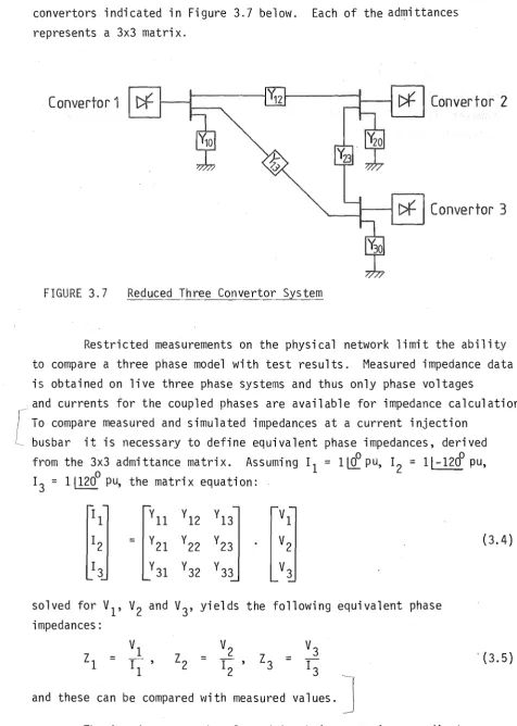
convertors indicated in Figure 3.7 below. Each of the admittances represents a 3x3 matrix.

Convertor 1

r - - - - 1 - - J

t:f

Con ver to r 2

Convertor 3

FIGURE 3.7 Reduced Three Convertor System

Restricted measurements on the physical network limit the ability to compare a three phase model with test results. ~1easured impedance data is obtained on live three phase systems and thus only phase voltages

and currents for the coupled phases are available for impedance calculations. To compare measured and simulated impedances at a current injection

bus bar it is necessary to define equivalent phase impedances, derived from the 3x3 admittance matrix. Assuming

13 = 111200 pu, the matrix equation:

o 0

II

= lLQ:

=

II Y_ll Y₁₂ Y₁₃ VI

12 = Y21 Y22 Y23 _V

2 (3.4)

13 Y _{31 Y32 Y 33} V3

solved for VI' V2 and V 3' yields the fo 11 owi ng equivalent phase impedances:

ZI

=

Z2 = V₂

Z3

V3

' (3.5)

~

12

,

=

13

I _'I

and these can be compared with measured values.

J

3.6 FORMATION OF THE NODAL ADMITTANCE MATRICES 3.6.1 Introduction

To enable harmonic penetration analysis to be performed it is necessary to form a mathematical representation of the power system. However,the electrical characteristics of an interconnected network are extremely complex. By considering the individual physical elements the parameters of which can be determined and connecting them in the manner of the physical network, this complexity can be overcome. Nodal

admittance matrix techniques are presented to perform this interconnection efficiently.

Phase quantities are retained throughout the formation and solution of the harmonic admittance matrices. Symmetrical components provide no computational advantage and are only used as an aid to interpretation of resul ts.

This s~ction treats ihe interconnection of various three phase element types by the use of linear transformation techniques. It is left to the two succeeding chapters to assign the physical elements of the network to these element types.

Admittance matrices for each frequency have the same non-zero elements with values determined by element models.

3.6.2 Network Subdivision

Although an element, or branch, of a network is the basic component elements may be coupled and non-homogeneou~ i.e. mutually coupled

transmission lines with different tower geometries over the line length. To facilitate the inclusion of this a subsystem is defined as follows:

A subsystem is the unit into which any part of the system may be divided such that no subsystem has any mutual coupling between its constituent branches and those of the rest of the system.

The smallest unit of a subsystem is a single network element.

The subsystem unit is retained for input data organisation. Data for any subsystem is input as a complete unit, the subsystem admittance matrix is formulated and then combined in the total system admittanc~

Subsystem admittance matrices may be derived bf finding. for

each section. the ABCD or transmission parameters, then combining these by matrix multiplication to give the resultant transmission parameters. These are then converted to the required nodal admittance matrices.

This procedure involves an extension of the usual two port network theory to multi-two-port networks. Currents and voltages are now matrix quantities as defined in Figure 3.8. Dimensions of the parameter matrices correspond to those of the section being considered, i.e. 3,6,9, or 12 for 1, 2, 3 or 4 mutually coupled three phase

elements respectively. All sections must contain the same number of mutually coupled three phase elements, ensuring that all the parameter matrices are of the same order and that the matrix multiplications are executable. Uncoupled elements need to be considered as coupled ones with zero coupling to maintain correct dimensions for all matrices.

Once the resultant ABCD parameters have been found the equivalent nodal admittance matrix for the subsystem can be calculated from:

[YJ

I[DJ~~ ~

[ [BJ- 1

I I

I

-

,-[c] -

[OJ [8J-1

_[B]-l [A]

(b) Multi-two port network

(a) Matrix transmission parameters FIGURE 3.8 Two Port Network

32

Two-port network theory is not the only way a number of sections can be reduced to a branch equivalent. Matrix reduction introduced for systems impedance calculation in the previous section could also have been used (Alvarado 1982).

3.6.3 Linear Transformation

Linear transformation techniques enable the admittance matrix of any network to be found in a systematic manner (Kron 1965 and Brameller et al 1969). Steps needed to form the network admittance matrix by linear transformation are:

label the nodes in the original network.

number in any order the branches and branch admittances.

form the primitive network admi ttance matrix [Vpr"illl] by inspection.

form the connection matrix

[cl

calculate the element nodal admi ttance matrix using [Vabc] = [CJT [VprinJ

[c]

Examples of this techniqu~ can be found in Harker (1980).

Representation of three phase elements by the use of compound admittances will be used extensively. Formation of both the primitive and actual network admittance matrices using three phase compound admittances is covered in deta"il in Arr"illaga et al (1983a).

For the models dev~loped in this section, the intermediate steps in forming the element nodal admittance matrices have been neglected, similar to the program implementation.

3.6.4 Shunt and Series Elements

k

I~

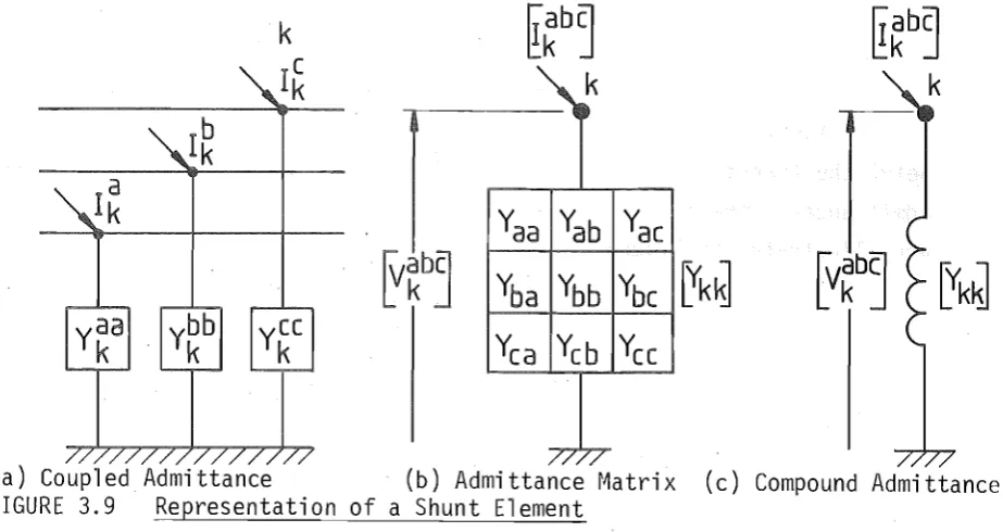
(a) Coupled Admittance (b) Admittance Matrix (c) Compound Admittance FIGURE 3.9 Representation of a Shunt Element

The admittance matrix is usually diagonal as there is normally no coupling between the components of each phase. It is incorporated directly into the system admitta~ce matrix, contributing only to the self admittance of the particular bus. Shunt elements represent the simplest subsystem, being composed of only one busbar.

Coupled series admittances between busbars i and k in Figure 3.10 reduce to the'nodal admittance matrix and compound admittance indicated.

I~

I

_yaa

ik

I~

_ybb

ik

IS

I

I~

(a) Coupled

(b) Adm; ttance r1atri x

(c) Compound Admittance

3.6.5 Coupled Shunt Elements

T\l1O three phase shunt branches coupled together, a common exampl e being the transformer, may be represented using two coupled compound

admittances. The admittance matrix and compound admittance representation are illustrated in Figure 3.11.

(a) Admittance Matrix

(b) Compound Admittance

FIGURE 3.11 T~<Jo ~~inding Three Phase Transformer asTwg" Coupled Compound Admi.tt(inces

It should be noted that:

as the coupling between the two compound admittances is bilateral.

Practical details of the different coupling arrangements possible are discussed in Laughton (1968) and Dillon and Chen (1972).

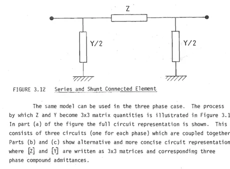
3.6.6 Combined Series and Shunt Connected Elements

(3.7)

For this element representation in single phase analysis, the usual example being the transmission line, half of the total shunt admittance is connected to earth at each terminal and the series