Maximum Likelihood Estimation of the Parameters of Exponentiated Generalized Weibull Based on Progressive Type II Censored Data

http://www.scirp.org/journal/ojs ISSN Online: 2161-7198

ISSN Print: 2161-718X

DOI: 10.4236/ojs.2017.76067 Dec. 6, 2017 956 Open Journal of Statistics

Maximum Likelihood Estimation of the

Parameters of Exponentiated Generalized

Weibull Based on Progressive

Type II Censored Data

Ibrahim Sawadogo

1

, Leo Odongo

2

, Ibrahim Ly

3,4

1_{Pan African University Institute of Science, Technology and Innovation, Nairobi, Kenya} 2_{Department of Statistics and Actuarial Science, Kenyatta University (KU), Nairobi, Kenya}

3_{Department of Mathematics, University of Ouagadougou, Ouagadougou, Burkina Faso} 4_{Department of Mathematics, University of Potsdam, Potsdam, Germany}

Abstract

The Exponentiated Generalized Weibull distribution is a probability distribu-tion which generalizes the Weibull distribudistribu-tion introducing two more shapes parameters to best adjust the non-monotonic shape. The parameters of the new probability distribution function are estimated by the maximum likelih-ood method under progressive type II censored data via expectation maximi-zation algorithm.

Keywords

Maximum Likelihood, Type II Censored Data, Exponentiated Generalized Weibull, EM-Algorithm

1. Introduction

Various probability density functions have been proposed to perform statistical analysis of lifetime data. The Weibull distribution is one of the most widely used distributions in the analysis of lifetimes data. It was introduced by the French Mathematicians Fréchet (1928) [1]. Indeed in the 1920s Fréchet developed a distribution to which he gave his name; Fréchet distribution, as an extreme value distribution. This distribution is in fact equal to the reciprocal of the Weibull distribution. Rosin and Rammler (1933) [2] applied Fréchet’s ditribution to describe the particle size distribution generated by grinding, milling and crushing operations of materials. This probability distribution has been widely

How to cite this paper: Sawadogo, I., Odongo, L. and Ly, I. (2017) Maximum Likelihood Estimation of the Parameters of Exponentiated Generalized Weibull Based on Progressive Type II Censored Data. Open Journal of Statistics, 7, 956-963.

https://doi.org/10.4236/ojs.2017.76067

Received: October 10, 2017 Accepted: December 3, 2017 Published: December 6, 2017

Copyright © 2017 by authors and Scientific Research Publishing Inc. This work is licensed under the Creative Commons Attribution International License (CC BY 4.0).

http://creativecommons.org/licenses/by/4.0/

DOI: 10.4236/ojs.2017.76067 957 Open Journal of Statistics used as a probabilistic model in studies on lifetimes. Mudholkar and Srivastava (1993) [3] introduced the exponentiated Weibull distribution to analyse bathtub failure rate data which cannot be handled well by the regular Weibull for monotonicity of its hazard rate. Also Zhang and Xie (2011) [4] worked on bathtub failure data using the truncated Weibull distribution. Soumaya and Soufiane (2014) [5] have given estimation of the parameters of the exponentiated Weibull distribution and the additive Weibull distribution, which are two specific generalizations of the Weibull distribution.

Cordeiro, et al. (2013) [6] introduced the exponentiated generalized class of distribution which is more general than the two classes of Lehmann’s (1953) [7]

alternatives, it is a combination of the Lehmann type I and type II alternatives. Indeed, for any baseline (or parent) distribution it is possible to define the corresponding Exponentiated Generalized family of distribution. Cordeiro, et al. (2013) discussed four special models namely the Exponentiated Generalized Fréchet, the Exponentiated Generalized Normal distribution, the Exponentiated Generalized Gamma distribution and the Exponentiated Generalized Gumbel distribution. Oguntunde et al. (2015) [8] have discussed the special case of the Exponentiated Generalized Weibull distribution by using the Weibull distribution as baseline distribution. The proposed distribution has four parameters (three shape parameters and one scale parameter). The work of Oguntunde et al. is mainly focused on the mathematical properties of the distribution like the moments, the limiting behaviour of the functions (pdf and cdf), the reliability analysis, and the quantile function.

The probability density function and the cumulative distribution function of the Exponentiated Generalized Weibull are respectively given by:

(

)

1

{ }

( )

{ }

( ) 1

; , , , e 1 e

b

a a

x x

x

f x a b ab α α

α

β β

α

α β

β β

− −

− −

   

= _{  } − _

 

  (1)

and

(

)

{ }

( )

; , , , 1 e

b a x

F x a b

α β

= −_ − βα _

  (2)

where x>0, a>0,

b

>

0

, α>0,

β

>0.

The Exponentiated Generalized Weibull generalizes the following distributions:

For a=1, Generalized Weibull; For

b

=

1

, Exponentiated Weibull; For

a

= =

b

1

, Weibull distribution; For

a

= = =

b

α

1

, Exponential distribution.

The survival function and the hazard function have respectively the following expressions:

(

)

(

)

{ }

( )

; , , , 1 ; , , , 1 1 e

b a x

S x a b

α β

= −F x a b

α β

= − −_ − βα _

  (3)

DOI: 10.4236/ojs.2017.76067 958 Open Journal of Statistics

(

)

( )

{ }

{ }

( )

( )

{ }

1 1

e 1 e

; , , ,

1 1 e

b

a a

x x

b a x

x ab

h x a b

α α

α

α

β β

β

α β β α β

− −

− −

−

 

  ₋

   

   

=

 

− −_{ }

 

(4)

2. Parameters Estimation

2.1. The Model

Let us assume that we have n independent variables in a trial, and the ordered m failures are observed under the progressive type-II censoring plan R=

(

R1,,Rm

)

,

where Rj≥0 for j=1,,m and 0

m j j= R + =m n

∑

. Let the observed and censored data be respectively Y=

(

Y1,,Ym

)

and Z =

(

Z1,,Zm

)

, where

(

1, , j

)

j j jR

Z = Z  Z for j=1,,m . Now consider X=

(

Y Z,

)

to be the

complete data (observed and censored data together). Then the joint probability that the complete sample (the complete data likelihood) is observed is given by

(

)

(

)

(

)

1 1

, , , , , , , , , , , ,

j

R m

c j jk

j k

L x a b

α β

f y a b

α β

f z a b

α β

= =

 

=  

 

∏

∏

(5) (Ng et al 2002) [9].

From which we get the following log-likelihood by substituting in (5) the pdf by expression (1)

(

)

(

)

(

)

( )

(

)

(

)

( )

1

1 1

1 1 1 1

1 1

log , , , ,

log log log log 1 log

1 log 1 e

1 log

1 log 1 e

j

j j

j

jk c

m j

j

a

m m

y j

j j

R R

m m

jk jk

j k j k

a R

m

z

j k

L x a b

y

n a n b n n

y

a b

z z

a

b

α

α

α

β

α

β

α β

α β α

β

β

α

β β

=

−

= =

= = = =

−

= =

 

= + + − + − _{ }

 

 

   

−   + −  −  

 

 

  _{ }

   

+ − _{ }− _{ }

   

 _{ }

+ −  − 

 



∑

∑

∑

∑∑

∑∑

∑∑



 _

(6)

2.2. EM Algorithm

2.2.1. E-Step

In oder to tackle the E-step the conditional expectation of the log-likelihood given the observed sample Y=

(

y y1, 2,,ym

)

is computed. Let us denote it by

( )

Q θ where θ=

(

a b, , ,α β

)

is the vector of parameters. That is,

( )

(

log c

(

, |

)

)

Q θ =θ L X θ Y

The conditional expectation of the above log-likelihood becomes

( )

(

)

(

)

( )

1

1 1

log log log log 1 log

1 log 1 e j

m j j

a

m m

y j

j j

y

Q n a n b n n

y

a b

α

α

β

θ α β α

β

β

=

−

= =

 

= + + − + − _{ }

 

 

   

−   + −  −  

 

 

  _{ }

∑

DOI: 10.4236/ojs.2017.76067 959 Open Journal of Statistics

(

)

(

)

( ) 1 1 1 1 1 1

1 log |

|

1 log 1 e |

j j j jk R m jk jk j j k R m jk jk j j k a R m z jk j j k z z y z

a z y

b z y

α θ α θ β θ α β β = = = = − = =    

+ − _   > _

 

 

_{ } 

 

− _{ } >

_{ } 

 

  _{ }  

 

+ − _  −   > _

       

∑∑

∑∑

∑∑

   (7)

Thus, to facilitate the E-step, the conditional distribution of Z for given Y and the current value of the parameters, needs to be determined.

The conditional distribution of Z for given Y is given by

(

)

(

(

)

)

| , | , , 1 , jk

Z Y jk jk j

j

f z

f z Y y z y

F y

θ

θ

θ

= = >

−

(8)

see Ng et al. (2002). Let us set

(

, _j

)

log zjk | _{jk j}

A θ y _θ z y

β

   

= _   > _

 

 



(9)

(

, _j

)

zjk | _{jk j}

B y z y

α θ θ β _{ }   

= _{ } >

_{ }     (10) and

(

)

( ) ,

log 1 e jk |

j a z jk j C y z y α β θ θ −   _{ }    

= _  −   > _

 

 

 

 

 (11)

Using (8)-(11) the expressions for A

(

θ,yj

)

, B

(

θ,yj

)

and C

(

θ,yj

)

become

(

)

(

)

( )

(

(

)

)

( )( )

(

)

(

)

(

)

1 0 log 1

, 1 e

1

1 ,

0, 1

j a v y j v j v j j y b ab A y

v a v

F y

a v y

α β α β θ α α θ β ∞ _{− +} =  −   _ = _{ } − +  −    _    

+ Γ +

 

∑

(12) where

( )

1

0, e dz

c

c ∞ − −z z

Γ =

∫

is the upper incomplete gamma function.

(

)

(

)

(

( )

(

)

)

(

(

)

(

)

)

( 1)( ) 2

0

,

1 1

1 1 e

1 , 1

j

j

v

a v y j v j B y b ab

a v y

v

F y a v

DOI: 10.4236/ojs.2017.76067 960 Open Journal of Statistics

(

)

(

)

(

( )

)

( 1)( )

0 0 1 1 , e 1 1 , j v

a v i y j i v j b ab C y v ia v i

F y α β

θ

θ

∞ ∞ _{− + +} = = − −   = − _{ } + +  −   

 

∑∑

(14)

We therefore obtain an expression for the conditional expectation of the log- likelihood as

( )

(

)

(

)

( )

(

)

(

)

(

)

(

)

(

)

1 1 1

1 1 1

log log log log 1 log

1 log 1 e

1 , , 1 ,

j m j j a m m y j j j

m m m

j j j j j j

j j j

y

Q n a n b n n

y

a b

R A y a R B y b R C y

α

α

β

θ α β α

β

β

α θ θ θ

= − = = = = =   = + + − + − _{ }         −   + −  −           + − − + −

∑

∑

∑

∑

∑

∑

(15)

where the functions A, B, and C are respectively defined in (12)-(14).

2.2.2. M-Step

In the M-step on the p-th iteration of the EM algorithm, the value of θ which maximizes

(

( 1)

)

, p

Q

θ θ

− will be used as the next estimate θ( )p of θ. Where ( )p

(

( ) ( )p _, p_, ( )p_, ( )p

)

a b

θ

=

α

β

_{is the vector of parameters at the p-th iteration}

1

p≥ , and

θ

( )0 =

(

a( ) ( )0,b0,

α

( )0,

β

( )0

)

is the initial value of the vector of

parameters.

( )

(

1

)

(

(

)

( 1)

)

, p log c , | , p

Q

θ θ

− =θ L X

θ

Y

θ

−

Therefore, if at the p-th stage the estimate of θ is θ(p−1)_{, then} θ( )p _{can be} obtained by maximizing

( )

(

)

(

)

(

)

( )

(

)

(

( )

)

(

( )

)

(

)

(

( )

)

1 1 1 1 1 1 1 1 1 1

, log log log log 1 log

1 log 1 e

1 , ,

1 , j m j p j a m m y j j j m m p p

j j j j

j j m p j j j y

Q n a n b n n

y

a b

R A y a R B y

b R C y

α

α

β

θ θ α β α

β

β

α θ θ

θ − = − = = − − = = − =   = + + − + −           −   + −  −         _{ } + − − + −

∑

∑

∑

∑

∑

∑

(16)

Then _θ( )p _{is solution of the following system of equations}

( )

(

)

( )

(

)

( )

(

)

( )

(

)

1 1 1 1 , 0 , 0 , 0 , 0 p p p p Q a Q b Q Q θ θ θ θ θ θ α θ θ β − − − − ∂ = ∂ ∂ = ∂ ∂ = ∂ ∂ = ∂ (17)

DOI: 10.4236/ojs.2017.76067 961 Open Journal of Statistics

(

)

( ) ( ) ( )

(

)

( )

(

( )

)

(

)

1

1 1 1

1

1 1

1 1

1

e

1 , 0

1 e

log 1 e , 0

log log log 1 j j j a y j

m m m

j p

j j

a

j j y j

a m m y p j j j j m m

j j j

j j j m j y y n

b R B y

a

n

R C y

b

y y y

n a y a b α α α α β α β β α β θ β θ

α β β β

β − − = = − = − − = = = = =               − _{ } + − − =     _{− }     _{ }  +  −  + =             + _{ }− _{   }       + −

∑

∑

∑

∑

∑

∑

∑

∑

( ) ( ) ( )

(

)

(

)

(

)

( ) ( ) 1 1 1 1 e , 0 1 e e 1 1 0 1 e j j j j a y j m p j j a j y a y j m m j a

j j y

y

R A y

y

y

n m a a b

α α α α α β β α β α β β θ β

α α α

β β β β

− − = − − = = −                _{    }  _{    }       _{+ =}     _{−  }  _{ }        _{+ −   −}         − + _{ } − =  _{   }  _{−  }    

∑

∑

∑

(18)

From the second equation in the above system we can express ( )p

b for known ( )p

a , α( )p ,

β

( )p as: ( )

( )

(

)

( ) ( )

(

( 1)

)

1 1

log 1 e ,

p p p j p a

m _y m

p

j j

j j

n b

R C y

α β θ − ₋ = = = −  _{ }   ₋  ₊        _{ }   

∑

∑

(19)

The expressions for ( )p

a , α( )p and

β

( )p are not available in closed form.

The solution to the M-step does not exists in closed form. For this case Dempster et al. (1977) [10] defined what is called the generalized EM algorithm (GEM algorithm) for which the M-step requires _θ( )p

to be chosen such that ( ) ( )

(

1

)

(

( 1) ( 1)

)

, ,

p p p p

Q

θ

θ

− ≥Q

θ

−

θ

−

(20) Since we need only to increase the likelihood, we may replace the M-step with a single iteration of the Newton-Raphson (N-R) algorithm.

3. Simulation

3.1. Simulation

For the simulation the M-step is replaced by a single iteration of the Newton- Raphson algorithm.

For the values of n=30 and m=20 and θ=

(

1,1,1,1

)

progressively Type-

II censored sample was generated from the Exponentiated Generalized Weibull distribution using the algorithm in Balakrishnan and Sandhu (1995) [11].

The algorithm is defined as follows:

DOI: 10.4236/ojs.2017.76067 962 Open Journal of Statistics

• Set 1(i Rm Rm1 Rm i1)

i i

V =W + + −+ + − + for

i

=

1, 2,



,

m

• Set Ui = −1 V Vm m−1Vm i− +1 for

i

=

1, 2,



,

m

. Then U U1, 2,,Um is the

required progressive Type-II censored sample from the Uniform (0, 1) distribution.

• Finally, we set 1

(

)

,

i i

X =F− U

θ

for

i

=

1, 2,



,

m

, where 1

( )

.,

F−

θ

is the inverse cdf of the Exponentiated Generalized Weibull distribution. Then

1, 2, , m

X X  X is the required progressive Type-II censored sample from the Exponentiated Generalized Weibull distribution.

with censoring scheme R=

(

1, 3,1,1,1,1,1, 0, 0, 0, 0,1, 0, 0, 0, 0, 0, 0, 0, 0

)

.

The generated sample is:

0.0138 0.0230 0.0447 0.2401 0.3091 0.3264 0.4597 0.5448 0.5841 0.7274 0.9875 1.1164 1.2090 1.3519 1.4896 1.5041 1.6224 2.9952 3.4537 3.6385 Via the EM algorithm discussed in Section 2, the computed MLEs of the parameters become:

ˆ

0.7606

a

=

, bˆ=0.8272,

α

ˆ

=

1.0911

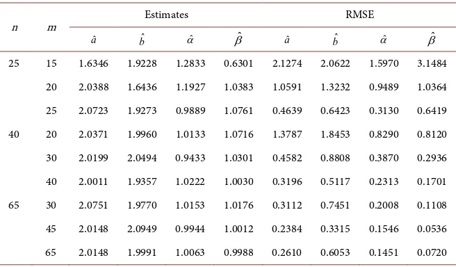
and _βˆ_=1.0365

In Table 1 a Monte Carlo simulation for N = 500 was used to compute the RMSE and the mean estimates for different value of n, m and θ=

(

2, 2,1,1

)

. The

following formula was used to compute the RMSE

( )

(

)

2

1

ˆ ˆ

RMSE

N _i i N

λ λ

λ

=

−

=

∑

where ˆ

i

λ is the i-th estimates of the parameter λ

3.2. Remarks

• For fixed sample size n and by increasing m, we get smaller RMSE’s.

• By increasing the sample size n, we get smaller RMSE’s.

[image:7.595.210.538.532.724.2]

• The largest values of m in each case represent the complete sample case.

Table 1. RMSE of the estimators.

n m Estimates RMSE

ˆ

a _bˆ αˆ _βˆ _{aˆ b}ˆ αˆ _βˆ

25 15 1.6346 1.9228 1.2833 0.6301 2.1274 2.0622 1.5970 3.1484

20 2.0388 1.6436 1.1927 1.0383 1.0591 1.3232 0.9489 1.0364

25 2.0723 1.9273 0.9889 1.0761 0.4639 0.6423 0.3130 0.6419

40 20 2.0371 1.9960 1.0133 1.0716 1.3787 1.8453 0.8290 0.8120

30 2.0199 2.0494 0.9433 1.0301 0.4582 0.8808 0.3870 0.2936

40 2.0011 1.9357 1.0222 1.0030 0.3196 0.5117 0.2313 0.1701

65 30 2.0751 1.9770 1.0153 1.0176 0.3112 0.7451 0.2008 0.1108

45 2.0148 2.0949 0.9944 1.0012 0.2384 0.3315 0.1546 0.0536

DOI: 10.4236/ojs.2017.76067 963 Open Journal of Statistics

4. Conclusion

The parameters of the Exponentiated Generalized Weibull distribution were estimated using maximum likelihood estimation method via Expectation Maximization (EM) algorithm. The Root Mean Square Error were computed at different values of the sample size n and failures (observed data) m. It was observed that the RMSEs were smaller for fixed sample size n and increasing the size m of the observed data, and also for the increasing sample size n.

Acknowledgements

I would like to thank my supervisors Professor Leo Odongo and Doctor Ibrahim Ly for accompanying me through this work. Sincere thanks to the African Union for giving me the opportunity to do scientific reseach.

References

[1] Fréchet (1928) Sur la loi de probabilité de l'écart maximum. Annales de la societe Polonaise de Mathematique, 6, 93-116

[2] Rosin, P. and Rammler, E. (1933) The Laws Governing the Fineness of powdered coal. Journal of the Institute of Fuel, 7, 29-36.

[3] Mudhokar, G.S. and Srivastava, D.K. (1993) Exponentiated Weibull Familly for Analysing Bathtub Failure-Rate Data. IEEE Transaction on Reliability, 42, 299-302.

https://doi.org/10.1109/24.229504

[4] Zhang, T. and Xie, M. (2011) On the Upper Truncated Weibull Distribution and Its Reliability Implications. Reliability Engineering and System Safety, 96, 194-200.

https://doi.org/10.1016/j.ress.2010.09.004

[5] Soumaya, G. and Soufiane, G. (2014) Parameters Estimations for Some Modifica-tion of the Weibull DistribuModifica-tion. Open Journal of Statistics, 4, 597-610.

https://doi.org/10.4236/ojs.2014.48056

[6] Cordeiro, G.M. Ortega, E.M. and Da Cunha, D.C. (2013) The Exponentiated Gene-ralised Class of Distributions. Journal of Data Science, 11, 127.

[7] Lehman, E.L. (1953) The Power of Rank Tests. The Annals of Mathematical Statis-tics, 24, 23-43. https://doi.org/10.1214/aoms/1177729080

[8] Oguntunde, P., Odetunmibi, O. and Adejumo, A. (2015) On the Exponentiated Generalized Weibull Distribution: A Generalization of the Weibull Distribution. Journal of Science and Technology, 8, 1-7.

[9] Ng, H.K.T., Chan, P.S. and Balakrishnan, N. (2002) Estimation of Parameters from Progressively Censored Data Using EM Algorithm.Computational Statistics & Data Analysis, 39, 371-389. https://doi.org/10.1016/S0167-9473(01)00091-3

[10] Dempster, A.P., Laird, N.M. and Rubin, D.B. (1977) Maximum Likelihood from Incomplete Data via the EM Algorithm. Journal of the Royal Statistical Society, Se-ries B, 1-38.