Pragmatic optimisation methods for determining material constants of viscoplasticity model from isothermal experimental data

Pragmatic optimisation methods for determining the material constants of

a visco-plasticity model from isothermal experimental data

J. P. Rouse1*, C. J. Hyde1, W. Sun1, T. H. Hyde1

1_{Department of Mechanical, Materials and Manufacturing Engineering}

University of Nottingham, Nottingham NG7 2RD UK

*Corresponding Author - Email:[email protected], Telephone:+44 (0) 115 84 67683

Abstract

A procedure to estimate material constants for the unified Chaboche visco-plasticity model from experimental data has been published elsewhere 1, 2; however several critical

assumptions are made to enable this. Pragmatic optimisation is therefore required to determine the material properties more accurately and efficiently in light of the complex deformation mechanisms and their interactions. Automation is critical due to the large amounts of data generated in testing. Complications that inhibit this process can arise due to factors such as experimental scatter. In this paper, a general optimisation framework is discussed and investigated using data from isothermal tests on a P91 steel at 600°C. Potential obstacles in the procedure are addressed and solutions (such as pre-optimisation experimental data “cleaning”) are suggested.

Keywords: Chaboche; Visco-Plasticity Model; Low Cycle Fatigue; Optimisation; P91.

1

Introduction

High temperature components, such as steam pipe work used extensively in the power and petrochemical industries or turbine blades in aero engines, may inevitably experience not only fluctuations in loading but also in operating temperature. These fluctuations may be periodic or cyclic in nature. Additionally, focusing particularly on the future trends of power plant operation, these fluctuations will become more pronounced as operators attempt to generate in a highly strategic manner, maximising generation effectiveness 3, 4. Variations in loading or temperature present serious complications when analysing such components due to the cyclic hardening behaviour of materials if the material works within the plastic range. Models that can predict this behaviour, while allowing for the creep response to be included as well, are therefore of great interest to many industries. Approximate component analysis methods, such as those used in the well-known R5 procedure for creep fatigue interaction, can estimate these effects however in some cases full inelastic analysis may be required 5, 6. With greater predictive accuracy, power generation plant, for example, could be operated with confidence in a more arduous fashion, potentially allowing for greater plant flexibility.

In this paper, the Chaboche visco-plasticity model will be implemented to describe complex visco-plasticity behaviour 7. An effective optimisation procedure for determining the material constants in the model is described. This procedure utilises isothermal uniaxial cyclic

Given some initial yield condition, isotropic and kinematic hardening may occur under sufficient loading. Isotropic hardening causes the uniform expansion of the yield surface 1, 2, 8,

9_{, while kinematic hardening will not affect the size of the yield surface, but cause an offset in}

some direction and affect its orientation 2, 8, 9_.

2

The Chaboche Unified Visco-Plasticity Model

The Chaboche model decomposes total strain into elastic and plastic components,

incorporating the evolution of both kinematic and isotropic hardening, through the use of appropriate internal variables (χ and R, respectively). The uniaxial form of the Chaboche model is used to illustrate the optimisation procedure described in this paper. Nonlinear hardening is estimated through the use of several differential equations that update the relevant internal variables. In this way, only one yield surface definition is required 7, 10, as opposed to other methods such as the Mroz model 11. For the Chaboche model, the yield function is defined by equation (1) 7, 12.

0

f =s c- - - £R k (1).

The back stress (χ) designates the centre of a yield surface and the drag stress (R) denotes the variation of its size from its initial size, k7. For equation (1), it can be seen that when f has a value less than or equal to 0, the stress point (σ) must lie within the yield surface, indicating elastic deformation only. To provide a better approximation of kinematic effects, the back stress can be decomposed into several components 7, 10 (note in the present study, a two back stress component model was found to be satisfactory 2). An Armstrong and Frederick type kinematic hardening law is used to define the increment for each back stress component, taking the form of equation (2) 1_{. By decomposing the back stress into multiple components,}

transient and long term behaviour may be described 13. The total back stress is given as the summation of these components; therefore for m components of back stress, the total back stress (χ) is given by equation (2).

(

)

1 , m p

i i i i i

i

dc C a de cdp c c

=

= - =

å

where ai and Ci are both material constants (Ci dictates how quickly the stationary value ai is achieved with increasing plastic strain 1, 14_{). The accumulated plastic strain (p), on which}

most of the internal variables are dependent, is a monotonically increasing quantity and is the summation of the modulus of the plastic components of total inelastic strain (εp), or described mathematically in equation (3) 2. The effects of isotropic hardening are represented by the scalar drag stress (R). As such, R will alter only the size of the yield surface; it’s evolution controlled by equation (3) [1]. In this form, the drag stress will undergo some initial

monotonic increase before reaching a stabilised asymptotic value (Q) 1, 2, 14, 15. Creep effects will be present when time or strain rate have an influence on inelastic behaviour 7. This is accounted for through the definition of a viscous stress, σv, assumed to take the form of a power law 7 such as equation (4), where Z and n are viscous material coefficients. The viscous stress, along with the kinematic and isotropic internal variables, defines the total stress (σ) given in equation (4).

(

)

, p

1/

( )sgn( ), n

v v

R k Zp

s c= + + +s s c s- = (4).

Recalling the definition of the flow rule, paying particular attention to the condition of normality (applicable for the study of metals 16); the uniaxial plastic strain increment can be derived, as shown in equation (5). Note that the definition of the brackets and the function

sgn(x) used in equation (5) is given in equation (6).

(

)

n

p R k

d dt

Z

s c

e = - - - s c- (5).

1 0 0

, sgn( ) 0 0 0 0

1 0

x x x

x x x

x

x

> ì ³

ì ï

=_í =_í =

<

î _{ï- <}

î

(6).

3

Material Constant Optimisation

The need for optimisation procedures in determining material constant values that will result in good fits to experimental data is vital when implementing the Chaboche model. The procedure for determining initial estimates of the material constants is detailed elsewhere 1, 2,

13 _{and requires several assumptions to be made (see Tong et al.} 1_):

- Initially, all hardening is assumed to be isotropic (allowing estimates of Q and b to be determined).

- For integration of the hardening law differential, it is assumed that the viscous stress (σv) remains constant.

- It is assumed that the contribution of χ1is negligible in the latter stages of kinematic hardening. The effects of χ2 may therefore be isolated.

- Visco-plastic material constants (Z and n) are approximated by trial and error or taken from literature to provide a reasonable fit to the stress relaxation regions 1.

The highly multidimensional nature of the problem can cause difficulties in optimisation, especially when searching for a unique global minimum. The interplay between the constants can be complex; therefore it is foreseeable that multiple different combinations of material constants could give relatively identical good fittings to experimental data. Optimisation procedures implement here use a least squares method to evaluate the relative fitting quality of a given set of coefficients (relating to a function which describes the experimental data) 17, 18_{. This can be expressed in terms of N objective functions by equation (7). In general, an}

objective function (Fj(x)) takes the form of equation (7), where x is a real set of, say, µ

variables that are to be optimised (see equation (8)). Side constraints in the form of upper and lower limits (UB and LB respectively) for each of the variables to be optimised are specified

18_{. It is necessary to restrict the optimisation space in this way in order to make optimisation}

(

)

1 1

( ) ( ) min, ( ) ( )

j

M N

pre

j j j ij ij

j i

F x w F x F x A x A

= =

=

å

å

exp

, ,

max

N j j j

j ij

M x LB x UB w

M A

µ

Î £ £ =

å

Mj indicates the number of data points for the jth objective function (for N sources of data). The quantity A(x)ijpre represents a specific (the ith) predicted value of some quantity of interest that is considered by the specific objective function, while Aijexp represents the corresponding experimental value. A gradient based optimisation procedure (such as the Gauss-Newton method 17 implemented through the MATLAB function LSQNONLIN 19) will produce iterative solutions that will attempt to converge on a local (possibly global) minimum. A potential pitfall arises when considering combinations of constant values that, when applied to the objective function (or functions used to calculate it, as in the Chaboche model), results in physically unrealistic values. For example, for some functions, a certain combination of constants could lead to the result of an infinite value. It is, obviously, impossible to gauge this against the reference value, and hence the optimisation would fail due to the inability in evaluating the objective functions. Data cleaning prior to optimisation (see section 5.2) can aid in avoiding this.

4

Experimental Procedures

In laboratory testing programs conducted at the University of Nottingham, isothermal strain controlled tests, using an Instron 8862 thermo-mechanical fatigue (TMF) machine (utilising radio frequency induction heating), were completed for a P91 steel at 600°C using two main types of loading wave form. In “saw tooth” loading profiles loads uniformly oscillated

between a maximum and minimum strain (±0.5%, 0.1%/s). Initial conditions for optimisation procedures are often derived from these results due to the dominant hardening effects

observed. Additionally, “relaxation” or “dwell” testing has been completed using the same strain limits and rates as applied as in the saw tooth loading experiments. A 2 minute hold period is introduced at the end of each tensile loading region. This gives rise to a period of creep dominant behaviour, acting to relax the stresses in the specimen. This more complex behaviour can be used to demonstrate the wide applicability of the Chaboche model and to estimate the creep behaviour for a material.

4.2 Typical Experimental Data for a P91 Steel

Strain controlled experiments (described in section 4.1) will cause an evolution of a

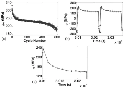
material’s yield surface and, therefore, a progressive variation in the total stress measured in a uniaxial specimen. Typical experimental results for a P19 steel under isothermal (600°C) conditions are presented in Fig. 1. Several different regions of the stress output data may be of interest during an optimisation routine (due to dominant deformation mechanisms

turn can be used to estimate when failure will occur (note the tertiary region in Fig. 1 (a); leading to failure at approximately 600 cycles). General stress magnitudes in loading cycles (see Fig. 1 (b)) are also of interest to determine the specific hardening behaviour for a given cycle. Stress relaxation during strain hold periods (Fig. 1 (c)) is considered due to the creep dominance in this region. Creep is an important factor in high temperature structures and the accurate prediction of this behaviour is of great value to many industries.

Figure 1 - Typical experimental data from dwell type strain controlled test on a P91 steel at 600°C. Figures show (a) the evolution of the stress range (Δσ) over the entire test duration, (b) typical stress versus time loops (at the 150th_/151st _{cycles) and (c) a stress relaxation curve}

observed during a strain hold period (150th cycle).

4.3 Experimental Data Cleaning

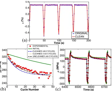
Experimental data will, unavoidably, include scatter. In the domain of cyclic hardening, this may be due to fluctuations in temperature within the test chamber or due to fluctuations in strain rate. Also, inertial effects may cause the test machine to potentially slightly overshoot the maximum or minimum limit strains. Due to the large amounts of data generated, it is of critical importance that as much of the handling process is as automated as possible. Scatter can however result in incorrect points being selected as cycle ends (causing incorrect

Figure 2 – (a) Example of the effect of cleaning on the strain profile (note maximum strain is held over hold period in cleaned data); (b) Fitting of stress range variation (indicating primary

softening behaviour) and (c) Stress values for the final (49th) cycle, by various methods based on an optimisation performed for 49 cycles of P91 data at 600°C.

5

Results for a P91 Steel at 600°C

P91steel experimental data were presented and analysed using the described optimisation procedure. Tests use a “dwell” type strain profile, as described in section 4. Temperature uniformity of the specimen gauge section was such that the entire gauge section was within ±10°C of the testing temperature. Cyclic softening behaviour was observed 9, 20_{. The}

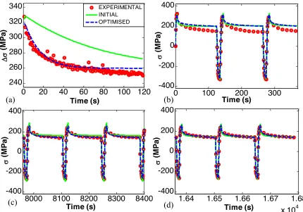
optimisation process was performed based on 120 cycles. A summary of the optimised material constants is given in Table 1 (note the initial estimates are taken from Saad et al 15; derived using the procedure detailed by Tong et al 1 _{and Gong et al} 2_{). Stress range fitting is}

plotted using experimental data, along with initial estimates and optimised values of the Chaboche material constants for predicted behaviour, in Fig. 3 (a). The fitting of the stress versus time profiles for the first, middle and final cycles are displayed in Figs. 3 (b)-(d).

Table 1 - Summary of initial estimates and optimised material constants for the Chaboche model, describing P91 at 600 °C and using 120 cycles of data.

a1 (MPa) C1 a2 (MPa) C2 Z (MPa.s1/n) n b Q (MPa) k (MPa) E (MPa)

Initial 52.20 2060.00 67.30 463.00 1750.00 2.70 1.00 -75.40 85.00 1.39E+05 Optimised 39.99 1284.51 44.28 241.76 476.90 11.16 4.87 -65.84 0.51 1.33E+05

0 10 20 30 40 50 240 260 280 300 320 340 Cycle Number D s ( M P a )

6400 6500 6600 6700 -300 -200 -100 0 100 200 300 Time (s) s ( M P a ) EXPERIMENTAL INITIAL

CLEANED (49 CYCLES) CLEANED (122 CYCLES) UNCLEANED (49 CYCLES)

(a) (b)

0 10 20 30 40 50 240 260 280 300 320 340 Cycle Number D s ( M P a )

6400 6500 6600 6700 -300 -200 -100 0 100 200 300 Time (s) s ( M P a ) EXPERIMENTAL INITIAL

CLEANED (49 CYCLES) CLEANED (122 CYCLES) UNCLEANED (49 CYCLES)

(a) (b)

0 50 100 150 200

Figure 3 – Results of optimisation using 3 objective functions and the Chaboche model for a P91 steel at 600°C (based on 120 cycles of experimental data) showing fitting of (a) stress range, (b) stress values for the first cycles, (c) stress values for the middle (60th) cycles and

(d) stress values for the final cycles.

6

Optimisation from Multiple Experimental Data Sources

In some cases, several different loading wave forms may be applied in isothermal

experimental programs. For example, “saw tooth” type loading profiles (shown in Fig. 4 (a)) will not have a hold period at the end of a tensile loading branch (note this is included in the “dwell” type profile, Fig. 4 (b)). Viscous mechanisms dominate the stress relaxation observed during hold periods (Fig. 4 (d)), therefore it has been suggested that creep or viscous stress material constants may be determined from the stress relaxation periods in dwell type experimental data. Similarly, by using saw tooth type experimental data, the effects of hardening may be isolated and related material constant values estimated. In reality however, controlling deformation mechanism do not act independently (i.e there is some creep

relaxation even during hardening periods). This provides further motivation for optimising material constants in the Chaboche model after an initial estimation procedure.

Experimental data may be generated for one of a multitude of loading waveforms. Constitutive material models such as the Chaboche model should be able to predict the material response for all loading waveforms provided certain loading conditions are satisfied. For example, strain rate or temperature dependencies are not examined in the presented form of the Chaboche model (equations (1)-(4)). Considering two different isothermal loading waveforms performed using the same strain rate and for the same temperature, two different material responses will of course be observed (see Fig. 4 for an example). A single set of Chaboche material constants should however be sufficient to predict both material responses. Several optimisation strategies for producing a single set of material constants from multiple

0 20 40 60 80 100 120

240 260 280 300 320 340 Time (s) D s ( M P a )

0 100 200 300

-400 -200 0 200 400 Time (s) s ( M P a )

8000 8100 8200 8300 8400

-400 -200 0 200 400 Time (s) s ( M P a )

1.64 1.65 1.66 1.67 1.68

x 104

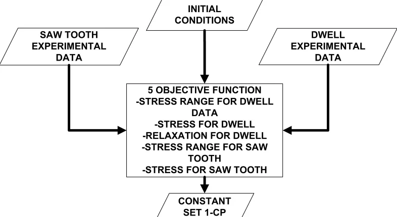
different (but comparable, based on a constitutive model’s dependencies) experimental data sources were proposed and evaluated in a previous publication 21. A “combined parallel” optimisation procedure (whereby objective functions are evaluated simultaneously for each experimental data source, see Fig. 5) was found to be superior due to the maximum amount of optimisation “constraint” being enforced during optimisation iterations. The sum of residuals for several different data sources (for example, the data from the hold periods in dwell type results) are concatenated into a single array and are used to determine subsequent optimisation iterations.

Figure 4 - Example of typical (a) saw tooth strain loading profile, (b) relaxation strain loading profile, (c) stress response due to saw tooth loading profile and (d) stress response due to

relaxation loading profile.

Figure 5 - Flowchart of the combined parallel optimisation procedure. INITIAL

CONDITIONS SAW TOOTH

EXPERIMENTAL DATA

DWELL EXPERIMENTAL

DATA

5 OBJECTIVE FUNCTION -STRESS RANGE FOR DWELL

DATA

-STRESS FOR DWELL -RELAXATION FOR DWELL -STRESS RANGE FOR SAW

TOOTH

-STRESS FOR SAW TOOTH

7

Closing Remarks

The Chaboche model has the ability to accurately predict the initial non-linear response of a material undergoing isothermal cyclic loading. The material constants in the model can be accurately determined through the use of an optimisation procedure, which in turn can be aided and made more robust by subjecting experimental data to a cleaning procedure prior to the application of the optimisation process. Cleaning will involve the removal of scatter in critical regions of the controlling strain profile. With this taken into account, fitting is greatly improved and the optimisation procedure can be automated with far more confidence. Using a method to estimate initial values of the material constants for P91 material data at 600°C (subjected to strain controlled cycling of ±0.5%, with 2 minute hold periods at 0.5%), good estimations of the stress response can be obtained. The coefficient of determination (often signified by r2, defined as the difference in the sum of squares for the mean and regression lines divided by the sum of squares for the mean line 17) provides a metric with which to gauge fitting quality 17 (in this case comparing experimental results to values predicted by the Chaboche model) and was found to increase from 0.9841 based on the fitting for initial estimates of the material constants to 0.9962 for the optimised values. Future work will focus on the further improvement of the fitting, particularly in the prediction of the stress range for materials that do not respond in the same manner as P91, as well as the prediction of the tertiary region leading to failure, generally thought of to be due to the formation of cavitation damage and cracks 9, 20. Alternatives to the optimisation procedure or general methodology used will also be analysed. The effects of variations in the viscous law material constants (Z

and n) will also be investigated; with a view to improving the stress relaxation fitting quality over a wider cycle range.

Acknowledgements

The authors greatly appreciate the support of both E.ON and the EPSRC (case study award number EP/J50211X/1) through funding this work. Thanks are also extended to Mr Tom Bus and Mr Brian Webster for their assistance in the experimental work.

References

1. J. Tong, J. L. Zhan, and B. Vermeulen, Int J Fatigue, 2004, 26(8), 829-837. 2. Y. P. Gong, C. J. Hyde, W. Sun, and T. H. Hyde, P I Mech Eng L-J Mat, 2010,

224(L1), 19-29.

3. C. Maharaj, J. P. Dear, and A. Morris, Strain, 2009, 45(4), 316-331.

4. G. M. Bakic, V. M. S. Zeravcic, M. B. Djukic, S. M. Maksimovic, D. S. Plesinac, and B. M. Rajicic, Therm Sci, 2011, 15(3), 691-704.

5. R. A. Ainsworth and D. G. Hooton, Int J Pres Ves Pip, 2008, 85(3), 175-182. 6. R. A. Ainsworth, Int Mater Rev, 2006, 51(2), 107-126.

7. J. L. Chaboche and G. Rousselier, J Press Vess-T Asme, 1983, 105(2), 153-158. 8. C. J. Hyde, W. Sun, and S. B. Leen, Int J Pres Ves Pip, 2010, 87(6), 365-372. 9. N. E. Dowling: 'Mechanical behavior of materials : engineering methods for

deformation, fracture, and fatigue', xvii, 912 p.; 2007, Upper Saddle River, N.J., Pearson/Prentice Hall.

10. J. L. Chaboche, Int J Plasticity, 1986, 2(2), 149-188. 11. Z. Mroz, J Mech Phys Solids, 1967, 15(3), 163-&.

14. Z. L. Zhan and J. Tong, Mech Mater, 2007, 39(1), 64-72.

15. A. A. Saad, W. Sun, T. H. Hyde, and D. W. J. Tanner, Procedia Engineering, 2011, 10(0), 1103-1108.

16. G. E. Dieter: 'Mechanical metallurgy', xxiii, 751 p.; 1986, New York, McGraw-Hill. 17. S. C. Chapra and R. P. Canale: 'Numerical methods for engineers', xviii, 968 p.; 2010,

Boston, McGraw-Hill Higher Education.

18. P. Venkataraman: 'Applied optimization with MATLAB programming', xvi, 526 p.; 2009, Hoboken, N.J., John Wiley & Sons.

19. Anon: 'Optimisation Toolbox TM 4 User's Guide', T. M. Inc, 2008.

20. R. I. Stephens and H. O. Fuchs: 'Metal fatigue in engineering', xxi, 472 p.; 2001, New York, Wiley.