arXiv:0904.2127v2 [hep-th] 22 Apr 2009
Neil Bevis,1,∗ Edmund J. Copeland,2,† Pierre-Yves Martin,3, 4,‡ Gustavo Niz,2,§ Alkistis Pourtsidou,2,¶ Paul M. Saffin,2,∗∗ and D. A. Steer3,††
1Theoretical Physics, Blackett Laboratory, Imperial College, Prince Consort Road, London, SW7 2BZ, United Kingdom
2School of Physics & Astronomy, University of Nottingham, University Park, Nottingham, NG7 2RD, United Kingdom
3APC, University Paris 7, 10, Rue Alice Domon et L´eonie Duquet, 75205 Paris Cedex 13, France
4Glaizer Group, 32 rue Guy Moquet, 92240 Malakoff, France
(Dated: October 8, 2013)
We study the evolution of non-periodic cosmic string loops containing Y-junctions, such as may form during the evolution of a network of (p, q) cosmic superstrings. We set up and solve the Nambu-Goto equations of motion for a loop with junctions, focusing attention on a specific static and planar initial loop configuration. After a given time, the junctions collide and the Nambu-Goto description breaks down. We also study the same loop configuration in a U(1)×U(1) field theory
model that allows composite vortices with corresponding Y-junctions. We show that the field theory and Nambu-Goto evolution are remarkably similar until the collision time. However, in the field theory evolution a new phenomenon occurs: the composite vortices can unzip, producing in the process new Y-junctions, whose separation may grow significantly, destabilizing the configuration. In particular, an initial loop with two Y-junctions may evolve to a configuration with six Y-junctions (all distant from each other). Setting up this new configuration as an initial condition for Nambu Goto strings, we solve for its evolution and establish conditions under which it is stable to the decay mode seen in the field theory case. Remarkably, the condition closely matches that seen in the field theory simulations, and is expressed in terms of simple parameters of the Nambu-Goto system. This implies that there is an easy way to understand the instability in terms of which region of parameter space leads to stable or unstable unzippings.
I. INTRODUCTION
Cosmic strings have long been known to arise naturally in a wide class of field theories [1, 2, 3, 4], and recent work has indicated that they may also arise in superstring/M-theory [5, 6], for example through models of brane in-flation [7, 8, 9]. Back in the 1980’s fundamental strings and cosmic strings were considered as separate. Obser-vational constraints on the allowed cosmic string tension had to be violated by fundamental strings in order for them to unify the gauge couplings at high energy [10]. Moreover, whereas cosmic strings could be of cosmologi-cal scosmologi-cales, fundamental type I and heterotic strings were known to be unstable and their natural size was of order the Planck scale [10].
Things changed, however, with the second string rev-olution in which the importance of higher dimensional brane solutions was understood, including new types of strings, and it has since been realized that the extra spa-tial dimensions could be large using warped compactifi-cations (for reviews see [11, 12]). As a consequence, it turned out that the effective string tension of the fun-damental strings could be reduced, and depending on
∗Electronic address: [email protected] †Electronic address: [email protected] ‡Electronic address: [email protected] §Electronic address: [email protected] ¶Electronic address: [email protected] ∗∗Electronic address: [email protected] ††Electronic address: [email protected]
the compactification scheme it became possible to have meta-stable fundamental strings of cosmological length [13, 14, 15].
This has opened up the fascinating possibility that this new class of cosmic strings, formed after a period of infla-tion, could provide a unique window on string theory, via measurements of their imprint on the cosmic microwave background radiation [16, 17, 18, 19, 20, 21], their lensing of distant galaxies [22, 23, 24] or through their production of gravitational waves [25, 26, 27] and massive particles [28, 29].
When two cosmic strings intersect, the traditional lore dictates that they intercommute (swap partners), which in the case of a string looping back and intersecting it-self results in the loop being cut off. For traditional field theory strings (essentially Abelian Higgs strings close to the Bogolmonyi limit) this intercommutation oc-curs with effectively unit probability at each intersection [30, 31, 32, 33, 34]. However in the cosmic superstring case the intercommutation probability would be reduced due to the presence of extra dimensions and a small string coupling constant [35, 36, 37, 38].
is how these would affect the properties of the string net-work and what the observational consequences would be? However, this question is not restricted to cosmic su-perstrings. Even the simplest model of gauge strings (the Abelian Higgs model) can provide stable composites if the gauge coupling is set sufficiently high. Indeed, for part of this article we will use the double U(1) model [39] to explore the properties of the Y-junctions that it permits, thereby increasing the applicability of our in-vestigations, although it should be noted that the mass spectrum of the bound states is a specific prediction for cosmic superstrings that is not reproduced by these field theoretic models.
The focus of this article is simple, a detailed compar-ison of the two approaches that have been adopted to describe the dynamics of strings containing Y-junctions. The first, developed by Copeland, Steer and Kibble in [40, 41] (CKS), is based on modifying the Nambu-Goto action to include junctions, and the second is to describe the strings as composite objects in terms of an underly-ing classical field theory that will allow for the formation of junctions [39],[42]-[49]. Such a comparison has a well established history for ordinary cosmic strings, where it has been shown that the Nambu-Goto action for a rela-tivistic 1D string is an excellent approximation to the dy-namics of widely separated gauge cosmic strings as long as the curvature is on scales far greater than the mi-croscopic string width. Once that regime breaks down, the Nambu-Goto approximation is no longer such a good approximation to the full field theory (for a review see [2, 3]). How does the comparison fare for these more complicated arrangements representing strings with junc-tions, and full loop configurations? Recently Bevis and Saffin [49] showed that the results obtained by CKS for the collision of straight strings are consistent with those found using field theory simulations of the double U(1) model, once the composite region grows to be much larger than the string width. This is quite remarkable given the fact that the conditions for Nambu-Goto applicability are breeched in the region of the Y-junction at all times (a related result was also shown for a different field theory model in [50]).
[image:2.612.317.564.50.181.2]In the following, we employ the CKS approach in nu-merical simulations for the first time, exploring scenarios not available through analytical means and in doing so we provide a quite different comparison with field the-ory simulations to that previously performed. Of par-ticular note, we are able to address directly questions such as how closely the two approaches match, where the deviations arise and whether we can safely adopt the Nambu-Goto formalism to describe the evolution of loops containing Y-junctions. The answers to these questions, and in particular the last question is important. It is far easier to evolve a loop based on a modified Nambu-Goto action than on a full field theory action, hence it is possible to analyse a broader class of configurations and obtain more believable statistics concerning the distribu-tion of cusps and kinks on these loops – which in turn
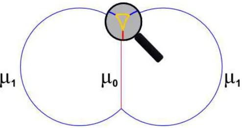
FIG. 1: An example of a loop configuration with multiple junctions: the butterfly configuration with a central string of tensionµ0 and two arc strings of tensionµ1. The basic but-terfly configuration has just two junctions, but we find that under certain situations these can decompose, as indicated by the magnified region, with a single junction splitting into three junctions that then continue to separate.
is important if we want to establish gravitational wave templates for these objects. Motivated by an instability we see in our field theory simulations, we also study it in the context of the Nambu-Goto approach, both analyt-ically and numeranalyt-ically. This then allows us to establish the criteria in terms of a simple angular parameter, un-der which the junctions are stable to unzipping. This in turn will be important in the future when modeling a network of strings with junctions numerically using the Nambu-Goto equations.
For simplicity, and to allow a direct comparison, we concentrate in this paper on a particular type of loop configuration, shown in Fig. 1. It resembles a butterfly and looks somewhat like the result of two co-planar loops colliding. We stress that this is not intended to represent a likely cosmological scenario, but presents an interest-ing case with which we may explore the properties of Y-junctions, including a new feature, their stability to decomposition into three separate Y-junctions.
II. NAMBU-GOTO SIMULATIONS
A. Equations of motion
In this section we set up the Nambu-Goto equations of motion for a string loop withJ junctions, generalising the aforementioned CKS approach that studied the dy-namics of one junction of three strings. For example, a loop with a few junctions is shown in Fig. 1, where the colours differentiate the different charges and tensions of the strings.
1. Case of two junctions
For simplicity, we first derive the equations of motion for a loop with two junctions, which we label by the in-dexJ = (A, B), and three strings. We parameterize the position of theith string (i= 1,2,3) as
xµi(τ, σi), (1)
whereτandσiare the world-sheet coordinates (note that τ is chosen to be the same for all three strings). The induced metric on the world-sheet for stringiis
γi ab=
∂xµi ∂σa
∂xν i
∂σbηµν, (2) wherea= (τ, σi) andηµν is the 4-dimensional Minkowski metric. Below, a dot/dash denotes a derivative with re-spect toτ/σi respectively. The values of the world-sheet coordinateσ at the junction are denoted bysJ
i and are generallyτ-dependent. We are free to choose the direc-tion of increasingσon each string with respect to a given junction. In the case of two junctions, we may takeσto increase from junctionA to junctionB so that
sA
i (τ)≤σi≤sBi (τ). (3) For multiple junctions, as discussed below, this choice cannot always be made. The positions of the junctions are
XJµ(τ) =xµi(τ, sJ
i(τ)) for alli. (4) During the evolution of the loop, it may occur that for one of the strings and at a certain timeτc,sA
i (τc) = sB
i (τc). In that case, the physical length of the string between the junctions vanishes, and the junctions collide. More generally, junctionsAandBcollide whenXAµ(τc) = XBµ(τc) which may occur even if sA
i (τc) 6= sBi (τc) and the length in string i does not vanish. Since in string-theory the outcome of the collision of junctions is not well understood, we will stop our NG simulations of loops at the collision time. The field-theory simulations presented in Sec. III can, of course, go beyond this time.
In the absence of background fluxes and after dilaton stabilisation, the dynamics of asingle infinite(p, q)-string
in flat spacetime is given by the Dirac Born Infeld (DBI) action [51]
SDBI=−µ¯
Z
dτdσp−|γab+λFab|, (5)
where ¯µ = |q|/(gsλ) is the tension of q coincident D-strings, λ = 2πα′, with α′ the Regge-slope parameter, and gs is the perturbative string coupling. Fab is the electromagnetic tensor on the string world-sheet, and the electric flux density is the momentum conjugate to the electric field p = ∂LDBI/∂Fτ σ. The dynamics of three
semi-infinite(p, q)-strings meeting at a junction was
dis-cussed in [51] where it was shown that the resulting equa-tions of motion are exactly equivalent to those obtained by using the Nambu-Goto action for each string,provided
theith string tension in the Nambu-Goto action is taken to be given by
µi =
s
p2 i +
qi
gs
2
, (6)
and one imposes charge conservation at the junction
X
i
pi = 0 X i
qi= 0. (7)
For this reason, and for simplicity, we assume that the dynamics of each individual segment of string is deter-mined by the Nambu-Goto action.
In the conformal gauge
γτ τi +γσiiσi = 0 ; γ
i
τ σi = 0, (8)
the Nambu-Goto action for the three strings of tensions µijoined by two junctions is
S = −X
i µi
Z
dτ
Z
dσi
Θ(sB
i (τ)−σi)Θ(−sAi (τ) +σi)
×q−x′2 i x˙2i
+ X
J=(A,B)
X
i
Z
dτ fJ iµ·[x
µ
i(τ, sJi(τ))−X µ
J(τ)], (9)
whereµiis given in Eq. (6) and the four-vector Lagrange multipliersfJ
iµ(τ) impose the constraints given in Eq. (4). Varying the action (9) with respect to xµi yields the usual equation of motion for a string in Minkowski space-time (away from the junction), namely the wave equation
¨
xµi −xµi′′= 0 =⇒ xµi =1 2[a
µ
i(ui) +b µ
i(vi)], (10) where
ui=σi+τ ; vi=σi−τ. (11) From the conformal gauge conditions (8) the “left” and “right” movers satisfy
Furthermore, varying the action with respect toXJµ, im-posing the temporal gauge and using the boundary condi-tions gives energy conservation equation at each junction (see [40] and appendix A for details):
µ1s˙J1 +µ2s˙J2 +µ3s˙J3 = 0. (13) As the junction is moving, some of the strings will have
˙ sJ
i > 0 while others ˙sJi < 0. These represent grow-ing/shrinking of the string not only in σ-space, but also in real space. The rate of creation of one string must balance the disappearance of other(s).
Given an arbitrary initial loop configuration (xi(0, σi),
˙
xi(0, σi)), we aim to solve the above equations in time in
order to give the full loop evolution and hence (xi(t, σi),
˙
xi(t, σi)). We will now concentrate on junction B. Let
us first define the “communication route” on the loop for a timet at a junctionB by
ℓBmin(t) = min i |s
B
i (t)−sAi(0)|. (14) For a timet < ℓB
minjunctionB receives no influence from the dynamics at junction A, with the initial conditions specifying the incoming waves bµi at B, so determining the behaviour of the junction. For times beyondℓB
min, on the other hand, vertexB is affected by the dynamics at vertexAand the problem becomes more complex. While in Appendix B we shall obtain analytical results that are valid for all times before the two junctions meet, this should be considered a special case and in general nu-merical methods are required.
The general formalism is fully described in appendix A. The amplitudes of the outgoing wavesa′iµ are deter-mined by the amplitudes of the incoming waves b′iµ at the junction, and we find
( ˙sB i + 1)a
′µ i =b
′µ i (1−s˙
B i )−
2
P
kµk
X
j
µj(1−s˙B j)b
′µ j ,
(15) while the evolution of ˙sB
i is determined by
1−s˙B i (t) =
(P
jµj)Mi(1−cBi (t)) µiP
kMk(1−cBk(t))
, (16)
where
cB
1(t) = b′2(v2B(t))·b′3(vB3(t)), (17) M1 = µ21−(µ2−µ3)2, (18) and cyclic permutations. Note that it follows from (16) and imposing causality that one must haveMj ≥0. This is automatically satisfied by (p, q) strings with tensions satisfying Eqs. (6) and (7). At vertexAthe procedure is similar, though the incoming waves are now given by the a′iµ.
2. Multiple junctions
Finally, we now generalize the above formalism to a string loop with more than two junctions. The impor-tant point here is that it is no longer possible to choose theσi’s all to increase (or all to decrease) into a given junction. This can be seen, for example, by considering carefully the triangular section of the loop shown in figure 1. Hence we must treat cases in which there is a different orientation between the three strings at a junction.
To do so we associate a further parameterδJ
i with the 3 strings meeting at junctionJ. IfδJ
i = +1 then on string i, σi increases into the junction. If, on the other hand, δi =−1 for stringi thenσi decreases into the junction. In the action, δJ
i therefore ensures invariance under σ-reparametrisations, and full details are given in appendix A. Note also that the values ofδJ
i for two junctions that are connected by the same piece of string are related. The energy conservation equation at the junction is now generalized (see appendix A) to
δ1Jµ1s˙J1+δJ2µ2s˙J2+δJ3µ3s˙J3 = 0. (19) For example, consider δJ
1 = δ2J = +1 but changing the σorientation of string 3. Then ˙sJ
3 picks up a minus sign but δJ
3 =−1, so the energy equation is unchanged and energy is still conserved. Finally, the formula for the ˙si as a function of the incoming waves at a given junction J is
˙ sJ
i(t) =δi 1− (P
jµj)Mi(1−cJi(t)) µiP
kMk(1−cJk(t))
!
, (20)
where
cJ
i(t) = Yj·Yk, (21) withi6=j6=kand
Yj=
b′
j if δjJ= +1
−a′
j if δjJ=−1.
B. Numerical approach
While the above equations allow for analytical calcula-tions for some particularly simple initial condicalcula-tions (typ-ically semi-infinite straight strings) [40, 41], here we con-sider more complex loop configurations for which numer-ical methods are necessary. We proceed in the following way. For every stringiconnecting two junctions, we work entirely witha′ andb′, reconstructing the closed string
position x(t, σi) and velocity ˙x(t, σi) only when
neces-sary. The initial conditions fix the initial string tensions µi satisfying the triangle inequalitiesMj ≥0, as well as
a′
i(σi) and b′i(σi) between all the junctions. Then we calculate the cJ
i(t = 0) from which ˙sJi(t = 0) is deter-mined using Eq. (20). Then at time δt, sJ
i(δt), uJi(δt) andvJ
(or the appropriate generalized formula in the case of dif-ferent relative orientation of the strings, see for example eq. (A8)) at each junction to extend the domain of defi-nition ofa′
i(u) andb′i(v). The time loop then continues. Our simulation ends whenever the length of one string goes to zero (so whenever two junctions meet). However, the field theory simulations described in the next section can of course continue beyond this time.
C. Initial conditions
We consider belowtwodifferent initial conditions that, as we shall describe, are closely related.
Thefirstis the butterfly configuration shown in Fig. 1,
consisting of only two junctions (in other words, the small triangle shown in the magnifying glass is not present in this initial configuration). More specifically, this planar configuration consists of a straight string with tensionµ0 and two circular arcs with equal tensions µ1. We take the strings to be initially static at all points: at the site of the Y-junctions this requires ˙sj = 0 which is satisfied when the vector sum of tensions at the junction is zero, namely
X
j µj x
′ j
|x′ j|
= 0. (22)
This corresponds, physically, to the fact that there can be no change in momentum occurring within a small vol-ume surrounding the junction if the situation is static, and is in fact the same condition as derived in Appendix A, Eq. (A3) for the case of the static string. This con-dition yields a relationship between the string tensions, the radiusrof the two arcs making the butterfly “wings”, and the distancexof straight string from their centres:
µ0 2µ1
=x
r ≡R. (23)
The second initial condition is a modification of the
[image:5.612.326.562.492.562.2]first initial condition, in that we add, at each junction, the triangular shape shown in the magnifying glass in Fig. 1. Hence this initial configuration consists of 9 strings and 6 junctions, all of which are static. All the strings within the small triangles are taken to be arcs of circles, and are all given the same tension µ2. The rea-son for considering this second initial condition is that our field theory simulations of the simple butterfly con-figuration (with initially only two junctions) will show (see section IV C) that the central straight string can be dynamically unstable into splitting into a configuration very much like the one shown in figure 1. This dynami-cal splitting cannot be accounted for in the Nambu-Goto equations, and hence we are forced to put it in by hand as an initial perturbation. For that reason the initial size
of this perturbation is given by a free parameterh, (effec-tively the distance between one of the old and newly cre-ated junctions), which does not affect the general physi-cal behaviour if initially small; this only depends on the relative tensions of the strings. The fact that the string is initially static sets all angles, shown in Fig. 1, to be functions of the tensionsµi and the parameterh.
Finally, we should note that the use of circular seg-ments to describe the small perturbation is somewhat arbitrary, and it restricts the range of allowed angles (or effectively the value of the tensions µ2 in the perturba-tion) that can be used to construct this second static ini-tial configuration. However, we believe that this choice does not have any dramatic effect on the local dynamics, since it is only the local curvature att= 0 around a given junction that really affects its evolution. We will illus-trate this in section IV C, when studying the stability of Y-junctions.
III. FIELD THEORETIC APPROACH
A. The field theory model
While the Nambu-Goto formalism is relatively easy to analyse numerically, it does not necessarily give a complete description of Y-junctions — for instance, one might expect important interactions between the strings close to and at the junctions, and these are not included in the Nambu-Goto action. For that reason we also study the butterfly configuration, listed above, using a field the-oretic model of gauge strings that permits the formation of junctions.
Strings with junctions can be formed in numerous dif-ferent symmetry breaking schemes: here we study bound states and corresponding Y-junctions of the double U(1) model [39], which has Lagrangian density:
L = −1
4FµνF
µν−(Dµφ)∗(Dµφ)−λ1 4 |φ|
2−η22
−14FµνFµν−(Dµψ)∗(Dµψ)− λ2
4 |ψ| 2
−ν22
+κ|φ|2−η2 |ψ|2
−ν2. (24)
The notation used follows Refs. [39, 49] in that φ and ψare complex scalar fields, each belonging to one of the two Abelian Higgs models that are coupled together via the final term. The gauge-covariant derivatives in the two halves of the model are:
Dµφ = ∂µφ−ieAµφ, (25)
Dµψ = ∂µψ−igBµψ, (26) and the anti-symmetric field strength tensors are:
Fµν = ∂µAν−∂νAµ, (27)
for gauge fieldsAµandBµ. Finally,ηandνare constants that set the energy-scales of the two halves of the model ande.g.λi andκare dimensionless coupling constants.
Forκ= 0 the two halves are uncoupled and the topolo-gies of the vacuum manifolds, each obeying a local U(1) symmetry, require that local string solutions are present [1] (see Refs. [2, 3] for reviews), and take the form of the Nielsen-Olesen vertex [52]. For theφ-half of the model, as a loop enclosing the string is traversed in space, with a net non-zero winding of the phase of φ equal to 2πp (p∈Z), then|φ| is forced to zero along the string in or-der for the field to be smooth. As a result the field does not lie on the vacuum manifold|φ|=ηnear the core and the string carries significant potential energy. It addition-ally carries a quantized amount of pseudo-magnetic flux, equal to 2πp/ein the case of aφstring, since the gauge field acts to reduce the phase gradients and so acquires a significant curl close to the string.
For κ in the range 0 < κ < 12√λ1λ2, two parallel strings from each half can coalesce to reduce the potential energy and hence there are bound string states in this model [39]. Note, however, that for κ > 1
2
√
λ1λ2 the potential term is unbounded from below and the model hence becomes unphysical.
B. Collision of straight strings
The intersection of straight strings has been studied in the above model [49]. It was found that composite states do indeed form and that their growth rates at late times are well predicted by the Nambu-Goto formalism. However, the Nambu-Goto solution differs from the field theory case as the moment of collision approaches, (see also [50] for a similar analysis in the Type I regime of the Abelian Higgs model.) This is partly because any attrac-tion of one string to the other just prior to the intersec-tion event means that the strings are no longer perfectly straight [49]. There are additionally other model depen-dent effects involved in the interaction and it is hence no surprise that the CKS approach differs from the field theory simulation in predicting precisely when the inter-section results in composite formation and growth.
C. Numerical approach
The numerical approach employed for the field theory simulations is largely that of Ref. [49], but with a very dif-ferent set of initial conditions. That is, we use an exten-sion of the Moriarty et al. approach [53] for the Abelian Higgs model with the field evolution then preserving the analogue of Gauss’ law in each half of the model to ma-chine precision. We employ a uniformly-spaced cubic lat-tice, with spacing ∆x, on which the scalar fields are de-fined and then the spatial components of the gauge fields are defined on the links between sites, with the time com-ponents set to zero via a gauge choice. Energy
conser-α=π/2
α=π
[image:6.612.318.561.52.221.2]α=3π/2 α=0
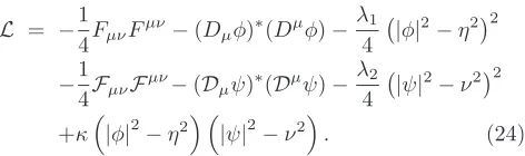
FIG. 2: The initial φ phase choice for a planar (1,0) loop, ensuring a winding of 2πin the desired locations.
vation is accurate so long as the uniform timestep ∆t is sufficiently small.
We obtain the initial conditions required for the but-terfly configuration by first setting up the appropriate windings in the scalar field and then applying a period of dissipative evolution in order to relax the configuration to the minimum energy configuration. That is, during this period there is an extra term in each of the equations of motion that is proportional to the first time derivative of the corresponding field and so removes energy from the system. Additionally we fix the modulus of the scalar field in the region close to the desired centre lines since otherwise the configuration would simply contract to a point during the dissipative evolution. We apply reflec-tive boundary conditions throughout the simulation.
The initial choice for the phases of theφfield for a pla-nar loop of (1,0) string is made as shown in Fig. 2. If a site is above the plane of the loop then it is given the phase π/2, if it is below the plane then it is given 3π/2, while if it is in the plane of the loop then it is given eitherπif it is outside the loop or zero if it is within it. This ensures the correct winding structure of the field but it obvi-ously yields artificially high gradients on the plane of the loop. The modulus of the scalar field is initially chosen so that the field lies on the vacuum manifold, except close to the string centre lines, as will be explained momen-tarily. During the dissipative evolution the gauge field, which is set to zero initially, quickly grows to counter these phases gradients, while the phase and modulus of φrapidly adjust themselves in order to minimize the en-ergy. Obtaining a (0,1) loop can be achieved by simply swapping ψ for φ in the above argument, while a (1,1) loop is yielded by setting up the phases appropriately in both fields. Higher winding numbers cannot be achieved by the direct application of the above approach and will be discussed below.
(2,0)
(1,1) (1,−1)
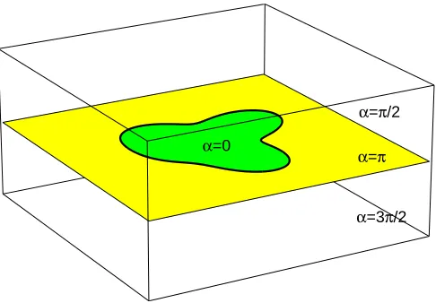
FIG. 3: The fluxes present in the butterfly configuration yielded by the superposition of a (1,1) loop and a (1,-1) loop.
the phase of φ and 2πn in the phase of ψ, this has the following form for small displacements rfrom the string centre:
φ(r)≈Crm, (29) ψ(r)≈Drn. (30) The constants C and D, which are dependent on the choice of m and n cannot be found analytically, but are solved for using essentially the approach of Ref. [39]. Note that ifm is finite but nis zero, then even though there is no winding in ψ, its modulus is still less than ν near the string as this lowers the total potential term energy. However, |ψ| does remain finite as r → 0. In principle we could fix|ψ| close to the string in this case also, but we choose not to since it would not greatly aid the fixing of the string position and we wish to minimize the artificial restrictions enforced.
The butterfly configuration illustrated in Fig. 3 can be constructed by the superposition of a (1,1) loop and a (1,-1) loop after a period of dissipation. Since the equa-tions of motion are non-linear there is no precise means to do this, however a good approximation is simply to sum the gauge fields from each loopA+
µ andA−µ to give the total:
Aµ=A+
µ +A−µ, (31) where the + and−refer to each loop. Then for the scalar fields:
φ η =
φ+ η
φ−
η , (32)
results in a superposition of complex phases [30, 32, 34, 53]. Furthermore, at distances far from any string set up inφ+ (such that the field is approximately constant and close to its vacuum) the form ofφis essentially that found inφ−. Using these equations, the time derivatives must then superpose as:
∂tAµ = ∂tA+µ +∂tA−µ, (33) η ∂tφ = φ+∂tφ−+φ−∂tφ+. (34)
κ 0.80 0.95
µ(1,0)/2πη2 0.864 0.728
µ(1,1)/2πη2 1.452 1.133
µ(2,0)/2πη2 1.622 1.271
R[(1,0) + (0,1)→(1,1)] 0.840 0.778
[image:7.612.56.298.51.192.2]R[(1,1) + (1,−1)→(2,0)] 0.559 0.561
TABLE I: The energy per unit length of an infinite static string, with parametersλ1 = λ2 = 2e2 = 2g2 = 2, η = ν and two values ofκas indicated. Note that an Abelian Higgs string of unit winding would yieldµ= 2πη2[54]. Ris defined in Eq. (23).
While the wings are largely unaffected by this process and remain close to the minimum energy solution, a fur-ther period of dissipation is required to relax the central region, because of the significant interference between the two loops. For the case illustrated in Fig. 3 this includes the cancellation of the fluxes inψalong the central string, which greatly reduces the energy per unit length of that segment.
IV. RESULTS
We shall describe our results in units such that the initial radius of the circular arcs is unity, since this is a useful reference length scale. For the field theory simula-tions we set 2 =λ1=λ2= 2e2= 2g2, since these values are the standard choices [39, 47, 49] and neatly yield the relevant values ofκ in the range 0 < κ <1. We have studied a number of values of κin this range, with 0.8 and 0.95 being the two main ones. We additionally set η=ν and hence there is complete symmetry between the two halves of the model, while we then choose the value of η to set the ratio of the string width (roughly 1/η) relative to the arc radius. Note that although the two Abelian Higgs models are each individually in the Bo-gomolnyi limit [54], with finite coupling between them, theψ field affects the energy per unit length of a (m,0) string even though there is no winding inψ and for ex-ample (2,0) strings are stable (see table I).
In order to compare field theoretic results with those from the Nambu-Goto simulations we additionally cal-culate the string tensions in the case of infinite straight strings via the method of [39]. We then use these asµ0 andµ1 in the Nambu-Goto case, although of course we are also free to choose arbitrary values for these in the Nambu-Goto case. The tensions used are shown in Table I.
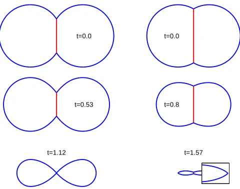
[image:7.612.316.563.53.125.2]t=0.0
t=0.53
t=1.12
t=0.0
t=0.8
[image:8.612.56.296.50.239.2]t=1.57
FIG. 4: Results using the Nambu-Goto method with tensions set to match a field theory (1,0) + (0,1)→(1,1) case with
κ= 0.8 (left plot), and all tensions equal (right plot). The later case corresponds to R = 0.5 and includes a magnified region.
R since most of the energy actually stems from the co-variant derivative term. However a large binding energy can be achieved if the junction involves flux cancellation and therefore we also consider (1,1) + (1,−1) →(2,0). Forκ= 0.95 this yieldsR= 0.56, which indicates that a (2,0) is only slightly heavier than a (1,1) string (which of course has the same tension as a (1,−1) string).
A. Direct comparison of field theory and Nambu-Goto strings.
Before presenting our results it is useful to note that a circular Nambu-Goto loop of unit radius collapses to a point in a timeπ/2. This is also the timescale for collapse of the circular arcs in the butterfly case, though strictly this is limited to regions of the arcs that remain causally disconnected from the junctions during this period (see next section). For the case equivalent to (1,0) + (0,1)→
(1,1) with κ = 0.8, the Nambu-Goto results shown in Fig. 4 (left) reveal that the central bridge string collapses on a timescale shorter than π/2. That is if R = 0.840 the arcs are still largely intact by the time t = 1.12, when the length of the central bridge string is reduced to zero. In contrast for the case corresponding to (1,1) + (1,−1) → (2,0) with κ = 0.95, the more stable bridge remains intact until just prior to the arc collapse: t = 1.56 rather thanπ/2≈1.57. A very similar case to this is shown in Fig. 4 (right), butRhas been set to 0.5 instead of 0.56. This is because we cannot strictly continue the simulation beyond the time of bridge collapse and this choice ofRyields a bridge collapse time that is just longer than the arc collapse time and hence the approximate moment of arc collapse can be seen in the figure.
In Figs. 5 and 6 we compare the field theory results for these two cases with the aforementioned Nambu-Goto ones. The snap shots shown are for equally spaced times and hence additionally show the velocity of the strings. The primary observation is that the agreement between the field theoretic and Nambu-Goto results is excellent for the times shown, allowing us to extend the results from Ref. [49] to strings with global curvature rather than just straight strings with kinks, as was previously consid-ered.
It is also instructive to plot the physical length of the central bridge string as a function of time, as in Fig. 7. For the Nambu-Goto case this can be found analytically via the method of Appendix B and, since this string is stationary, it is just equal to the invariant length:sB−sA. Of course, it can also be obtained from our Nambu-Goto simulations, and provides a nice test of them, however in the field theory simulations, the measurement of the string length is non-trivial.
Fortunately, the geometry of the central bridge is very simple since it merely lies along they-axis at all times. Further we can detect the path of the strings by searching for lattice grid squares around which there is a net wind-ing in the phase of one or both of the scalar fieldsφandψ (using the gauge-invariant method of Ref. [55]). For the case of (1,0)+(0,1)→(1,1) we then search for net wind-ings that lie within a certain threshold of the y-axis and calculate the bridge length as the maximum difference in y-coordinates. There is a small systematic error de-pendent upon the threshold and the angles at which the string arcs meet the bridge string, but this is not relevant. For the second case involving (1,1) + (1,−1)→(2,0), it is useful to note that, as shown earlier in Fig. 3, there is a (0,1) string that passes around the extremes of the con-figuration but not along the bridge. The bridge length can hence be taken to be the distance between the two points where this string meets they-axis.
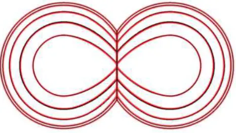
FIG. 5: The evolution of the butterfly configuration (1,0) + (0,1) → (1,1) with κ = 0.8, shown at equally spaced time
intervals: t = 0.000, 0.267, 0.533, 0.800, 1.067, with larger configurations corresponding to earlier times. The field the-ory solution is shown as a bitmap, representing the cumu-lative projection of its energy density onto the plane, while the Nambu-Goto solution is shown as a solid black line. The field theory simulation had lattice spacing ∆x= 0.5/η, with
[image:9.612.61.294.53.185.2]η= 90.
FIG. 6: As in Fig. 5 but forκ= 0.95 and (1,1) + (1,−1)→
(2,0) .
B. Collapse of circular arcs in regions causally disconnected from the junctions
As briefly discussed above, an initially static, circular Nambu-Goto loop of unit radius, collapses to a point in Minkwoski space-time in a time t = π/2. In fact, the Nambu-Goto solution involves the loop radius undergo-ing simple harmonic motion with period 2π. That is, the loop collapses to a point but each segment of the loop re-emerges on the other side of the loop centre. However, the apparent period of the motion is justπbecause seg-ments from one side of the loop are indistinguishable from those on the other side. Not surprisingly, the Nambu-Goto action fails to accurately describe a field theoretic model once the curvature of the string approaches the string width and hence the evolution of the two types of string differs just prior tot=π/2.
0 0.2 0.4 0.6 0.8 1 1.2 1.4 1.6 0
0.2 0.4 0.6 0.8 1 1.2 1.4 1.6 1.8
time
Central bridge length
FIG. 7: The length of the central bridge string as a function of time for the analytic Nambu-Goto solution (thin), the numer-ical Nambu-Goto results (thick, dashed) and the field theo-retic results (crosses). The collection of data with lower bridge lengths is for the (1,0)+(0,1)→(1,1) case withκ= 0.8 while
higher bridge values correspond to (1,1) + (1,−1) →(2,0)
withκ= 0.95. The initial departure of the field theoretic re-sults from the Nambu-Goto ones is due to the measurement technique and is a transient effect.
For the butterfly configuration, by the collapse time, information about the presence of the junction will have travelled around the arcs an angleπ/2, which is just equal to the invariant length traversed for our chosen initial arc radius. Since our initial conditions yield an arc length of 2(π−cos−1(R)) then a length π−2 cos−1(R) remains unaffected by the junctions, which is between 0 and π forRbetween 0 and 1. Hence a fraction of the arcs will collapse to a point, reaching the speed of light for an instant, and yield a sharp kink in the string at a point in physical space. This is confirmed in our numerical simulations and can be seen in the magnified region of Fig. 4. Note that this is not a cusp in the conventional sense, in which the string reaches the speed of light for an infinitesimal range ofσonly. In the butterfly case (with unit initial radius) the change in angle is simply equal to the invariant length involved, and so would be zero for an infinitesimal region.
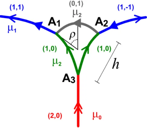
[image:9.612.64.292.314.467.2]ideal-FIG. 8: In the field theory, this diagram shows the possi-ble decomposition of a (1,1) + (1,−1)→(2,0) junction into
three separate Y-junctions. For the Nambu-Goto simulations this can be thought of as the second initial condition (magni-fied region of the butterfly configuration shown in Fig. 1), in which the Y-junction has split into three Y-junctions. In this case, the angles shown would be determined by the tensions,
h, and the fact that the junctions are initially static.
ized initial conditions, we shall not dwell on this region further.
C. Stability of Y-junctions to decomposition into multiple Y-junctions
[image:10.612.55.299.51.264.2]An interesting outcome emerges in the field theoretic case of a (1,1) + (1,−1) → (2,0) junction in that the Y-junction itself can decompose as illustrated in Fig. 8. Whether or not this occurs will depend upon the tensions of the (2,0), (1,1) and (1,0) strings (which cover all ten-sions involved due to the symmetry in our parameter choice) and upon the orientation of the external strings. By coincidenceR=µ0/2µ1is approximately constant for (1,1) + (1,−1)→(2,0) over the range ofκthat we con-sider here (0.8 ≤κ≤0.95). As a resultR is effectively 0.56 over this entire range, essentially fixing both the ini-tial orientations and the large-scale dynamics. However, the ratio ofR=µ1/2µ2(whereµ2is the tension of a (1,0) or (0,1) string) varies from 0.86 to 0.78 asκis increased over that range. Of courseµ0/2µ2must decrease accord-ingly since R is almost constant, and hence both types of composite string become increasingly stable against this decomposition. This can be seen in our results for κ= 0.8, shown in Fig. 9, and those for κ= 0.95 which have already been presented in Fig. 6, where in the new case the junctions decompose and in the previous case they remain stable.
FIG. 9: Results from a field theoretic simulation for (1,1) + (1,−1)→(2,0) withκ= 0.8, showing the decomposition of
the initial Y-junctions. Snapshots are shown for timest= 0, 0.36, 0.8 and 1.24; each representing the cummulative pro-jection of energy density on the plane. The simulation had lattice spacing ∆x= 0.5/η, with η= 90.
The final state of the system is no longer two loops for the cases when the Y-junctions decompose and instead the Y-junctions meet such that the bridge has effectively been cut along its length. There are then two separate loops inφwhich sit at opposite sides of an elongatedψ loop to which they are each bound. These innerφloops then collapse before the outerψloop.
[image:10.612.322.556.59.214.2]accu-rate. However, the approximate matching of the critical value for κ at which the breakup occurs can be consid-ered a considerable success for the less computationally intensive CKS approach, and crucially, as we show be-low, it allows us to make a prediction based purely on the Nambu-Goto results as to when a junction will and will not be stable to decomposition into many junctions. Using the Nambu-Goto approach, the stability of Y-junctions can be studied analytically, at least for small times. In appendix C, we describe this procedure in de-tail for junction A1 in Fig. 8. We find that the initial perturbation in the decomposed state grows or collapses according to the angle ρ (see Fig. 8), which purely de-pends on the original butterfly tensions, the tension of the small arc segments,µ2, and the size of the perturba-tionh, in the following way
ρ= π 2 −cos
−1(
R)−cos−1(R−h), (35) where R= µ1
2µ2 and, as before, R=
µ0
2µ1. Therefore, for
a given pair of tensionsµ0 andµ1 there is a critical ten-sion µ2 = µcrit (for a small fixed h), for which ρ = 0. Below and above this critical limit, there are two distinc-tive behaviours: one in which the perturbation grows (as in Fig. 10) and one in which it either does not grow sig-nificatetly or shrinks, and simply resembles the original butterfly (as in the field theory simulation of Fig. 6). To illustrate this, we can use the analytic results for ˙si and the evolution of the vertexXA1 as a function of the right
(and/or left movers), which explicitly is given by (see Appendix C)
˙
XA1 =− 1
P
jµj
X
j
µj(1−sj)˙ b′
j. (36)
To map the junction movement in real space, it is useful to define the angle
tan(ϕ) = X˙ A1
y ˙ XA1
x
!
, (37)
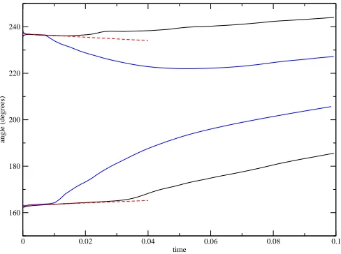
which shows the direction with respect to thex-axis for t > 0. The explicit treatment of this angle is given in appendix C. The main result is that there exists a dis-continuity in ϕ when going from ρ > 0 to ρ < 0, as Fig. 11 shows[56]. This shows how the evolution of the splitting of the Y-junction in the original butterfly de-pends mainly on theinitial local curvature of the strings involved.
When ρ > 0 (see Fig. 8), strings 2 and 3 are “com-peting”in σ-space while the butterfly wing (string 1) is not contributing much (note that for small times ˙s1= 0 to first order in t). After some time and in real space, the vertexA1 moves downwards with an initial angle of ϕ ≥ π+ tan−1(√1−R2/R) (with the equality in the limit ofρ→0) from thex-axis, as can be seen in Fig. 11 (see Appendix C for details of the calculation). In this case the perturbation does not grow and, for a tension
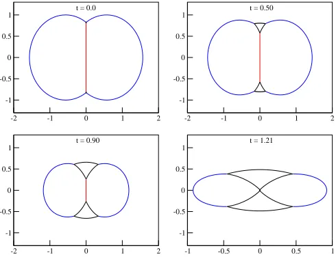
-2 -1 0 1 2
-1 -0.5 0 0.5 1
-2 -1 0 1 2
-1 -0.5 0 0.5 1
-2 -1 0 1 2
-1 -0.5 0 0.5 1
-1 -0.5 0 0.5 1
-1 -0.5 0 0.5 1
t = 0.0 t = 0.50
[image:11.612.318.563.51.239.2]t = 0.90 t = 1.21
FIG. 10: The perturbed butterfly loop corresponding to the
κ= 0.8 field theory case of Fig. 9, using a perturbation param-eterh= 0.01 - the instability grows and the loop is unstable.
µ2big enough, it may even collapse faster than the cen-tral bridge does. However, forρ <0 the local curvature is such that the strings of the triangular perturbation grow inσ-space. In real space, vertexA1initially moves rapidly away from they-axis and almost along the butter-fly wing (string 1), which corresponds to an initial angle ofϕ≤π−tan−1(R/(1−√1−R2) from the x-axis (see Appendix C for details). In figures 10 and 11, one can see this initial evolution. Later in the evolution (when the angleϕreachesπ), the segmentA1A2changes from con-vex to concave, and the vertexA1 evolves like any other point on the big arc segment, hence moving towards the centre of the butterfly wing, as one can see in the last two plots of Fig. 10. Therefore, for ρ < 0 the perturbation grows for some time (which depends on how negativeρ initially is), implying the original butterfly Y-junction is unstable, leading to the criterion for stability based on simply obtaining the value forρ.
V. DISCUSSION
0 0.02 0.04 0.06 0.08 0.1 time
160 180 200 220 240
[image:12.612.55.299.50.232.2]angle (degrees)
FIG. 11: Numerical (solid lines) and analytic (dashed red lines) evolution of the angleϕ, for junction A1, for two cases with ρ > 0 and two with ρ < 0; all close to the critical value ρ= 0 (blue lines are closer to the critical value). For
ρ <0 (bottom curves) the Y-junction is said to be unstable, since vertex A moves along the butterfly wing until it reaches 180◦, and then it starts moving towards the centre of the big arc, as shown in Fig. 10. For ρ > 0 (top curves), vertex A moves downwards, leading to a stable Y-junction. The analytic approximations are calculated usingR= 0.561 and equations (C11) and (C12), which are linear truncations (in time), and only hold for small times since ℓA1min(t) ∼h. We
chooseh= 0.01.
of networks [44, 45, 46, 47], as well as more detailed anal-yses on their individual collisions [49, 50].
The great utility of Nambu-Goto dynamics is the huge reduction in the degrees of freedom compared to field theory simulations, allowing for numerical computations with far larger dynamic range. However, as is well known, the Nambu-Goto dynamics break down as a description of gauged cosmic strings when two vortices cross, loops contract to a point, or when junctions collide. This is well established for the case of the usual Abelian cosmic strings, and algorithms have been developed (motivated by the field theory results) which nevertheless allow the Nambu-Goto equations to be consistently used to model the evolution of a network of cosmic strings (see [3] for details). This same procedure has not yet been estab-lished for the case of strings with junctions, and has been a key goal of this paper. By comparing the modified Nambu-Goto equations for such strings, with the field theory evolution for similar strings we have been able to establish how well they follow each other, and where differences emerge. By concentrating on a simple loop configuration, that nevertheless encapsulates important dynamics, we have been able to explore various prop-erties and directly probe the relationship between these two approaches, answering questions such as: What hap-pens when junctions collide? What is the effect of loop-collapse on the wings of the butterfly loop? What can we say about the instability of junctions as the bound states
try to unzip[48]?
In terms of the general dynamics, we have seen that the evolution of strings with junctions are remarkably well modelled by the Nambu-Goto action [40, 41, 51], despite the curvature at the junctions being high. How-ever, the field theory approach has opened up a crucial new instability that is not present in the usual Nambu Goto formalism, namely the break up of a junction into three new junctions and the corresponding unzipping of the composite string. In other words we still need the field theory to understand the outcome of collisions of strings and collisions of junctions.
Examining the field theory of strings with different binding energies it became clear that for weakly-bound composites the junctions could cause the strings to un-zip, care of the new instability. Once this was realized it became possible to model this within the Nambu-Goto dynamics by introducing the potentially unstable trian-gular configuration at the junctions, and solving for its evolution. Remarkably, this then allowed us to predict in terms of the angleρ(or in terms of the string tensions) when a junction would be unstable to this decay mode, and when it would remain stable, and the results agreed well with the field theory simulations. With this done there is again excellent agreement between the Nambu-Goto simulations and the field theory. The key factor here is that given this understanding of the instability, it is once again possible to perform, with confidence, large-scale cosmological simulations of cosmic superstrings us-ing these modified Nambu-Goto strus-ings, in the same man-ner that it is possible to perform simulations of ordinary cosmic strings using Nambu Goto equations.
VI. ACKNOWLEDGMENTS
We acknowledge financial support from the Royal so-ciety (EJC), STFC (NB and GN) and the University of Nottingham (AP). Field theory simulations were per-formed on the UK National Cosmology Supercomputer (COSMOS) supported by SGI, Intel, HEFCE and STFC. We would also like to thank Tom Kibble for many useful discussions.
APPENDIX A: EQUATIONS OF MOTION
Working in the conformal gauge provides an elegant way to derive the energy conservation equation at each junction. Consider the action given in (9) where we now introduce the parameterδi related to the orientation of the strings at the junction:
S = −X
i µiδi
Z
dτ
Z
dσi
Θ(sBi
i (τ)−σi)Θ(−sA
i
i (τ) +σi)
×
q
−x′2 i x˙2i
+X J
X
i
Z
dτ fJ iµ·[x
µ
i(τ, sJi(τ))−X µ
J(τ)], (A1) whereAi(Bi) is the junction whereσi starts(ends).
Varying the action (A1) with respect toXJµ we have
X
i fJ
iµ= 0. (A2) The boundary conditions, on the other hand, are δiµi(xµi′ + ˙si,Jx˙µi) = fi,Jµ (evaluated at each junction) which, using Eqs. (10) and (A2) gives
0 = X
i µiδi
x′iµ(uJ i) + ˙sJix˙
µ i(viJ)
(A3)
= X
i µiδi
( ˙si+ 1)a′iµ(uJ
i) + (1−si)b˙ ′iµ(viJ)
where uJ
i(τ) =sJi(τ) +τ , viJ(τ) =sJi(τ)−τ. (A4) Note Eq. (A3) reproduces Eq. (22) for the case of a static string ˙si= 0. On imposing the temporal gauge τ =t= x0
i(τ, σi), theµ= 0 component of this equation reduces to energy conservation at each junction:
δ1µ1s˙J1 +δ2µ2s˙J2+δ3µ3s˙J3 = 0. (A5) Now, the constraint that the three strings meet at junc-tionB leads to
2 ˙XBµ = ( ˙sBi + 1)a ′µ i (u
B
i ) + ( ˙si−1)b ′µ i (v
B
i ). (A6) Then we proceed depending on the relative orientation between the 3 strings in question. To illustrate our method, consider the specific example whereδ1=δ2= 1, δ3=−1 for junction B. That is, the incoming waves at junctionB are b′
1, b′2 and a′3. Eliminating the outgoing wavesa′
1,a′2 andb′3 between (A3) and (A6) gives (X
j
µj) ˙XBµ =µ3(1 + ˙sB3)a ′µ 3 −
X
i=1,2
µib′iµ(1−s˙Bi ).(A7)
Eliminating ˙XBµ from Eqs. (A6) and (A7) we can solve for the unknown outgoing waves. This gives
−µ(1 + ˙sB
1)a′1= 2µ2(1−s˙B2)b′2−2µ3(1 + ˙sB3)a′3 +2µ1−
X
j
µj(1−s˙B
1)b′1(A8)
and two similar equations fora′
2 andb′3. Squaring these equations and using the gauge conditions (12) we find eq. (20) withδ1=δ2= 1 andδ3=−1.
APPENDIX B: ANALYTIC RESULT FOR THE BUTTERFLY CONFIGURATION WITH TWO
VERTICES
As discussed in section II A, analytical progress can be readily made for the period before the two junctions
become causally connected. However, since the shortest communication route is the central bridge string, and the symmetry of the butterfly configuration ensures that the only dynamics of the central bridge is for it to change it length, then simple analytical results can be obtained for later times also, as explained below.
The initial conditions are a string lying on they-axis (string 0) and two arcs of unit circles (strings 1 and 2) in the x−y plane. If is useful to introduce an angle γ where, for a static initial configuration, cosγ=−R. We then have:
x0(t= 0, σ0)= (0, σ0,0), |σ0|<sinγ, (B1) x1(t= 0, σ1)= (−cosγ+ cosσ1,sinσ1,0), |σ1|< γ, x2(t= 0, σ2)= (cosγ−cosσ2,sinσ2,0), |σ2|< γ.
If we label the lower vertex as A and the upper one as B, then σi increases towards junction B for all strings. Because of symmetry it is sufficient to study one junction, sayB. Therefore, att= 0
a′0=b′0 = (0,1,0),
a′1=b′1 = (−sinσ1,cosσ1,0),
a′2=b′2 = (sinσ2,cosσ2,0). (B2)
Since the string 0 is simply stationary and on theyaxis for all times, then the abovet= 0 result is valid for allt and the ordinarily difficult to handle emitted waves are simply the waves set by the initial conditions. When the junctions do come into casual contact via string 0, the situation is completely unchanged and hence simple ana-lytical results can still be obtained. Furthermore, string 0 is the shortest communication route, while the results below can be used to show that the two longer routes are always too long to become relevant before the central bridge has collapsed.
Conservation of energy (13) implies that Rs˙B
0 =−s˙B1 and hence after integration we have:
sB
0(t) = sinγ− 1 R s
B 1(t)−γ
. (B3)
Thus, it is sufficient to determine the function sB 1(t). In this case we have c1 = c2 = cos(sB1 −t) and c0 = 2 cos2(sB
1 −t)−1 and so it is useful to denote ∆ =t−sB1, whose derivative is ˙∆ = 1−s˙B
1. Therefore Eq. (16) implies:
˙
∆ = 1−R 2
1 +Rcos ∆. (B4)
This simple separable equation can be integrated to give: tsin2γ=−cosγsin ∆ + ∆−cosγsinγ+γ. (B5) Together with the definition of ∆ and Eq. B3, we now havet, sB
APPENDIX C: STABILITY OFY-JUNCTIONS USING THE NAMBU-GOTO APPROXIMATION
Using the same small time analysis as in Appendix B, we can study the stability of the initial perturbation in-troduced in the butterfly configuration. We will consider junction A1 (see Fig. 8), however this analysis can be equally applied to any other junction. The angles shown in Fig. 8 are completely determined by the initial equi-librium conditions and hence they are defined in terms of the tensions µ1 and µ2. The position of junction A1 inσ-space is
sA1
1 (0) = γ=π−cos−1
µ
0 2µ1−
h
,
sA1
2 (0) = η= cos−1
µ
0 2µ2
−α,
sA1
3 (0) = ρ=γ−α− π
2. (C1)
whereα= cos−1 µ1
2µ2 andhis the distance between
junc-tionA1 (orA2) and junctionA3 in Fig. 8.
We will now analytically demonstrate that the be-haviour of the perturbation (i.e. whether it grows or collapses) depends on whether the angleρis positive or negative. For that we will consider both cases and study the behaviour of ˙sA1
i and X˙A
1. We will drop out the
junction index (A1) from now on for simplicity.
Case I: ρ <0
The initial configuration comprises of three strings with tensionsµ1,µ2 and
b′1(t= 0, σ1) = (sinσ1,cosσ1,0), b′2(t= 0, σ2) = (−sinσ2,cosσ2,0),
b′3(t= 0, σ3) = (−cosσ3,sinσ3,0). (C2)
At a later timetthe incoming waves at junctionAare
b′1(t, s1(t)) = (sin (s1(t)−t),cos (s1(t)−t),0), b′2(t, s2(t)) = (−sin (s2(t)−t),cos (s2(t)−t),0), b′3(t, s3(t)) = (−cos (s3(t)−t),sin (s3(t)−t),0).
(C3) Taylor expandingsi we getsi(t) =si(0) +λit2+... (re-member ˙si = 0 initially), and using the relations between the angles we find (to first order int)
c1 = cos (2α+ 2t), c2 = −cosα,
c3 = −cos (α+ 2t). (C4) Now, using equation (16), linearising in t and defining
R= cosα= µ1
2µ2 (which is always less than unity due to
the triangle inequalities) we find
˙
s1=−s˙3=−√ 1
1− R2t, s˙2=
2R −1 1− R2
t. (C5)
Case II: ρ >0
In this case, the initials conditions can be written as
b′1(t= 0, σ1) = (sinσ1,cosσ1,0), b′2(t= 0, σ2) = (−sinσ2,cosσ2,0),
b′3(t= 0, σ3) = (−cosσ3,−sinσ3,0). (C6)
Following the same procedure we find
˙
s1= 0, s˙2=−s˙3=−2
√
1− R2
1 +R t. (C7)
Having the analytic expressions for ˙si (which of course can be extended further than first order int) we can easily find the analytical expression for ˙Xusing equations (A3)
and (A6), to obtain the expression ˙
X=− 1
P
jµj
X
j
µj(1−sj)˙ b′
j. (C8)
In order to study the motion of the vertex in real space, we define the angle
tan(ϕ) = Xy˙˙ Xx
!
. (C9)
Since the expression for this angle is very complicated, one can take the limit in which the perturbation sizeh tends to zero, and also consider small deviations from theρ = 0 case, either with positive or negativeρ. The critical tensionµ2 which leads to ρ = 0 is obtained by setting (35) to zero and solving forµ2, resulting in
µcrit= µ1
2 cos (cos−1(R−h)−π/2), (C10) Therefore, in the limit h → 0 and µ2 = µcrit equa-tion (C8) reduces to
˙ Xy
˙ Xx =−
R 1 +√1−R2+
−1 + 3R2+√1−R2 R2(1 +√1−R2−2R2√1−R2)t
(C11) forρ <0, and
˙ Xy
˙ Xx =
√
1−R2
R −
2 +R2−2√1−R2
2R4 t (C12)
for ρ > 0. Notice that, as one should expect, in the critical tension limitR drops out from the expressions, and onlyR = µ0
2µ1 appears. For both cases (ρ > 0 and
ρ < 0), ˙Xx is initially positive, so it is the y direction which changes. Forρ >0, the vertex A1 moves with an initial angle of
ϕ=π+ tan−1
√
1−R2 R
!
in the critical limit (µ2 = µcrit), and bigger angles for µ2> µcrit; therefore the perturbation does not grow. In contrast, forρ <0, the vertex A1 moves away from the y-axis, with an initial angle of
ϕ=π−tan−1
R
1 +√1−R2
, (C14)
which is practically along the butterfly wing. In this case, the junctions separate initially from each other and the butterfly configuration is unstable.
[1] T. W. B. Kibble, J. Phys. A9, 1387 (1976).
[2] M. B. Hindmarsh and T. W. B. Kibble, Rept. Prog. Phys. 58, 477 (1995) [arXiv:hep-ph/9411342].
[3] A. Vilenkin and E. P. S Shellard, Cosmic Strings and Other Topological Defects, CUP 1994
[4] R. Jeannerot, J. Rocher and M. Sakellariadou, Phys. Rev. D68, 103514 (2003) [arXiv:hep-ph/0308134].
[5] S. Sarangi and S.-H. H. Tye, Phys. Lett. B 536, 185 (2002), hep-th/0204074.
[6] N. T. Jones, H. Stoica and S.-H. H. Tye, Phys. Lett. B 563, 6 (2003), hep-th/0303269.
[7] G. R. Dvali and S. H. H. Tye, Phys. Lett. B 450, 72 (1999), hep-ph/9812483;
C. P. Burgess, M. Majumdar, D. Nolte, F. Quevedo, G. Rajesh and R. J. Zhang, JHEP 0107, 047 (2001), hep-th/0105204;
G. R. Dvali, Q. Shafi and S. Solganik,
[8] S. Kachru, R. Kallosh, A. Linde, J. M. Maldacena, L. McAllister and S. P. Trivedi, JCAP0310, 013 (2003) [arXiv:hep-th/0308055];
H. Firouzjahi and S. H. H. Tye, Phys. Lett. B584, 147 (2004) [arXiv:hep-th/0312020];
[9] C. P. Burgess, J. M. Cline, H. Stoica and F. Quevedo, JHEP0409, 033 (2004) [arXiv:hep-th/0403119]. [10] E. Witten, Phys. Lett. B153, 243 (1985).
[11] J. Polchinski, “String theory. Vol. 2: Superstring theory and beyond,”Cambridge, UK: Univ. Pr. (1998) 531 p [12] K. Becker, M. Becker and J. H. Schwarz, “String theory
and M-theory: A modern introduction,”Cambridge, UK: Cambridge Univ. Pr. (2007) 739 p
[13] E. J. Copeland, R. C. Myers and J. Polchinski, JHEP 0406, 013 (2004), hep-th/0312067 ;
[14] L. Leblond and S.-H. H. Tye, JHEP 0403, 055 (2004), hep-th/0402072;
[15] G. Dvali and A. Vilenkin, JCAP 0403, 010 (2004) [arXiv:hep-th/0312007].
[16] A. Albrecht, R. A. Battye and J. Robinson, Phys. Rev. Lett.79, 4736 (1997) [arXiv:astro-ph/9707129].
[17] N. Bevis, M. Hindmarsh, M. Kunz and J. Ur-restilla, Phys. Rev. D 75, 065015 (2007) [arXiv:astro-ph/0605018].
[18] C. Contaldi, M. Hindmarsh and J. Magueijo, Phys. Rev. Lett.82, 679 (1999) [arXiv:astro-ph/9808201].
[19] N. Bevis, M. Hindmarsh, M. Kunz and J. Ur-restilla, Phys. Rev. Lett. 100, 021301 (2008) [arXiv:astro-ph/0702223].
[20] A. A. Fraisse, C. Ringeval, D. N. Spergel and F. R. Bouchet, Phys. Rev. D 78, 043535 (2008) [arXiv:0708.1162 [astro-ph]].
[21] L. Pogosian, S. H. Tye, I. Wasserman and M. Wyman, arXiv:0804.0810 [astro-ph].
[22] M. V. Sazhin, M. Capaccioli, G. Longo, M. Paolillo and O. S. Khovanskaya, arXiv:astro-ph/0601494.
[23] B. Shlaer and M. Wyman, Phys. Rev. D 72, 123504 (2005) [arXiv:hep-th/0509177].
[24] K. Kuijken, X. Siemens and T. Vachaspati, arXiv:0707.2971 [astro-ph].
[25] T. Damour and A. Vilenkin, Phys. Rev. Lett.85, 3761 (2000) [arXiv:gr-qc/0004075].
Phys. Rev. D64, 064008 (2001) [arXiv:gr-qc/0104026]. Phys. Rev. D71, 063510 (2005) [arXiv:hep-th/0410222]. [26] X. Siemens, V. Mandic and J. Creighton, Phys. Rev.
Lett.98, 111101 (2007) [arXiv:astro-ph/0610920]. [27] C. J. Hogan, Phys. Rev. D 74, 043526 (2006)
[arXiv:astro-ph/0605567].
M. R. DePies and C. J. Hogan, Phys. Rev. D75, 125006 (2007) [arXiv:astro-ph/0702335].
[28] G. Vincent, N. D. Antunes and M. Hindmarsh, Phys. Rev. Lett.80, 2277 (1998) [arXiv:hep-ph/9708427]. [29] M. Hindmarsh, S. Stuckey and N. Bevis, arXiv:0812.1929
[hep-th].
[30] E. P. S. Shellard, Nucl. Phys. B283, 624 (1987). [31] J. Polchinski, Phys. Lett. B209, 252 (1988).
[32] E. J. Copeland and N. Turok, FERMILAB-PUB-86-127-A (1986).
[33] E. P. S. Shellard and P. J. Ruback, Phys. Lett. B209, 262 (1988).
[34] R. A. Matzner, Computers in Physics, Sep/Oct, 51 (1988).
[35] M. G. Jackson, N. T. Jones and J. Polchinski, JHEP 0510, 013 (2005) [arXiv:hep-th/0405229].
[36] M. G. Jackson, JHEP0709, 035 (2007) [arXiv:0706.1264 [hep-th]].
[37] A. Hanany and K. Hashimoto, JHEP0506, 021 (2005) [arXiv:hep-th/0501031].
[38] A. Avgoustidis and E. P. S. Shellard, Phys. Rev. D73, 041301 (2006) [arXiv:astro-ph/0512582].
[39] P. M. Saffin, JHEP 0509, 011 (2005) [arXiv:hep-th/0506138].
[40] E. J. Copeland, T. W. B. Kibble and D. A. Steer, Phys. Rev. Lett.97, 021602 (2006) [arXiv:hep-th/0601153]. [41] E. J. Copeland, T. W. B. Kibble and D. A. Steer, Phys.
Rev. D75, 065024 (2007) [arXiv:hep-th/0611243]. [42] D. Spergel and U. L. Pen, Astrophys. J.491, L67 (1997)
[arXiv:astro-ph/9611198].
[43] P. McGraw, Phys. Rev. D 57, 3317 (1998) [arXiv:astro-ph/9706182].
[44] E. J. Copeland and P. M. Saffin, JHEP0511, 023 (2005) [arXiv:hep-th/0505110].
[45] M. Hindmarsh and P. M. Saffin, JHEP0608, 066 (2006) [arXiv:hep-th/0605014].
[46] A. Rajantie, M. Sakellariadou and H. Stoica, JCAP 0711, 021 (2007) [arXiv:0706.3662 [hep-th]].
[47] J. Urrestilla and A. Vilenkin, JHEP0802, 037 (2008) [arXiv:0712.1146 [hep-th]].
B332, 297 (1994) [arXiv:hep-ph/9405221].
[49] N. Bevis and P. M. Saffin, Phys. Rev. D 78, 023503 (2008) [arXiv:0804.0200 [hep-th]].
[50] P. Salmi, A. Achucarro, E. J. Copeland, T. W. B. Kibble, R. de Putter and D. A. Steer, Phys. Rev. D77, 041701 (2008) [arXiv:0712.1204 [hep-th]].
[51] E. J. Copeland, H. Firouzjahi, T. W. B. Kibble and D. A. Steer, Phys. Rev. D 77, 063521 (2008) [arXiv:0712.0808 [hep-th]].
[52] H. B. Nielsen and P. Olesen, Nucl. Phys. B61, 45 (1973). [53] K. J. M Moriarty, E. Myers and C. Rebbi, Phys. Lett.
B207, 411 (1988)
[54] E. B. Bogomolny, Sov. J. Nucl. Phys. 24, 449 (1976) [Yad. Fiz.24, 861 (1976)].
[55] K. Kajantie, M. Karjalainen, M. Laine, J. Peisa and A. Rajantie, Phys. Lett. B428, 334 (1998), [arxiv: hep-ph/9803367].