University of Warwick institutional repository: http://go.warwick.ac.uk/wrap
This paper is made available online in accordance with publisher policies. Please scroll down to view the document itself. Please refer to the repository record for this item and our policy information available from the repository home page for further information.
To see the final version of this paper please visit the publisher’s website. Access to the published version may require a subscription.
Author(s): MA Juarez
Article Title: Objective Bayes Estimation and Hypothesis Testing: the reference-intrinsic approach
Year of publication: 2005 Link to published article:
Objective Bayes Estimation and Hypothesis
Testing: the reference-intrinsic approach
Miguel A. Juárez
University of Warwick
Abstract
Conventional frequentist solutions to point estimation and hypothesis testing typically need ad hoc modifications when dealing with non-regular models, and may prove to be misleading. The decision oriented objective Bayesian approach to point estimation using conventional loss functions produces non-invariant solutions, and conventional Bayes factors suffer from Jeffreys-Lindley-Bartlett paradox. In this paper we illustrate how the use of the intrinsic dis-crepancy combined with reference analysis produce solutions to both point estimation and precise hypothesis testing, which are shown to overcome these difficulties. Specifically, we illustrate the methodology with some non-regular examples. The solutions obtained are compared with some previous results.
Keywords: Bayesian reference criterion, intrinsic divergence, intrinsic
estim-ator, logarithmic discrepancy, reference prior.
1 Introduction
Two of the most widely studied problems in statistics textbooks are point
estima-tion and precise hypothesis testing. From a frequentist standpoint, maximum
sharp hypothesis testing. Though it is assumed that asymptotic properties of
max-imum likelihood estimators (MLE) usually hold, –e.g. asymptotic normality– this
is not necessarily the case when the sampling distribution is not regular, and
fre-quently ad-hoc modifications are needed, reducing the generality of the procedure.
Moreover, a number of drawbacks have been exposed about the use ofp-values in
sharp hypothesis testing (see e.g. Edwardset al., 1963; Berger and Selke, 1987; Selke
et al., 2001).
From a decision-theoretic Bayesian standpoint, any of these problems may be
posed as {M,π,`,A}, where M = {p(x | ψ),x ∈ X,ψ∈ Ψ} is the sampling
model for the observable x; π(ψ) is a probability density function (pdf)
describ-ing the decision maker’s prior beliefs about the parameter ψ; A is the space of
possible actions; and`(ψ,a) is a loss function that measures the consequences of
deciding to act according to a ∈ A, when the true value of the parameter is ψ.
Bayes decision rule, that which minimises the posterior expected loss, is then
op-timal for the specific problem at hand. However, in some circumstances such as
scientific communication or public decision making, there is a need for a solution
that lets the data speak for itself or that introduces as little subjective information
as possible. It may also be the case that the decision maker wants to assess the
im-pact that different subjective inputs (both on the prior and the loss functions) have
on the final decision, and thus, a benchmark solution is needed. Objective Bayes
methods are aimed to provide such solutions.
From an objective Bayesian perspective, it is well known that the irrespective
use of “flat” priors may be misleading. Furthermore, Jeffreys’ prior may not be
defined when the assumed model is non-regular. Likewise, though point
estimat-ors derived from “automatic” loss functions –quadratic, zero-one and linear– may
be viewed as acceptable location measures of the quantity of interest, their lack of
invariance under bijective transformations (with exception of the one-dimensional
median) may be suspicious for scientific purposes, where a specific parametrisation
Regarding sharp hypothesis testing, the use of improper priors may lead to
in-determinate answers. The commonly used tool to overcome this problem,
conven-tional Bayes Factors (Jeffreys, 1961, §5.2), assumes that the prior has a point mass
on the null value. This setting leads to what is come to be known as the
Jeffreys-Lindley-Bartlett (JLB) paradox (Bartlett, 1957; Lindley, 1957). Although there has
been some attempts to overcome these disadvantages (Berger and Pericchi, 2001;
O’Hagan, 1995; Robert and Caron, 1996), the resulting factors do not necessarily
correspond to any prior, thus being open to criticism.
This paper illustrates how we can merge the use of the reference algorithm
(Ber-ger and Bernardo, 1992; Bernardo, 1979) to derive non-informative priors, with the
intrinsic discrepancy(Bernardo and Rueda, 2002; Bernardo and Juárez, 2003) as loss
function to obtain an objective answer for both problems. Objective in the precise
sense of only depending on the data and the sampling model. The paper is
organ-ised as follows: in Section 2 the general framework is described, in Section 3 some
non-regular models will be analysed using the proposed methodology and a few
final remarks are presented in Section 4.
2 The Reference-Intrinsic Methodology
Assume it is agreed that the probabilistic behaviour of an observable, x, is well
described by the model M = {p(x | θ,λ), x ∈ X, θ∈ Θ,λ∈ Λ}, and that one
is interested in testing whether the (null) hypothesis H0 ≡ {θ=θ0} is compatible
with the data. Bernardo (1999) argues that this situation may be posed as a decision
problem where the loss function is conveniently described by a proper scoring rule,
derived from the Kullback-Leibler (directed) divergence from the assumed model
to the simplified model induced by the null,M0 = p(x | θ0,λ), i.e.
k(θ0 | θ,λ) = inf λ0∈Λ
ˆ
X
p(x | θ,λ)log p(x | θ,λ)
p(x | θ0,λ0) dx.
statistics starting with the works of Kullback (1968) and Kullback and Leibler (1951).
Robert (1996) regards it as an intrinsic loss in order to address point estimation
within a decision-theoretical framework and Gutiérrez-Peña (1992) derives some
properties when the assumed distribution is a member of the exponential family.
Bernardo (1982, 1985); Bernardo and Bayarri (1985); Ferrándiz (1985) and Rueda
(1992) make use of it in particular hypothesis testing settings.
Noting that the quantity of interest in a decision problem is that which enters
the loss function,k =k(θ0 | θ,λ)is then taken as the quantity of interest for which
the reference posterior,πk(k | x), is derived. Consequently, the posterior expected
value of the logarithmic divergence
d(θ0,x) =
ˆ
kπk(k | x)dk,
gives a measure of the discrepancy from the true, full model to the simplified one,
given by the data.
Recently, Bernardo and Rueda (2002) propose a more general form for the loss
function, namely
Definition 1 (Intrinsic discrepancy).
Assume thatM = {p(x | θ,λ), x∈ X, θ∈ Θ,λ ∈ Λ} is a probability model that
de-scribes the random behaviour of the observable quantity x. The intrinsic discrepancy
(loss)of using the simplified model, with fixedθ=θ0, instead of the full model is given by
δ(θ,λ;θ0) = min
n
k(θ0 | θ,λ),k(θ,λ | θ0)
o
,
where
k(θ0 | θ,λ) = min λ0∈Λ
ˆ
X
f(x | θ,λ) log f(x | θ,λ)
and
k(θ,λ | θ0) = min λ0∈Λ
ˆ
X
f(x | θ0,λ0) log f(x | θ0,λ0)
f(x | θ,λ) dx.
The intrinsic discrepancy has a number of appealing properties: it is
symmet-ric, non-negative and vanishes only if f (x | ω,γ) = f (x | θ,λ) a.e. Is additive
for conditional independent quantities, in the sense that if z = {x1, . . . ,xn} are
independent given the parameters, then δz(θ;θ0) = ∑ni=1δxi(θ;θ0). Is invariant
under one-to-one transformations of both the data and the parameter of interest
and it is also invariant under the choice of the nuisance parameter. Moreover, if
f1(x | ψ)and f2(x | φ)have nested supports so that f1(x | ψ) >0 iff x∈ X1(Ψ),
f2(x | φ) >0 iffx ∈ X2(Φ)and eitherX1(Ψ) ⊂ X2(Φ)orX2(Φ) ⊂ X1(Ψ), the
in-trinsic divergence is still well defined and reduces to the logarithmic discrepancy,
viz. δ(φ;ψ) = k(φ | ψ) when X1(Ψ) ⊂ X2(Φ) and δ(φ;ψ) = k(ψ | φ) when
X2(Φ) ⊂ X1(Ψ) (for a thorough discussion, see Bernardo and Rueda, 2002; Juárez,
2004).
As mentioned above, the posterior expected intrinsic discrepancy, hereafterthe
intrinsic statistic,
d(θ0 | x) =
ˆ
Θ
ˆ
Λ
δ(θ,ω;θ0) πδ(θ,λ | x)dθdλ, (1)
is a measure, in natural information units (nits; bits, if using log2), of the evidence
against using p(x | θ=θ0,λ), provided by the data x. It is a monotonic test
stat-istic for the (null) hypothesis, H0 ≡ {θ=θ0} and thus induces the decision rule,
hereafter the Bayesian reference criterion (BRC):
Reject θ=θ0 iff d(θ0 | x) >d∗.
likeli-hood ratio against using the simplified model, given the data. Hence, values ofd∗
around 2.5 would imply a ratio ofe2.5 ≈ 12, providing mild evidence against the
null; while values around 5 (e5 ≈ 150) can be regarded as strong evidence against
H0; values ofd∗ ≥7.5 (e7.5≈1800) can be safely used to reject the null.
As a natural consequence of the decision-theoretic approach taken here, the best
approximation p(x | θ∗,λ) to the full model p(x | θ,λ), given the data, is given by thatθ∗ which makes the intrinsic discrepancy loss as small as possible. Thus, it is natural to define (Bernardo and Juárez, 2003)
Definition 2 (Intrinsic estimator).
Theintrinsic estimator,θ∗, ofθis the minimizer of the intrinsic statistic, i.e.
θ∗ =θ∗(x) = min θ0∈Θ
d(θ0 | x).
Both the expected intrinsic discrepancy and the intrinsic estimator share a
num-ber of attractive properties (Bernardo and Rueda, 2002; Bernardo and Juárez, 2003):
they are invariant under monotonic transformations ofθandx, and to choice of the
nuisance parameter, are consistent with sufficient statistics, avoid the
marginalisa-tion paradoxes (Dawidet al., 1973) and the expected intrinsic discrepancy avoids
theJLB paradox. Moreover, in contrast with the vast majority of the methods
pro-posed to deal with these problems, its application does not depend on the
asymp-totic behaviour of the model.
3 Examples
In this next section, we will restraint our attention to some simple non-regular
mod-els, applying the methodology described above and then comparing the results
with some of the most common answers in the literature. In order to clarify the
concepts introduced above, we will analyse in first place a one parameter,
3.1 Laplace Model
The Double-Exponential (Laplace) distribution, De(x | 1,θ), with pdf
p(x | θ) = 1 2 exp
h
− |x−θ|
i
, x∈ R, θ ∈R,
does not belong to the exponential family and, thus, does not admit sufficient
stat-istics of fixed dimension. In addition, theMLEis not necessarily unique. In fact, for
m = 1, 2, . . .
ˆ θ =
x((n+1)/2) n =2m
any point ∈ nx(n/2),x(n/2+1)
o
n =2m+1 .
On the other hand, the Kullback-Leibler divergence for one observation from
this model,
k(θ2 | θ1) =
ˆ
exp£−|x−θ1|
¤
logexp
£
−|x−θ1|
¤
exp£−|x−θ2|
¤ dx
=|θ1−θ2|+exp
h
−|θ1−θ2|
i
−1,
turns out to be symmetric, from which
δ(θ;θ0) =|θ−θ0|+e−|θ−θ0|−1 .
The intrinsic discrepancy is a piecewise one-to-one function of the parameter
(Figure 1), permitting the use the reference prior whenθis the parameter of interest
to calculate the intrinsic statistic. It is worth noticing that this model does not meet
the regularity conditions needed to calculate Fisher matrix (see e.g. Schervish, 1995,
p. 111), and thus Jeffreys prior is not defined for it.
By standard properties of reference priors it is easy to prove thatπ(θ) ∝1, and
therefore
π(θ | x)∝exp
"
− n
∑
i=1|xi−θ|
#
-4 -2 0 2 4 -4
-2 0
2 4 0
2 4 6 8
-4 -2 0 2 4 0
2 4 6 8
-4 -2 0 2 4
-4 -2 0 2 4 δ(θ;θ0)
θ θ0
θ
[image:9.595.112.508.77.222.2]θ0
Figure 1.The intrinsic discrepancy (left) and its contour plots for the Laplace model.
Given that the intrinsic discrepancy is a convex function of θ0, the intrinsic
es-timator,
θ∗ =arg min
θ0∈R
ˆ
δ(θ;θ0)π(θ | x)dθ,
is unique (DeGroot and Rao, 1963), and can be readily calculated by numerical
methods. This is illustrated in Figure 2 (a). In this case,x={2.62,−0.08, 1.56,−3.14},
is a simulated sample and the non-uniqueness of the MLE is apparent from the
shape of the likelihood function; however,θ∗ =0.374.
The intrinsic statistic can be calculated by numerical methods and the
approx-imation d(θ0 | x) ≈ δ(θ;ˇ θ0) +1/2, with ˇθ any consistent estimator of θ (Juárez,
2004), works well even for moderated sample sizes, as illustrated in Figure 2 (b).
As stated in the Introduction, from the subjective point of view the Bayes rule
is optimal for the problem at hand. Nonetheless, as the objective solution does not
envisage any specific use, it may be sensible to evaluate the performance of the
intrinsic solutions under repeated, homogenous sampling. To this end we
simu-lated ten thousand data sets for each sample size, with θ = 0. Then the p-value
of the BRC was estimated as the relative number of times that H0 ≡ {θ =0} was
rejected, using the threshold valued∗ =2.5. Regarding the intrinsic estimator, we calculated the relative number of times that it was closer to the true value of the
parameter than theMLE, ˆθ–with the convention that whennis even, theMLEis the
-2 0 2 4 1
2 3 4 5 6 7 8
d(θ0 | x)
l(θ | x)
θ θ∗
(a)Likelihood and intrinsic statistic for simulated sample of sizen=4.
-4 -2 2 4
1 2.5 5 7
d(θ0 | x)
θ0
n=6 n=18 n=3
[image:10.595.102.508.85.254.2](b)Intrisic statistic and the proposed approximation.
Figure 2. Laplace Model. Depicted in the left pane is the (scaled) likelihood and the intrinsic statistic for the simulated sample of size n = 4, also the intrinsic estimator is pointed out. The right pane depicts the intrinsic statistic (solid) and the proposed ap-proximation (dashed) calculated for simulated samples of different sizes andθ = 0. The consistent estimator used for the approximation isθˇ= x.¯
were calculated. The results are summarised in Table 1.
Table 1. Estimatedp-values for theBRCin the Laplace model, using the threshold value
d∗ = 2.5, calculated from 10,000 simulated repetitions for each sample size withθ = 0. Also, the relative number of times (%) that θ∗ was closer thanθˆ to the true value of the parameter, and the mean and (std. dev.) of both estimators for each sample size.
n p-value % θ∗ θˆ
4 0.064 50.4 -2.78×10⁻⁴ (0.633) -1.05×10⁻³ (0.638) 15 0.059 52.9 3.29×10⁻³ (0.299) 2.72×10⁻³ (0.314) 50 0.057 52.5 8.39×10⁻⁴ (0.155) 1.24×10⁻³ (0.159) 100 0.054 52.1 -1.34×10⁻³ (0.106) -8.37×10⁻⁴ (0.108)
The second column exemplifies how the intrinsic statistic is an absolute
meas-ure of the weight of the evidence, brought by the data, against using the simplified
model obtained when lettingθ =θ0. This is in contrast with conventionalp-values
that must be calibrated according to sample size and the dimension of the
para-meter. Summary statistics for both point estimators seem rather similar, suggesting
that sampling properties of the intrinsic estimator are quite in line with those of
[image:10.595.133.476.447.525.2]3.2 Pareto and related models
One of the most appealing characteristics of the reference-intrinsic methodology is
that both the intrinsic statistic and the intrinsic estimator are invariant under
in-vertible transformations, they are also invariant under one-to-one transformations
of the data and under the choice of the nuisance parameter. Here we will illustrate
this point.
There is a vast literature concerning Pareto-like distributions, commencing with
the work of Pareto (1897). It has been used to model a number quantities, including
income, wealth, business size, city size, insurance excess loss, ozone levels in upper
atmosphere (see e.g. Arnold, 1983; Arnold and Press, 1983, 1989). In addition to its
many fields of application, a relevant feature of the classical Pareto pdf,
Pa(x | α,β) = α βαx−(α+1), x ≥β, α,β >0 ,
is its relationship with other widely used models. For instance, letx∼Pa(x | α,β),
then
1.- If y = x−1, then y ∼ Ip¡y | α,βip
¢
, an inverted Pareto distribution; where
βip = β−1and
Ip(y | α,β) = α β−αyα−1, y≤β, α,β>0 .
In particular, Ip(x | 1,β)is a uniform distribution Un(x | 0,β).
2.- If y = −logx, then y ∼ Le(y | α,βle), a location-Exponential distribution;
where βle = − logβand
Le(y | α,β) =α exp
h
−α(y−β)
i
, y ≥β, α>0, β∈ R.
The latter is also a Weibull distribution, Wei(y | 1,α,βle), with
Wei(y | γ,α,β) = γ αγ(y−β)γ−1exp
h
−αγ(y−β)γ
i
which also has a large history of different applications, particularly in
reliabil-ity analysis (see e.g. Nelson, 1982).
In the above distributions, the shape parameter α remains the same, while the
location parameterβi,i = ip,le, is just a one-to-one transformation of the original
location parameter β. Thus, from an objective viewpoint, it seems sensible that
inferences about the parameters conducted with any of the transformed models
should yield the same decisions as those drawn for the original one. This
char-acteristic is apparent for the reference-intrinsic methodology, since for the Pareto
model
δpa(α,β;α0,β0) =
log α α0 +
α0
α −1+α0log β
β0 β≥β0
logα0
α +
α α0 −
1+αlogβ0
β β≤β0
.
On the other hand, for the inverted Pareto model
δip(α,β0;α0,β00) =
log α α0 +
α0
α −1+α0log β00
β0 β0 ≤β00 logα0
α +
α
α0 −1+αlog β0 β00 β
0 ≥β0
0 .
Evidently, if we let β0 = 1/β, both loss functions are identical. For the Weibull model,
δwe(α,β00;α0,β000) =
log α α0 +
α0
α −1+α0(β
00−β00
0) β00 ≥β000 logα0
α +
α α0 −
1+α(β000 −β00) β00 ≤β000 ;
and one can check that when β00 = logβ0 = −logβ, the three functions are the same.
Recall that in this setting, the intrinsic discrepancy is the quantity of interest, and
each of the above loss functions is a one-to-one transformation of any other. Given
that the reference posterior is invariant under these transformations, it follows that
the intrinsic statistic and thereof the intrinsic estimator are also invariant. We can
to the final result. Let us choose the inverted Pareto model.
Suppose we have iid observations,z={x1, . . . ,xn}from an Ip(xi | α,β)
distri-bution, the likelihood function is
L(α,β) =αnβ−nαtnα1 −n; β≥t2,
where {t1,t2} =
n
∏x1/i n,x(n)
o
are jointly sufficient statistics for α and β. The
MLEs
ˆ
β=t2, αˆ =
µ
logt2
t1
¶−1
,
are (conditionally) independent, given the true parameter values (Malik, 1970) and
ˆ
β | α,β∼Ip¡βˆ | nα,β¢ and
ˆ
α | α ∼Ig(αˆ | n,nα),
where Ig(x | a,b)stands for an inverted Gamma distribution with parameters{a,b}.
3.2.1 The shape parameter
In order to apply the definitions in Section 2, we first assume that the shape
para-meterαis the parameter of interest. The intrinsic discrepancy is
δ(α;α0) = n
−logθ+θ−1 θ <1
logθ+θ−1−1 θ ≥1
where θ = α/α0. As δ(θ) does not depend on the nuisance parameter, β, and is
a piecewise one-to-one function ofα, we can derive the reference posterior for the
(marginal) Gamma reference posterior, Ga¡α | n−1,nαˆ−1¢, with pdf
Ga
³
α | n−1,nαˆ−1
´
∝αn−2exp
h −n ˆ α α i .
The intrinsic statistic, forn>2,
d(α0 | αˆ) =
ˆ ∞
0
δ(α;α0)Ga
³
α | n−1,nαˆ−1
´
dα,
can be easily handled by numerical methods. Its typical behaviour, along with the
intrinsic discrepancy, is depicted in Figure 3.
1 2 3 4 1 2 3 4 0 1 2 1 2 3
δ(α;α0)
α α0
(a)Intrinsic discrepancy.
2 4 6 8 10
1 2.5 5 7
d(α0 | αˆ)
α0
n=15
n=3 n=30
n=100
[image:14.595.99.538.306.471.2](b) Intrinsic statistic.
Figure 3. The intrinsic discrepancy –on the left– and the intrinsic statistic calculated for different sample sizes andαˆ =5, in the Inverted Pareto model.
An analytic approximation to the intrinsic statistic (due to the asymptotic
nor-mality of the reference posterior), that works well even for moderated sample sizes
is given by Juárez (2004) as
d(α0 | αˆ)≈δ(α;ˆ α0) + 1 2;
while for the intrinsic estimator we can use
α∗ ≈
µ
1− 3
2n
¶
3.2.2 The location parameter
Consider now the location parameterβ. The intrinsic discrepancy is
δ(β,α;β0) =
log(1−θ) θ <0
θ θ >0
,
whereθ = αlog(β/β0). Recalling the invariance under the choice of the nuisance
parameter, we may use the reference prior for the ordered parametrization{θ,α},
π(θ,α) ∝ α−1, or in terms of the original parametrization,π(β,α) ∝ β−1; yielding the joint reference posterior, forn>2,
π(β,α | t1,t2) = n
n+1
ˆ
αnΓ[n]αnβ−(nα+1)tnα1 ; α >0,β≥t2. The intrinsic statistic,
d(β0 | z) =
ˆ ∞
0
"ˆ
β0
t2
log
µ
1−αlog β β0
¶
π(β,α | z)dβ +
ˆ ∞
β0 µ
αlog β β0
¶
π(β,α | z)dβ
#
dα,
as well as the intrinsic estimator, can be computed numerically. Nevertheless, we
might obtain an analytical approximation by replacingαin the former equation by
itsMLE, ˆαand carrying out the one dimensional integration, obtaining
d(β0 | z) ≈t
h
1+n e−n¡Ei(n)−Ei(n−logt)¢i+n log¡1+ 1 nlogt
¢
,
where Ei(x) = −´−∞xu−1e−udu, andt=¡β/βˆ 0
¢nαˆ
is the usual test statistic arising
from the generalised likelihood ratio. Both the proposed approximation and the
ex-act value of the intrinsic statistic, calculated for some simulated data, are depicted
in Figure 4.
10 20 30 40 50 1
2.5 5 7.5
3.5 4 4.5
1 2.5 5 7.5
d(β0 | z)
n=15 n=30
n=4
d(β0 | z)
n=15
n=4
β0
n=30
β0
[image:16.595.98.505.80.223.2]α<1 α>1
Figure 4. The intrinsic statistic and the proposed approximation (dashed). In the left pane the behaviour forα < 1and in the right pane for α > 1; both are calculated from simulated data of different sizes withβ=3.
is plugging ˆαinto the conditional reference posteriorπ(β | α,z) = Pa(β | nα,t2),
and into the intrinsic divergence and then carry out the one-dimensional
integration-optimisation , resulting in
β∗apr =2n1αˆ β.ˆ
3.2.3 Comparisons
Due to the asymmetry generated by the shape parameter, it seems reasonable that,
for the same sample size, we should have less precise estimates of βwhen α < 1
than when α > 1. Table 2 presents the results obtained from simulated data for a
small sample size and two values for the shape parameter. The behaviour of the
in-trinsic estimator seems to capture the increased variability brought by the different
values of shape parameter better than the MLE. Also, the estimated
p-value for theBRCusing the threshold valued∗ =2.5 is presented.
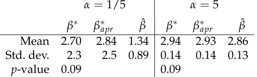
Table 2. Mean value and standard deviation of the intrinsic estimator, the proposed ap-proximation and the maximum likelihood estimator of the location parameter of the Inver-ted Pareto model, calculaInver-ted from 5000 simulaInver-ted samples holdingβ=3and n=4.
α =1/5 α =5
β∗ β∗apr βˆ β∗ β∗apr βˆ Mean 2.70 2.84 1.34 2.94 2.93 2.86 Std. dev. 2.3 2.5 0.89 0.14 0.14 0.13
[image:16.595.176.439.668.747.2]For the sake of comparison, assume now that the shape parameter is known
and, without loss of generality,α =1. It is readily seen that thenx ∼Un(x | 0,β)
and, therefore, −logx = y ∼ Le(y | 1,β0). Each of the correspondent intrinsic discrepancies,
δx(β;β0) =
¯ ¯ ¯ ¯log ββ
0
¯ ¯ ¯ ¯
and
δy(β0;β00) =
¯
¯β0−β0
0
¯ ¯,
is a piecewise one-to-one function of the implied parameter. Thus, we can use
π(β) ∝ β−1and π(β0) ∝ 1, to derive the appropriate reference posteriors, which
are Pa(β | n,t) and Le(β0 | n,t0), respectively, where t = max{x1, . . . ,xn} and t0 =−logt=min{y1, . . . ,yn}.
The calculation of the intrinsic statistics is straightforward,
d(β0 | t) =
ˆ ∞
t
¯ ¯ ¯ ¯log ββ
0
¯ ¯ ¯
¯ Pa(β | n,t) dβ
=2τ−logτ−1
and
d(β0 | t0) =
ˆ t0
−∞
¯
¯β0−β0
0
¯
¯ Le¡β0 | n,t0¢ dβ0
=2τ0−logτ0−1 ,
whereτ = τ(β0,t) = (t/β0)n andτ0 =τ(β0,t) = exp[n(β00−t0)]are the test stat-istics derived from the generalised likelihood ratio. The invariance of the intrinsic
statistic is apparent, it is straightforward to verify thatd(β00 | t0) =d(−logβ0,−logt). Consequently, the intrinsic estimator is also invariant, thus we have β∗(t) = 21/nt
andβ0∗(t0) = −logβ∗ =t0−log 21/n.
Interestingly, under homogeneous repeated sampling, both τ and τ0 follow a Un(y | 0, 1) distribution under the null H0 ≡ {β =θ0(β0 =β00)}. Similarly, from the Bayesian viewpoint,τB = (t/θ)n andτB0 =exp[n(β0−t0)]follow the same
and the Bayesian Reference Criterion, exhibited in Table 3.
Table 3. Some p-values, P[d > d? | H0], associated to the corresponding threshold
values, d∗, from theBRCfor the Uniform model.
d? P[d>d? | H0] d? P[d>d? | H0]
1 0.203 5 0.00278
2 0.054 6 0.00097
2.5 0.031 7 0.00038
3 0.019 8 0.00018
4 0.007 9 0.00008
The risk functionRβ(c)in the Uniform model, for estimators of the form ˜θ =c t,
withc >1, under the intrinsic discrepancy loss function is
Rθ(c) =
ˆ θ
0
n
¯ ¯ ¯ ¯logc tθ
¯ ¯ ¯
¯ nθ−ntn−1dt
=2c−n+nlogc−1.
Straightforward calculations show thatRθ(c)attains a global minimum atc =21/n,
i.e. the intrinsic estimator is the only admissible estimator under the intrinsic
dis-crepancy loss. This same holds forβ0∗in the location-Exponential model for estim-ators within the classC =©β˜ : ˜β=t+c,c <0ª.
The Location-Exponential model is used by Berger and Pericchi (2001) to
illus-trate the use of the intrinsic Bayes factors (IBF) for non-regular cases. There, the
authors compute the arithmetic and the median intrinsic Bayes factors (AIBF and
MIBF, respectively) as
AIBF = B1
n n
∑
i=1£
exp(yi−β00)−1
¤−1
and
MIBF= B £exp(Med[y]−β00)−1¤−1 ,
factor (O’Hagan, 1997),
FBF = B b n ©exp£b n(t0−β00)¤−1ª−1, is clearly unreasonable, given thatFBF >1 for any 0<b <1.
Even though both IBF’s are defined in this case, their behaviour under
homo-geneous repeated sampling is awkward. To illustrate this we simulated 100,000
sets of different sizes from Le(x | 1,−0.1)and then computed the relative number
of times that the (null) hypothesis H0 ≡ {β=−0.1} was rejected. As we can see
from Table 4,p-values arising from alternativeIBF s vary widely with sample size,
[image:19.595.210.403.394.483.2]while those computed from theBRCand the frequentist test behave as expected.
Table 4.Estimatedp-values corresponding to comparable test sizes for theBRC(d∗ =3),
the frequentist test (α = 0.05) and theIBF’s (B ≥ 20) calculated from simulated values
(100,000 replications) from the Location-Exponential model for several sample sizes and
β=−0.1
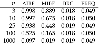
n AIBF MIBF BRC FREQ 3 0.998 0.889 0.018 0.049 10 0.997 0.675 0.018 0.050 25 0.938 0.448 0.019 0.049 100 0.525 0.165 0.018 0.050 1000 0.097 0.019 0.019 0.049
Another anomaly is that it is possible to reach conflicting decisions from
altern-ative IBF for small samples. For instance, consider the simulated data set from a
Un(xi | 0, 1), x = {0.01, 0.05, 0.50, 0.99}, and the transformed data when making
y = −logx. Table 5 shows the alternative Bayes factors and the intrinsic statistic
calculated for testing the (null) hypothesis H0 ≡ {β=1(β0 =0)}. Given the in-variance properties of the intrinsic statistic, clearly d(1 | t) = d(0 | t0) and thus decisions derived from both data sets are the same, for they convey exactly the
same amount of information about the parameter. In contrast, different decisions
Table 5. Alternative intrinsic Bayes factors and the intrinsic statistic to test the hypo-thesis β = 1(β0 = 0), calculated for the simulated data, from a Un(x | 0,β), x =
{0.01, 0.05, 0.5, 0.99}and for the transformed data y=−logx, whereβ0 = −logβ.
AIBF01 MIBF01 d β 5.05 13.97 0.98 β0 3.89 519.21 0.98 3.2.4 USA metropolitan areas
As mentioned at the beginning of the section, Pareto distributions are often used to
model city population sizes. Zipf (1949) formally established that, within a given
country, the size of the k largest cities is inversely proportional to its rank; this
regularity implies that the distribution of the population size of these cities, s, is
Pa(s | α,β), with shape parameter equal to one. To verify Zipf’s law, we
ana-lyse the 276 USA metropolitan areas (MA) population, based on the 2000 census
(www.census.gov/main/www/cen2000.html). Three nested data sets were
con-sidered: data set D1 contains the 50 largest MA’s; data set D2 contains the 135
largest MA’s; and data setD3is the whole sample. The intrinsic estimators for each
case are α∗1 = 1.2, α∗2 = 0.914 and α∗3 = 0.562; intrinsic statistics for each data set are depicted in Figure 5. From these we can state that Zipf’s law holds for the first
two data sets, sinced(1 | D1) = 0.88 andd(1 | D2) = 1.26; whiled(1 | D3) =39.15,
providing overwhelming evidence againstα =1, for the whole of USA MA’s (for a
thorough discussion on this phenomenon see Eeckhout, 2004).
0.5 1 1.5 2
1 2.5 5 7.5
d(α0 | D2)
α0
d(α0 | D1)
(a)The 50 and the 135 largest USA MA’s
0 0.2 0.4 0.6 0.8 1
1 2.5 5 7.5
d(α0 | D3)
α0
[image:20.595.77.524.574.744.2](b) All USA MA’s
3.3 The change-point problem
The change-point problem has an log history, dating back to Page (1955, 1957), and
has been addressed in different ways by Carlinet al. (1992); Hinkley (1970); Smith
(1975), i.a. In general, the problem is to be able to discriminate in a sequence of
independent observations,x={x1, . . . ,xn}, if all members are drawn from a
com-mon distribution,p(x), or if there exists a point,r, for which the firstrobservations
come fromp1(x)and the rest fromp2(x).
This problem may be addressed in two alternative ways:
Retrospective Consider the sequence of observations, x = {x1, . . . ,xn}, as a
real-isation of a concrete process. Determine if there exists a change point, 1≤r<
n(see, e.g. Chernoff and Zacks, 1964; Beibel, 1996 and references therein). Or
Sequential Consider the sequence x = {x1,x2, . . . ,xr,xr+1, . . .}. Determine, as
soon as possible, if a change has occurred at pointr(see, e.g. Shiryayev, 1963;
Lorden, 1971 and references therein).
3.3.1 Page’s artificial data
Here we focus on the retrospective approach and analyse the artificial data of Page
(1957). Thus, we will assume thatp1(x) =N(x | 5, 1)and p2(x) =N(x | 6, 1), so
the likelihood function is
L(θ1,θ2) =
r
∏
i=1N(x | 5, 1) n
∏
j=r+1N(x | 6, 1) 1≤r<n
n
∏
i=1N(x | 5, 1) r=n
. (2)
For this simple setting, the intrinsic discrepancy is the linear loss function,
δ(r;r0) = 1
2|r−r0|.
Hence, the intrinsic estimator is just the posterior median. Asδ(r;r0)is a piecewise
the appropriate posterior, which is proportional to the likelihood.
If both means are unknown, i.e. p1(x) = N(x | µ, 1) and p2(x) = N(x | η, 1),
we get
δ(r,µ,η;r0) = 12(µ−η)2|r−r0|
r
r0 r≤r0
n−r
n−r0 r≥r0 ,
from where it is possible to derive the appropriate reference posterior and then
cal-culate the intrinsic statistic and estimator. Figure 6 depicts the intrinsic statistic for
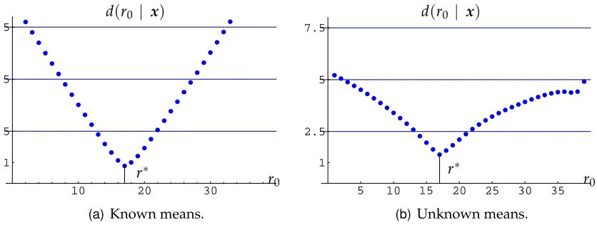
both scenarios. We can see thatr∗ =17, irrespective of the known means assump-tion, coinciding with Page’s analysis. If the means are known, we could say that the
change took place within the 13th and the 21st observations, and we could be quite
sure that no change took place outside the 7th and 27th observations. On the other
hand, if the means are unknown, we could say that a change occurred between
the 15th and 21st observations and were almost sure that no change took place
be-fore the second one. In any case, the true change point, at the 21st observation, is
effectively detected.
10 20 30
1 2.5 5 7.5
d(r0 | x)
r0
r∗
(a) Known means.
5 10 15 20 25 30 35
1 2.5 5 7.5
d(r0 | x)
r0
r∗
[image:22.595.93.511.457.615.2](b)Unknown means.
Figure 6.The intrinsic statistic for the change-point problem, calculated for Page’s data.
3.3.2 River Nile data
Consider the measurements of the annual volume of discharge from the Nile River
to Aswan from 1871–1970, first analysed by Cobb (1978) and further examined from
that p1(x) = N(x | µ,λ) and that p2(x) = N(x | η,λ), with a common unknown
precision,λ, the intrinsic discrepancy and a corresponding reference prior are
δ(r,θ;r0) = n 2 log h
1+r(r0−r) r r0 θ
2i r ≤r
0
log
h
1+(n−r)(r−r0) n(n−r0) θ
2i r ≥r 0
and
π(r,θ) ∝λ−1
³
1+r(n−r) 2n2 θ
2´−1/2,
respectively, where θ = λ1/2(µ−η) is the standardised distance between the two
means.
In this case,r∗=1898, which coincides with the three analyses mentioned above. In addition, the intrinsic change-point regions corresponding to the proposed
thre-shold values are R2.5 = {1897, 1899}, R5 = {1895, 1900} and R7.5 = {1894, 1903}.
If we carry the analysis one step further, and perform inference on the difference of
means,∆ =µ−η, conditional onr=1898, the intrinsic estimator of the change in
the mean (which is also the MLE, see Juárez, 2004) is ∆∗ = 247.78 and the corres-ponding non-rejection regions are R2.5 = {189.69, 305.87}, R5 = {159.65, 335.91}
andR7.5 = {136.50, 359.05}. These results are summarised in Figure 7.
1889 1892 1895 1898 1901 1904 1907 1
2.5 5 7.5
d(r0 | x)
r0
r∗
(a) Change-point.
100 200 300 400 500
1 2.5 5 7.5
d(∆0 | x)
∆0 ∆∗
[image:23.595.82.516.523.680.2](b)Difference in means.
Figure 7. River Nile data. In the left pane, the intrinsic statistic for the change-point. The right pane depicts the intrinsic statistic for the difference in means, conditional on r =r∗ =1898.
prob-lems. The IBF requires a training sample to convert the initial improper prior into
a proper one. However, no minimal training sample exists for the (retrospective)
change-point problem, thus an ad-hoc modification is in needed (Moreno et al.,
2003). In contrast, the reference-intrinsic methodology needs no modification and
renders sensible results.
4 Conclusions
The reference-intrinsic methodology provides objective Bayesian decision rules for
the precise hypothesis testing and point estimation problems, objective in the
pre-cise sense of depending on the data and the sampling model alone. In addition to
this, the point stressed in this paper is that the presented method needs no
modi-fication, regardless the regularity conditions of the sampling model and the
dimen-sion of the parameter.
When testing sharp hypotheses, the use of conventional Bayes factors relies on a
particular prior with a point mass on the null, leading to the so calledJLBparadox.
Alternative Bayes factors are still open to criticism. We have seen how fractional
Bayes factors fail when dealing with non-regular models and it can be shown that
other problems arise in the presence of nuisance parameters. As for intrinsic Bayes
factors, it may be the case (as theAIBF in the exponential location model) that the
resulting factor comes from no prior, thus being not really Bayesian; or that one of
the Bayes Factors (theMIBF in that same example) be biased in favor of one of the
hypothesis. Moreover, it may also happen (like the AIBF) that the resulting Bayes
Factor depends on the whole sample, even when sufficient statistics are available,
thus violating the sufficiency principle. We have also seen that the intrinsic statistic
is typically a one-to-one function of the test statistic derived from the generalised
likelihood ratio, providing a link between the frequentist test and theBRC; indeed,
when this is the case, theBRCmay be seen as a way to calibrate thep-values.
One of the most compelling features of the intrinsic estimator, shared by the
of the parametric space is greater than one, a characteristic not shared by the most
frequently used objective Bayesian point estimators. Additionally, as illustrated
in the examples, it is a consistent estimator of the parameter and, hence, agrees
asymptotically with theMLE–when this exists–, accounting for the increase in
un-certainty when nuisance parameters are present in the sampling model, while
typ-ically exhibiting compelling properties under repeated, homogeneous sampling.
¶ v 1 0
References
Arnold, B. C. (1983),Pareto Distributions, USA: International Co-operative
Publish-ing House.
Arnold, B. C. and Press, S. J. (1983), Bayesian inference for Pareto populations,
Journal of Econometrics,21, 287–306.
Arnold, B. C. and Press, S. J. (1989), Bayesian estimation and prediction for Pareto
data,J. Amer. Statist. Assoc.,84, 1079–1084.
Bartlett, M. S. (1957), Comment on “A statistical paradox” by D. V. Lindley,
Biomet-rika,44, 533–534.
Beibel, M. (1996), A note on Ritosv’s Bayes approach to the minimax property of
the cusum procedure,The Annals of Statistics,24, 1804–1812.
Berger, J. O. and Bernardo, J. M. (1992), On the development of reference priors,
Bayesian Statistics 4(J. M. Bernardo, J. O. Berger, A. P. Dawid and A. F. M. Smith,
eds.), Oxford: University Press, pp. 35–60.
Berger, J. O. and Pericchi, L. R. (2001), Objective Bayesian methods for model
selection: Introduction and comparison, Model Selection, Lecture Notes, vol. 38
(P. Lahiri, ed.), Institute of Mathematical Statistics, pp. 135–207, (with
Berger, J. O. and Selke, T. (1987), Testing a point null hypothesis: The
irreconcilab-ility of p-values and evidence, J. Amer. Statist. Assoc., 82, 112–139, (with
discus-sion).
Bernardo, J. M. (1979), Reference posterior distributions for Bayesian inference,J.
Roy. Statist. Soc. B,41, 113–147.
Bernardo, J. M. (1982), Contraste de modelos probabilísticos desde una perspectiva
bayesiana,Trabajos de Estadística,33, 16–30.
Bernardo, J. M. (1985), Análisis bayesiano de los contrastes de hipótesis
paramétri-cos,Trabajos de Estadística,36, 45–54.
Bernardo, J. M. (1999), Nested hypothesis testing: The Bayesian Reference
Cri-terion,Bayesian Statistics 6(J. M. Bernardo, J. O. Berger, A. P. Dawid and A. F. M.
Smith, eds.), Oxford: University Press, pp. 101–130.
Bernardo, J. M. and Bayarri, M. J. (1985), Bayesian model criticism, Model Choice
(J. P. Florens, M. Mouchart, J. P. Raoult and L. Simar, eds.), Bruxelles: Pub. Fac.
Univ. Saint Louis, pp. 43–59.
Bernardo, J. M. and Juárez, M. A. (2003), Intrinsic estimation, Bayesian Statistics 7
(J. M. Bernardo, M. J. Bayarri, J. O. Berger, A. P. Dawid, D. Heckerman, A. F. M.
Smith and M. West, eds.), Oxford: University Press, pp. 465–475.
Bernardo, J. M. and Rueda, R. (2002), Bayesian hypothesis testing: A reference
ap-proach,International Statistical Review,70, 351–372.
Carlin, B. P., Gelfand, A. E. and Smith, A. F. M. (1992), Hierarchical Bayesian
ana-lysis of changepoint problems,Appl. Statist.,41, 389–405.
Carlstein, E. (1988), Nonparametric change-point estimation, The Annals of
Statist-ics,16, 188–197.
Chernoff, H. and Zacks, S. (1964), Estimating the current mean of a Normal
Cobb, G. W. (1978), The problem of the Nile: Conditional solution to a changepoint
problem,Biometrika,65, 243–251.
Dawid, A. P., Stone, M. and Zidek, J. V. (1973), Marginalization paradoxes in
Bayesian and structural inference, J. Roy. Statist. Soc. B, 35, 189–223, (with
dis-cussion).
DeGroot, M. H. and Rao, M. M. (1963), Bayes estimation with convex loss,The ann.
of Math. Stat.,34, 839–846.
Dümbgen, L. (1991), The asymptotic behavior of some nonparametric change-point
estimators,The Annals of Statistics,19, 1471–1495.
Edwards, W., Lindman, H. and Savage, L. J. (1963), Bayesian statistical inference
for psychological research,Psychological Review,70, 193–242.
Eeckhout, J. (2004), Gibrat’s law for (all) cities,American Economic Review,94, 1429–
1451.
Ferrándiz, J. R. (1985), Bayesian inference on Mahalanobis distance: an alternative
approach to Bayesian model testing,Bayesian Statistics 2(J. M. Bernardo, M. H. D.
Groot, D. V. Lindley and A. F. M. Smith, eds.), Amsterdam: North-Holland, pp.
645–654.
Gutiérrez-Peña, E. (1992), Expected logarithmic divergence for exponential
famil-ies, Bayesian Statistics 4 (J. M. Bernardo, J. O. Berger, A. P. Dawid and A. F. M.
Smith, eds.), Oxford university press, pp. 669–674.
Hinkley, D. V. (1970), Inference about the change-point in a sequence of random
variables,Biometrika,57, 1–17.
Jeffreys, H. (1961),Theory of Probability, 3rd ed., Oxford: University Press.
Juárez, M. A. (2004), Objective Bayesian methods for estimation and hypothesis testing,
Kullback, S. (1968),Information Theory and Statistics, New York: Dover.
Kullback, S. and Leibler, R. A. (1951), On information and sufficiency, Ann. Math.
Stat.,22, 79–86.
Lindley, D. V. (1957), A statistical paradox,Biometrika,44, 187–192.
Lorden, G. (1971), Procedures for reacting to a change in distribution, Ann. Math.
Statis.,42, 1897–1908.
Malik, H. J. (1970), Estimation of the parameters of the Pareto distribution,Metrika,
15, 126–132.
Moreno, E., Casella, G. and García-Ferrer, A. (2003), ObjectiveBayesian analysis of
the changepoint problem,Working Paper 06-03, Universidad Autónoma de
Mad-rid.
Nelson, W. (1982),Applied life data analysis, New York: Wiley.
O’Hagan, A. (1995), Fractional Bayes Factors for model comparison,J. Roy. Statist.
Soc. B,57, 99–138.
O’Hagan, A. (1997), Properties of intrinsic and fractional Bayes factors,Test,6, 101–
118.
Page, E. S. (1955), A test for a change in a parameter occurring at an unknown point,
Biometrika,42, 523–527.
Page, E. S. (1957), On problems in which a change in a parameter occurs at an
unknown point,Biometrika,44, 248–252.
Pareto, V. (1897),Cours d’economie Politique, II, Lausanne: F. Rouge.
Robert, C. P. (1996), Intrinsic losses,Theory and Decisions,40, 191–214.
Robert, C. P. and Caron, N. (1996), Noninformative Bayesian testing and neutral
Rueda, R. (1992), A Bayesian alternative to parametric hypothesis testing, Test, 1,
61–67.
Schervish, M. J. (1995),Theory of Statistics, New York: Springer.
Selke, T., Bayarri, M. J. and Berger, J. O. (2001), Calibration of p-values for testing
precise null hypotheses,The American Statistician,55, 62–71.
Shiryayev, A. N. (1963), On optimum methods in quickest detection problems,
The-ory Probab. Appl.,8, 22–46.
Smith, A. F. M. (1975), A Bayesian approach to inference about a change-point in a
sequence of random variables,Biometrika,62, 407–416.
Zipf, G. K. (1949), Human behavior and the principle of least effort, Cambridge, MA:


![Table 3. Some p-values, P[ d >d|⋆ H]0 , associated to the corresponding thresholdvalues, d∗, from the BRC for the Uniform model.](https://thumb-us.123doks.com/thumbv2/123dok_us/9780735.479173/18.595.191.423.134.230/table-values-associated-corresponding-thresholdvalues-brc-uniform-model.webp)