https://doi.org/10.5194/hess-23-5069-2019 © Author(s) 2019. This work is distributed under the Creative Commons Attribution 4.0 License.
Pattern and structure of microtopography implies
autogenic origins in forested wetlands
Jacob S. Diamond1,2, Daniel L. McLaughlin3, Robert A. Slesak4, and Atticus Stovall5
1Quantitative Ecohydrology Laboratory, RiverLy, Irstea, Lyon, 69100, France
2Continental Geo-hydrosystems Laboratory, University of Tours, Tours, 37200, France
3School of Forest Resources and Environmental Conservation, Virginia Tech, Blacksburg, 24060, USA 4Minnesota Forest Resources Council, St. Paul, 55108, USA
5NASA Goddard Space Flight Center, Greenbelt, 20771, USA
Correspondence:Jacob S. Diamond ([email protected]) Received: 15 May 2019 – Discussion started: 4 June 2019
Revised: 20 October 2019 – Accepted: 11 November 2019 – Published: 16 December 2019
Abstract. Wetland microtopography is a visually striking feature, but also critically influences biogeochemical pro-cesses at both the scale of its observation (10−2–102m2) and at aggregate scales (102–104m2). However, relatively little is known about how wetland microtopography develops or the factors influencing its structure and pattern. Growing re-search across different ecosystems suggests that reinforcing processes may be common between plants and their environ-ment, resulting in self-organized patch features, like hum-mocks. Here, we used landscape ecology metrics and di-agnostics to evaluate the plausibility of plant–environment feedback mechanisms in the maintenance of wetland mi-crotopography. We used terrestrial laser scanning (TLS) to quantify the sizing and spatial distribution of hummocks in 10 black ash (Fraxinus nigra Marshall) wetlands in north-ern Minnesota, USA. We observed clear elevation bimodal-ity in our wettest sites, indicating microsite divergence into two states: elevated hummocks and low elevation hollows. We coupled the TLS dataset to a 3-year water level record and soil-depth measurements, and showed that hummock height (mean=0.31±0.06 m) variability is largely predicted by mean water level depth (R2=0.8 at the site scale,R2= 0.12–0.56 at the hummock scale), with little influence of sub-surface microtopography on sub-surface microtopography. Hum-mocks at wetter sites exhibited regular spatial patterning (i.e., regular spacing of ca. 1.5 m, 25 %–30 % further apart than expected by chance) in contrast to the more random spatial arrangements of hummocks at drier sites. Hummock size dis-tributions (perimeters, areas, and volumes) were lognormal,
with a characteristic patch area of approximately 1 m2across sites. Hummocks increase the effective soil surface area for redox gradients and exchange interfaces in black ash wet-lands by up to 32 %, and influence surface water dynamics through modulation of specific yield by up to 30 %. Taken together, the data support the hypothesis that vegetation de-velops and maintains hummocks in response to anaerobic stresses from saturated soils, with a potential for a micro-topographic signature of life.
1 Introduction
aera-tion to limit anaerobic stress to vegetaaera-tion, promoting higher plant abundance and primary production (Strack et al., 2006; Rodríguez-Iturbe et al., 2007; Sullivan et al., 2008).
Wetland microtopography changes the spatial distribution of relative water levels, affecting vegetative composition and growth, which, in turn, may reinforce microtopographic de-velopment. For example, seedlings often fare better on ele-vated microtopographic features such as downed woody de-bris or tree-fall mounds (Huenneke and Sharitz, 1990). The resulting increased vegetation root growth and associated or-ganic matter inputs on such features may subsequently sup-port hummock expansion. In this way, vegetation may rein-force and maintain its own hummock microtopography (and thus preferred environmental conditions). Growing research across different ecosystems suggests that such reinforcing processes, or feedback loops, may be common between biota and their environment, and may result in characteristic, self-organized patch features (Rietkerk and Van de Koppel, 2008; Bertolini et al., 2019). By quantifying the structure and pat-terning of these features, we may therefore make process-based inferences about latent feedback mechanisms (Turner, 2005; Quintero and Cohen, 2019).
Spatial patterning of landscape patches has been observed in many systems, such as the striping of vegetated patches in arid settings or maze-like patterns in mussel beds (Rietk-erk and Van de Koppel, 2008), where researchers have in-ferred responsible feedback mechanisms (as opposed to ran-dom processes) using a suite of diagnostic indicators. There is a large body of literature where such measurements are used to identify patterned systems and to infer their latent feedbacks (see Pascual et al., 2002; Pascual and Guichard, 2005; Kéfi et al., 2011, 2014; Quinton and Cohen, 2019 and references therein). We suggest that these diagnostic indica-tors are extensible to the analysis of wetland microtopogra-phy, thereby allowing us to assess mechanisms that main-tain and reinforce patterns of hummock patches. Here, we focus on three common methods of inference. First, multi-modal distributions in environmental variables, such as veg-etation composition, soil texture, and, in our case, elevation (and see Rietkerk et al., 2004; Eppinga et al., 2008; Watts et al., 2010), indicate positive feedbacks to patch growth, where local patch conditions promote further patch expan-sion (Scheffer and Carpenter, 2003; Pugnaire et al., 1996). Second, the presence of characteristic patch sizes implies that limits to patch growth operate at local scales as opposed to system scales (Manor and Shnerb, 2008; von Hardenberg et al., 2010). Limited patch growth results in a distinct absence of large patches, and, thus, a truncation of the size distri-bution (Kéfi et al., 2014; Watts et al., 2014). Third, regular spatial patterning of patches (Rietkerk et al., 2004), or spa-tial overdispersion of patches (i.e., uniformity of patch spac-ing is greater than expected by chance), implies a couplspac-ing of both local-scale positive feedbacks to patch growth and local-scale negative feedbacks to patch expansion (Watts et al., 2014; Quinton and Cohen, 2019). Here, we extend this
inferential theoretical framework to characterize patterning and infer the genesis and persistence of wetland microtopog-raphy.
Our conceptual model of wetland microtopographic de-velopment posits elevation–plant productivity feedbacks that result in elevation bimodality, characteristic patch sizes, and patch overdispersion (Fig. 1). We suggest that many mecha-nisms may initiate microtopographic development, including direct actions from biota (e.g., burrowing or mounding), in-direct actions from biota (e.g., tree falls or preferential litter accumulation), and abiotic events that redistribute soils and sediment (e.g., extreme weather events). However, regardless of the initiation mechanism, we hypothesize that elevated mi-crosites provide relief from hydrologically induced anaero-bic conditions, promoting plant establishment and growth, evapoconcentration of nutrients (Eppinga et al., 2009), in-creased organic matter accumulation and subsequent soil el-evation (Harris et al., 2019), and so on (top, solid loop on the right-hand side of Fig. 1). These positive feedbacks ul-timately induce soil elevation bimodality, where microtopo-graphic features belong to either a stable hummock or sta-ble hollow elevation state (Rietkerk et al., 2004, Eppinga et al., 2008; Watts et al., 2010). Negative feedbacks eventually limit this growth; otherwise, hummocks would have no ver-tical or lateral limit. Verver-tical negative feedbacks may result from increased decomposition as hummocks grow vertically and their soils become more aerobic (Minick et al., 2019a, b; bottom, dashed loop on the right-hand side of Fig. 1). Lat-eral negative feedbacks may result from canopy competition for light among trees located on hummocks, or from compe-tition for nutrients among hummocks (Rietkerk et al., 2004; Schröder et al., 2005; Eppinga et al., 2009), leading to spa-tial overdispersion and common patch sizes. Finally, we pre-dict that the strength of these feedback loops that grow and maintain hummocks will likely increase with wetter condi-tions (blue shading in Fig. 1). In contrast, hummock–hollow terrain and patterns may be less evident at drier sites where soils are nearly always unsaturated and aerobic, weakening the elevation–productivity feedback (Miao et al., 2013; Miao et al., 2017). In a companion study we found support for this overall model, where we observed vegetation and soil chemistry associations with hummock structures, indicative of elevation–productivity feedbacks, and that these associa-tions were greatest at the wettest sites (Diamond et al., 2019). Here, we add to that work by assessing the structure and pat-tern of hummock features and the extent to which they are influenced by the hydrologic regime.
Figure 1.Conceptual model for autogenic hummock maintenance in wetlands. Incipient mechanisms create small-scale variation in soil elevation that is amplified by autogenic feedbacks, which grow and maintain elevated hummock structures. Solid lines indicate positive feedback loops, and dashed lines indicate negative feedback loops. Font in italics refer to feedback processes hypothesized to only affect the lateral hummock extent (thus the hummock area), whereas standard font indicates mechanisms that affect both the vertical and lateral hummock extent. Processes in blue indicate that these mechanisms are influenced by hydrology. Soil mass refers to the amount of (organic) soil in a hummock, which can include roots, leaves, and decaying organic matter.
which these variables influenced observed surface microto-pography. Specifically, we tested the following predictions:
1. elevation will exhibit a bimodal distribution, but the de-gree of bimodality and the overall variability in eleva-tion will be greater in wetter sites than drier sites; 2. surface topography will not reflect subsurface mineral
topography, but will instead be representative of self-organizing processes at the soil surface;
3. hummock heights will be positively correlated with wa-ter levels at site and within-site scales;
4. hummock patches will exhibit spatial overdispersion, which will be more evident at wetter sites;
5. cumulative distributions of hummock areas (and perimeters and volumes) will correspond to a family of truncated distributions (e.g., exponential or lognormal), indicating a characteristic patch size, with wetter sites exhibiting more large (with respect to area) hummocks than drier sites.
2 Methods
2.1 Site descriptions
To test our hypotheses, we investigated 10 black ash wetlands of varying sizes and hydrogeomorphic landscape positions in northern Minnesota, USA (Fig. 2; Table 1). Thousands of meters of sedimentary rocks overlay an Archean granite bedrock geology in this region. Study sites are located on
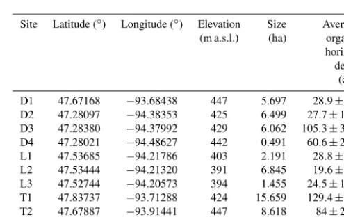
Table 1.Site information for 10 black ash study wetlands.
Site Latitude (◦) Longitude (◦) Elevation Size Average (m a.s.l.) (ha) organic horizon depth (cm) D1 47.67168 −93.68438 447 5.697 28.9±9.1 D2 47.28097 −94.38353 425 6.499 27.7±11.3 D3 47.28380 −94.37992 429 6.062 105.3±32.2 D4 47.28021 −94.48627 442 0.491 60.6±22.1 L1 47.53685 −94.21786 403 2.191 28.8±9.5 L2 47.53444 −94.21320 391 6.845 19.6±7.2 L3 47.52744 −94.20573 394 1.455 24.5±10.1 T1 47.83737 −93.71288 424 15.659 129.4±3.6 T2 47.67887 −93.91441 447 8.618 84±26.2 T3 47.27623 −94.48689 432 1.938 53.6±28.5
[image:3.612.307.555.360.516.2]Figure 2. Map of black ash wetland sites. Sites are colored by their mean organic horizon depth. Imagery provided by © Google Maps 2019.
late successional or climax communities and have not been harvested for at least a century.
As part of a larger effort to understand and characterize black ash wetlands (D’Amato et al., 2018), we categorized and grouped each wetland by its hydrogeomorphic charac-teristics as follows: (1) depression sites (“D”, n=4) char-acterized by a convex, pool-type geometry with geographi-cal isolation from other surface water bodies and surrounded by uplands; (2) lowland sites (“L”, n=3) characterized by extensive wetland complexes on flat, gently sloping topogra-phy; and (3) transition sites (“T”,n=3) characterized as flat, linear boundaries between uplands and black spruce (Picea marianaMill. Britton) bogs (Fig. 3). The three lowland sites were control plots from a long-term experimental random-ized block design on black ash wetlands (blocks 1, 3, and 6; Slesak et al., 2014; Diamond et al., 2018). We considered hydrogeomorphic variability among sites an important crite-rion, as it allowed us to capture expected differences in hy-drologic regime and, thus, differences in the strength of our predicted control on microtopographic generation (Fig. 1). Ground slopes across sites ranged from 0 % to 1 %. Black ash wetlands are typically hydrologically disconnected from regional groundwater and other surface water bodies, result-ing in precipitation and evapotranspiration (ET) as dominant components of the water budget, with no indication of ex-treme surface flows (Slesak et al., 2014). Water levels follow a common annual trajectory of late-spring/early-summer in-undation (10–50 cm) followed by ET-induced summer draw-down and belowground water levels (Slesak et al., 2014; Di-amond et al., 2018). However, the degree of drawdown de-pends on the local hydrogeomorphic setting; we observed
considerably wetter conditions at depression and transition sites than at lowland sites.
2.1.1 Vegetation
Overstory vegetation at the 10 sites is dominated by black ash, with tree densities ranging from 650 stems ha−1 (basal area of 195 m2ha−1) at the driest lowland site to 1600 stems ha−1(basal area of 40 m2ha−1) at a much wet-ter depression site (the across-site mean was 942 stems ha−1; Diamond et al., 2019). At the lowland sites, other overstory species were negligible, but at the depression and transi-tion sites there were minor cohorts of northern white cedar (Thuja occidentalisL.), green ash (Fraxinus pennsylvanica
Marshall), red maple (Acer rubrum L.), yellow birch ( Be-tula alleghaniensisBritt.), balsam poplar (Populus balsam-ifera L.), and black spruce (Picea marianaMill. Britton). Except at one transition site (T1), where northern white cedar represented a significant overstory component, black ash rep-resented over 75 % of overstory cover across all sites. Black ash also made up the dominant midstory component at each site, but was regularly found with balsam fir (Abies bal-sameaL. Mill.) and speckled alder (Alnus incanaL. Moench) in minor components, and greater abundances of American elm (Ulmus AmericanaL.) at lowland sites. Black ash stands are commonly highly uneven with respect to age (Erdmann et al., 1987), with canopy tree ages ranging from 130 to 232 years, and stand development under a gap-scale distur-bance regime (D’Amato et al., 2018). Black ash are also typ-ically slow-growing, achieving heights of only 10–15 m and diameters at breast height of only 25–30 cm after 100 years (Erdmann et al., 1987). The relatively open canopies of black ash wetlands (leaf area index<2.5; Telander et al., 2015) al-low for a variety of graminoids, shrubs, and mosses to grow in the understory. However, the majority of understory diver-sity and biomass tends to occur on hummocks that are oc-cupied by black ash trees (Diamond et al., 2019). Hollows exhibit relatively little plant cover and are typically bare soil areas, but may be covered at times of the year by sedges (Carexspp.) or layers of duckweed (Lemna minor L.), es-pecially after recent inundation.
2.1.2 Soils
Figure 3. (a–c)Photos of observed black ash wetland microtopography from a site in each hydrogeomorphic category:(a)depression site D2, (b)transition site T1, and(c)lowland site L3. Hummocks are outlined using yellow/orange dashed lines, and hollows are outlined and lightly shaded in blue. Lowland (L3) site hummocks and hollows are difficult to discern in summer time due to heavy understory cover and are additionally less pronounced, so they are not drawn here. In contrast, depression (D2) and transition (T1) site hummocks were typically more visually distinct from hollow surfaces.(d–f)Corresponding automatically delineated hummocks for every site with hill-shaded surface models in the background:(d)D2,(e)T1, and(f)L3. Hummocks are colored at each site using a unique identifier. Although some hummocks have similar colors to their neighbors, indicating that they are the same hummock, if they are separated by gray space (hollows), they are unique.
the deepest O horizons (>100 cm), and were associated with Typic Haplosaprists of the Seelyeville series and Typic Hap-lohemists (NRCS, 2019). Both depression and transition sites had much deeper O horizons than lowland sites, but depres-sion site organic soils were typically muckier and more de-composed than more peat-like transition site soils.
2.2 TLS
2.2.1 Data collection
To characterize the microtopography of our sites, we con-ducted a terrestrial laser scanning (TLS) campaign from 20 to 24 October 2017. We chose this period to ensure high-quality TLS acquisitions, as it coincided with the time of least vege-tative cover and the least likelihood for inundated conditions. During scanning, leaves from all deciduous canopy trees had fallen and grasses had largely senesced. Standing water was present at portions of three of the sites and was typically dispersed across the site in small pools (ca. 0.5–2 m2) less than 10 cm deep. We used a Faro Focus 120 3-D phase-shift TLS (905 nmλ) to scan three randomly established, 10 m di-ameter sampling plots at each site (see Stovall et al., 2019 for exact methodological details). For each site, we merged our plot-level TLS data to a single∼900 m2site-level point-cloud using 30 strategically placed and scanned 7.62 cm
ra-dius polystyrene registration spheres set atop 1.2 m stakes. We referenced each site to a datum located at each site’s base well elevation (see Sect. 2.3.1).
To validate the TLS surface model products, we installed sixty 2.54 cm radius spheres on fiberglass stakes exactly 1.2 m above ground surface at each site. Using the valida-tion locavalida-tions, we could easily calculate the exact surface el-evation (i.e., 1.2 m below a scanned sphere) of 60 points in space. We installed 39 (13 at each plot) validation spheres at points according to a random walk sampling design, and placed 21 (7 at each plot) validation spheres on distinctive hummock–hollow transitions. We placed the 1.2 m tall vali-dation spheres approximately plumb to reduce errors due to horizontal misalignment.
We processed the point clouds generated from the TLS sampling campaign to generate two products: (1) site-level 1 cm resolution ground surface models, and (2) site-level de-lineations of hummocks and hollows. The details and vali-dation of this method are described completely in Stovall et al. (2019), but a brief summary is provided here.
2.2.2 Surface model processing and validation
[image:5.612.70.528.66.292.2]moving 0.5 cm grid. We removed tree trunks from this initial surface model using a slope analysis and implemented a final outlier removal filter to ensure all points above ground level were excluded. Our final site-level surface models meshed the remaining slope-filtered point cloud using a local min-ima approach at a 1 cm resolution. We validated this final 1 cm surface model using the 60 validation spheres per site.
Before we analyzed surface models from each site, we first detrended sites that exhibited site-scale elevation gradi-ents (e.g., 0.02 cm m−1). These gradients may obscure anal-ysis of site-level relative elevation distributions (Planchon et al., 2002), and our hypothesis relates to relative elevations of hummocks and hollows and not their absolute elevations. We chose the best-detrended surface model based on ad-justedR2 values and observation of resultant residuals and elevation distributions from three options: no detrend, lin-ear detrend, and quadratic detrend. Five sites were detrended: L2 was detrended with a linear model; and D1, D2, D4, and T1 were detrended with quadratic models. We then subsam-pled each surface model to 10 000 points to speed up process-ing time, as the original surface models were approximately 100 000 000 points. We observed no significant difference in results from the original surface model based on our subsam-pling routine.
2.2.3 Hummock delineation and validation
We classified the final surface model into two elevation categories: hummocks and hollows. We first classified hol-lows using a combination of normalized elevation and slope thresholds; hollows have less than average elevation and less than average slope. This combined elevation and slope ap-proach avoided confounding hollows with the tops of hum-mocks as the tops of humhum-mocks are typically flat or shallow sloped. We removed hollows and used the remaining area as our domain of potential hummocks.
Within the potential hummock domain, we segmented hummocks into individual features using a novel approach – TopoSeg (Stovall et al., 2019) – and thereby created a hummock-level surface model for each site. We first used the local maximum (Roussel and Auty, 2018) of a moving window to identify potential microtopographic structures for segmentation. The local maximum served as the “seed point” from which we then applied a modified watershed delin-eation approach (Pau et al., 2010). The watershed delindelin-eation inverts convex topographic features and finds the edge of the “watershed”, which in our case are hummock edges. The de-fined boundary was used to clip and segment hummock fea-tures into individual hummock surface models.
For each delineated hummock within each site, we cal-culated the perimeter length, total area, volume, and height distributions relative to both local hollow datum and to a site-level datum. To calculate area, we summed the total number of points in each hummock raster multiplied by the model resolution (1 cm2). We calculated volume using the
same method as area, but multiplied by each points’ height above the hollow surface. The perimeter was conservatively estimated by converting our raster-based hummock features into polygons and extracting the edge length from each hum-mock. We estimated lateral hummock area by modeling each hummock as a simple cone, and calculating the lateral sur-face area from the previously estimated volume and height. We believe this conical estimation method to be a conserva-tive representation of the average height around the perimeter of the hummock because real hummock shapes are more un-dulating and complex than simple cones. We elected not to use a cylindrical model because we observed some tapering of hummocks from their base to their top. We note that a cylindrical model would increase lateral surface area estima-tion by approximately 15 % compared with the conical model and may therefore provide an upper bound for our conserva-tive estimates.
To validate the hummock delineation, we compared man-ually delineated and automatically delineated hummock size distributions at one depression site (D2) and one transition site (T1), both with clearly defined hummock features. We omitted using a lowland site for validation because none of these sites had obvious hummock features that we could manually delineate with confidence. We manually delineated hummocks for the D2 and T1 sites with a qualitative vi-sual analysis of raw TLS scans using the clipping tool in CloudCompare (2018). Stovall et al. (2019) found no signif-icant differences between the manual and automatically seg-mented hummock distributions, and feature geometry had an RMSE of less than approximately 20 %.
After the automatic delineation procedure and subsequent validation, we performed a data cleaning procedure by man-ually inspecting outputs in the CloudCompare software. We eliminated clear hummock mischaracterization that was es-pecially prevalent at the edges of sites, where point densi-ties were low. We also excluded downed woody debris from further hummock analysis because, although these features may serve as nucleation points for future hummocks, they are not traditionally considered hummocks and their distri-bution does not relate to our broad hypotheses. Finally, we excluded delineated hummocks that were less than 0.1 m2in area because we did not observe hummocks less than this size during our field visits. This delineation and manual cleaning process yielded point clouds of hummocks and hollows for every site, which could be further analyzed.
2.2.4 Surface model performance
point density or a complete absence of lidar returns. We ob-served overestimation of the surface model when TLS scans were unable to reach the ground surface, leading to the great-est overgreat-estimations at sites with dense grass cover (lowland sites). Overestimation was also common at locations with no lidar returns, such as small hollows, where the scanner’s oblique view angle was unable to reach. Nonetheless, exam-ination of the surface models indicated the clear ability of the TLS to capture surface microtopography (Fig. S1 in the Supplement).
2.2.5 Hummock delineation performance
Hummocks delineated from our algorithm were generally consistent in distribution and dimension with manually de-lineated hummocks. However, the automatic delineation lo-cated hundreds of small (<0.1 m2) “hummock” features that were not captured with manual delineation, which we at-tribute to our detrending procedure. We did not consider au-tomatically delineated hummocks less than 0.1 m2in further analyses, as we did not observe hummocks smaller than this in the field. Both area and volume size distributions from the manual and automatic delineations were statistically in-distinguishable for botht test (p value=0.84 and 0.51, re-spectively) and Kolmogorov–Smirnov test (p value=0.40 and 0.88, respectively). Automatically delineated hummock area, the perimeter : area ratio, and volume estimates had 23 %, 19.6 %, and 24.1 % RMSE values, respectively, and the estimates were either unbiased or slightly negatively bi-ased (−9.8 %, 0.2 %, and−11.9 %, respectively). We con-sider these errors to be well within the range of plausibility, especially considering the uncertainty involved in the man-ual delineation of hummocks, both in the field and on the computer. Final delineations showed clear visual differences among site types in the spatial distributions of hummocks (Fig. S2).
2.3 Field data collection 2.3.1 Hydrology
To address our hypothesis that hydrology is a controlling variable of microtopographic expression in black ash wet-lands, we instrumented all 10 sites to continuously moni-tor water level dynamics and precipitation. Three sites (L1, L2, and L3; Slesak et al., 2014) were instrumented in 2011 and seven in June 2016 following the same protocols. At each site, we placed a fully slotted observation well (sched-ule 40 PVC, 5 cm diameter, 0.025 cm wide slots) at approxi-mately the lowest elevation; at the flatter L sites, wells were placed at the approximate geographic center of each site. The ground surface at the well served as each site’s datum (i.e., elevation=0 m). We instrumented each well with a high-resolution total pressure transducer (HOBO U20L-04, reso-lution of 0.14 cm and average error of 0.4 cm) to record water
level time series at 15 min intervals. We dug each well with a hand auger to a depth associated with the local clay mineral layer and did not penetrate the mineral layer, which ranged from 30 cm below the soil surface to depths greater than 200 cm. We then backfilled each well with a clean, fine sand (20–40 grade). At each site, we also placed a dry well with the same pressure transducer model to measure temperature-buffered barometric pressure and frequency for barometric pressure compensation (McLaughlin and Cohen, 2011). 2.3.2 Mineral layer depth measurements
To quantify the control that underlying mineral layer micro-topography has on surface micromicro-topography, we conducted synoptic measurements of mineral layer depth and thus or-ganic soil thickness at each site. Within each of the 10 m di-ameter plots used for TLS at each site, we took 13 measure-ments (co-located with the randomly established validation spheres) of depth-to-mineral-layer using a steel 1.2 m rod. At each point the steel rod was gently pushed into the soil with consistent pressure until resistance was met and the depth to resistance was recorded (resolution of 1 cm) as the “mineral-layer”. We then associated each of these depth-to-mineral-layer measurements with a soil elevation based on TLS data and the site-level datum (i.e., elevation at the base of each site’s well).
2.4 Data analysis 2.4.1 Hydrology
We calculated simple hydrologic metrics based on the 3 years (2016–2018) of water level data for each site. For each site, we calculated the mean and variance of water level ele-vation relative to ground surface at the well, where negative values represent belowground water levels and positive val-ues indicate inundation. We also calculated the average hy-droperiod of each site by counting the number of days that the mean daily water level was above the soil surface at the well each year, and averaging across years.
2.4.2 Elevation distributions
sampling resolution to capture parameter variance at small scales. The larger the difference between the sill and the nugget (the “partial sill”), the more spatially predictable the parameter. If the semivariogram is entirely represented by the nugget (i.e., slope of 0), the parameter is randomly spatially distributed. The semivariogram range is the distance where the semivariogram reaches its sill, and it represents the spatial extent (patch size) of heterogeneity, beyond which data are randomly distributed. When spatial dependence is present, semivariance will be low at short distances, increase for inter-mediate distances, and reach its sill when data are separated by large distances. We used detrended elevation models for this analysis to more directly assess the importance of mi-crotopography on elevation variation as opposed to having it obscured by site-level elevation gradients. From these semi-variograms we calculated the best-fit semivariogram model among exponential, Matérn, or Matérn with Stein parame-terization model forms (Minasny and McBratney, 2005). We also extracted semivariogram nuggets, ranges, sills, and par-tial sills.
Our second line of inquiry was to evaluate the degree of elevation bimodality in these systems, which is indicative of a positive feedback between hummock growth and hummock height (Eppinga et al., 2008). Based on the classification into hummock or hollow from our delineation algorithm, we plotted site-level detrended elevation distributions for hum-mocks and hollows and determined a best-fit Gaussian mix-ture model with Bayesian information criteria (BIC) using the “mclust” package (Scrucca et al., 2016) in R (R Core Team, 2018), which uses an expectation-maximization algo-rithm. Mixture models were allowed to have either equal or unequal variance, and were constrained to a comparison of bimodal versus a unimodal mixture distribution.
2.4.3 Subsurface topographic control on microtopography
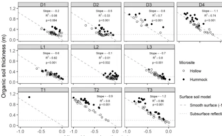
We assessed the importance of mineral layer microtopog-raphy on soil surface microtopogmicrotopog-raphy by comparing the depth-to-mineral-layer measurements with the soil surface elevation TLS measurements. We first calculated the eleva-tion of the mineral layer relative to each site-level datum by subtracting the depth-to-mineral-layer measurement from its co-located soil elevation measurement estimated from the TLS campaign. We then plotted the depth-to-mineral-layer measurement (hereafter referred to as “organic soil thick-ness”) as a function of this mineral layer elevation, noting which points were on hummocks or hollows as determined from the TLS delineation algorithm. We fit linear models to these points and compared the regression slopes to the ex-pected slopes from (1) a scenario where surface microto-pography is simply a reflection of subsurface microtopog-raphy (slope of 0, or constant organic soil thickness), and (2) a scenario of flat soil surface where organic soil thick-ness negatively corresponds to varying mineral layer
eleva-tion (slope of−1, or varying soil thickness). The first sce-nario would indicate that surface microtopography mimics subsurface microtopography, whereas the second would indi-cate organic matter/surface soil accumulation and smoothing over a varying subsurface topography. Observations above the−1:1 line would indicate surface processes that increase elevation above expectations for a flat surface.
2.4.4 Hydrologic controls on hummock height
To test our hypothesis that hydrology is a broad, site-level control on hummock height, we first regressed site mean hummock height against site mean daily water level. We also conducted a within-site regression of individual hummock heights against their local mean daily water level. To do so, we first calculated a local relative mean water level for each delineated hummock location by subtracting the elevation minimum of the hummock (i.e., the elevation at the base of the hummock) from the site-level mean water level elevation. This calculation assumes that the water level is flat across the site, which is likely valid for the high permeability organic soils at each site, low slopes (<1 %), and relatively small ar-eas that we assessed. This within-site regression allowed us to understand more local-scale controls on hummock height. 2.4.5 Hummock spatial distributions
To test whether there was regular spatial patterning of hum-mocks at each site, we compared the observed distribu-tion of hummocks against a theoretical distribudistribu-tion of hum-mocks subject to complete spatial randomness (CSR) with the R package “spatstat” (Baddeley et al., 2015). We first extracted the centroids and areas of the hummocks using TopoSeg (Stovall et al., 2019) and created a marked point pattern of the data. Using this point pattern, we conducted a nearest-neighbor analysis (Diggle, 2002), which evalu-ates the degree of dispersion in a spatial point process (i.e., how far apart on average hummocks are from each other). If hummocks are on average further apart (using the mean nearest-neighbor distance,µNN) compared with what would
be expected under CSR (µexp), the hummocks are said to be
overdispersed and subject to regular spacing; if hummocks are closer together than what CSR predicts, they are said to be underdispersed and subject to clustering. We compared the ratio ofµNN andµexp, where values greater than 1
in-dicate overdispersion and values below 1 inin-dicate cluster-ing, and calculated azscore (zANN) and subsequentpvalue
to evaluate the significance of overdispersion or clustering (Diggle, 2002; Watts et al., 2014). Thezscores were com-puted from the difference betweenµNN andµexp scaled by
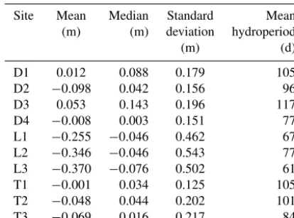
Table 2.Daily water level summary statistics for black ash study wetlands.
Site Mean Median Standard Mean
(m) (m) deviation hydroperiod
(m) (d)
D1 0.012 0.088 0.179 105
D2 −0.098 0.042 0.156 96
D3 0.053 0.143 0.196 117
D4 −0.008 0.003 0.151 77
L1 −0.255 −0.046 0.462 67
L2 −0.346 −0.046 0.543 77
L3 −0.370 −0.076 0.502 61
T1 −0.001 0.034 0.125 105
T2 −0.048 0.044 0.202 101
T3 −0.069 0.016 0.217 84
2.4.6 Hummock size distributions
To test the prediction that hummock sizes are constrained by patch-scale negative feedbacks, we plotted site-level rank-frequency curves (inverse cumulative distribution functions) for hummock perimeter, area, and volume. These curves trace the cumulative probability of a hummock dimension (perimeter, area, or volume) being greater than or equal to a certain value (P[X≥x]). We then compared best-fit power (P[X≥x] =αXβ), lognormal (P[X≥x] =βln(X)+β0),
and exponential (P[X≥x] =αeβX) distributions for these curves using AIC values. Power-scaling of these curves oc-curs where negative feedbacks to hummock size are con-trolled at the landscape-scale (i.e., hummocks have approxi-mately equal probability to be found at all size classes). Trun-cated scaling of these curves, as in the case of exponential or lognormal distributions, occurs when negative feedbacks to hummock size are controlled at the patch-scale (Scanlon et al., 2007; Watts et al., 2014).
3 Results 3.1 Hydrology
Hydrology varied across sites, but largely corresponded to hydrogeomorphic categories (Table 2). Depressions sites were the wettest sites (mean daily water level of−0.01 m), followed by transition sites (−0.04 m), and lowland sites (−0.32 m). Lowland sites also exhibited significantly more water level variability than transition or depression sites, whose water levels were consistently within 0.4 m of the soil surface. Although lowland sites exhibited greater water level drawdown during the growing season, they were able to rapidly rise after rain events.
3.2 Elevation distributions
Semivariograms demonstrated much more pronounced el-evation variability at depression and transition sites than at lowland sites (Fig. 4). In general, lowland sites reached overall site elevation variance (sills, horizontal dashed lines) within 5 m, but best-fit ranges (dotted vertical lines in Fig. 4) were less than 1 m. In contrast, best-fit semivariogram ranges for depression and transition sites were several times greater. Therefore, depression and transitions sites have much larger ranges of spatial autocorrelation for elevation than lowland sites. Semivariograms were all best fit with Matérn models with Stein parameterizations, and nugget effects were ex-tremely small in all cases (average<0.001), which we at-tribute to the very high precision of the TLS method. As such, partial sills were quite large (i.e., the difference be-tween the sill and nugget), indicating that very little elevation variation occurs at scales less than our surface model resolu-tion (1 cm); the remaining variaresolu-tion is found over site-level ranges of autocorrelation. We did not observe major differ-ences in directional semivariograms compared to the omni-directional semivariogram, implying isotropic variability in elevation, and do not present them here.
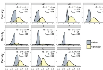
We observed bimodal elevation distributions at every site, with hummocks clearly belonging to a distinct elevation class separate from hollows (Fig. 5). Bimodal mixture models of two normal distributions were always a better fit to the data than unimodal models based on BIC values. Differences in mean elevations between these two classes ranged from 12 cm at the lowland sites to 20 cm at depression sites, and hummock elevations were more variable than hollow eleva-tions across sites. Across sites, 27 %±10 % of all elevations did not fall into either a hummock or a hollow category, with lowland sites having considerably more elevations not in these binary categories (36 %–44 %) compared with de-pression (22 %–27 %) or transition sites (16 %–22 %). How-ever, we emphasize that even when considering the entire site elevation distribution (i.e., including elevations that did not fall into a hummock or hollow category), bimodal fits were still better than unimodal fits, but to a lesser extent for low-land sites (Fig. S3). Delineated hummocks varied in number and size across and within sites. We observed the greatest number of hummocks at the depression and transition sites, with approximately an order of magnitude fewer hummocks found at lowland sites (Fig. 5).
3.3 Subsurface topographic control on microtopography
ex-Figure 4.Omnidirectional semivariograms for site elevations by hydrogeomorphic category (D refers to depression, L refers to lowland, and T refers to transition). Sites are colored according to their number within their hydrogeomorphic category. Dotted vertical lines indicate best-fit ranges, and horizontal dashed lines indicate best-fit partial sills (sill – nugget).
Figure 5.Relative elevation probability densities for each site, colored by hummock and hollow. The text indicates the difference in mean elevation (1z; m) between hummocks and hollows at each site (±SD – standard deviation), the total number of hummocks identified at each site (n), and the ratio of hummock area to total site area (Aratio). Depression sites (D) occupy the top row, followed by lowland sites (L), and
transition sites (T). Elevations are relative to the base of the well at each site, which was approximately the lowest elevation at each site.
cept for D1 and L2, there was a strong negative linear rela-tionship between soil thickness and mineral layer elevation, with five sites exhibiting slopes near −1, which we define as the smooth surface model of soil elevation (the dashed −1:1 line in Fig. 6). If only hollows (open circles; Fig. 6) were used in the regression, then D1 also exhibited a signif-icant (p <0.001) negative slope in this relationship (−0.4,
R2=0.52). A majority of the depth-to-mineral-layer mea-surements at D3 were below the detection limit with our 1.2 m steel rod, and all but one measurement at T1 were
[image:10.612.98.494.251.522.2]Figure 6.Organic soil thickness (measured as depth to resistance) as a function of mineral layer elevation. Points are filled by their microsite. The dashed (−1:1) line indicates a smooth surface soil model, and the dotted horizontal line indicates a subsurface reflection model. Text values are slopes,R2, andpvalues of the best-fit linear model for aggregated hummock and hollow points.
3.4 Hydrologic control on hummock height
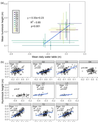
We observed a significant (p <0.001) positive linear rela-tionship between the site-level mean hummock height and the site-level mean daily water level (Fig. 7a). Because low-land sites were clearly influential points on this linear re-lationship, we also conducted this regression excluding the lowland sites and still found a significant (p=0.007) posi-tive linear trend between these variables with reasonable pre-dictive power (R2=0.8) – wetter sites have taller hummocks than drier sites on average. We found very little variability in the average hummock heights across sites relative to the site-level mean water site-level elevation (mean normalized hummock height of 0.31±0.06 m), indicating that hummocks were gen-erally about 30 cm higher than the site mean water level.
Within sites, we also observed clear positive relationships between individual hummock heights and their local mean daily water level (Fig. 7b). At all but two of the sites (D4 and L1), individual hummock heights within a site were sig-nificantly (p <0.01) taller at wetter locations than at drier locations. Slopes for these individual hummock regressions varied among sites, ranging from 0.4 to 1.1 (mean±SD of 0.7±0.2), and local hummock mean water level was able to explain 12 %–56 % (mean±SD of 0.36±0.14) of variability in hummock height within a site.
3.5 Hummock spatial distributions
All sites characterized as depressions or transitions exhibited a significant (p <0.001) overdispersion of hummocks com-pared with what would be predicted under complete spatial randomness (Fig. 8). For these sites, the nearest-neighbor ra-tios (µNN:µexp) indicated that hummocks are 25 %–30 %
further apart than would be expected with complete spa-tial randomness, with spacing of ca. 1.5 m, as evidenced by the narrow distributions in the nearest-neighbor histograms (Fig. 8). In contrast, all lowland sites, although they had hum-mock nearest-neighbor distances 2–3 times as far apart as depression or transition sites, were not significantly different from what would be predicted under complete spatial ran-domness (p values of 0.129, 0.125, 0.04 for sites L1, L2, and L3, respectively).
3.6 Hummock size distributions
simi-Figure 7.Hummock height as a function of mean water level.(a)Mean site-level hummock height (±SD) versus mean site-level daily water level (±SD), and(b)individual hummock height versus local daily mean water level. The slope,R2, andpvalues for the best-fit linear model (blue line) are presented.
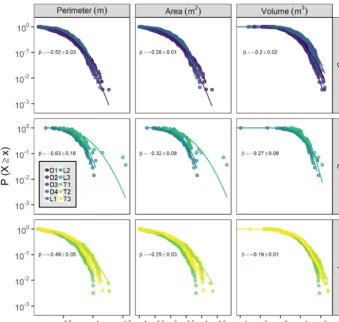
lar (Fig. 9). Lowland sites had significantly lower (p <0.05) coefficients for hummock property model fits than depres-sion or transition sites, with slopes that were approximately 20 % more negative on average, indicating more rapid trun-cation of size distributions. Across sites, the average hum-mock perimeter was 4.2±0.8 m, the average hummock area was 1.7±0.5 m2, and the average hummock volume was 0.17±0.06 m3. Hummock areas were typically less than 1 m2in size at all sites (Fig. 9). Similar to hummock spatial density, the hummock area per site (the ratio of hummock area to site area) was lower at drier lowland sites (2 %–5 %) compared with wetter depression and transition sites (12 %– 22 %) (Fig. 5).
4 Discussion
[image:12.612.129.470.64.488.2]Figure 8.Hummock nearest-neighbor distance distributions across sites. Bars are scaled density histograms overlaid with best-fit normal distributions (red lines). The text indicates the mean nearest-neighbor distance (µNN±SE – standard error); the ratio of the measured mean
nearest-neighbor distance and the expected nearest-neighbor distance for complete spatial randomness (µexp); and thepvalue for azscore
comparison betweenµNNandµexp.pvalues less than 0.001 indicate that hummocks are significantly overdispersed.
on microtopographic structure provide strong support for our hypothesis.
4.1 Controls on microtopographic structure
Bimodal soil elevation distributions at all sites suggest that the microsite separation into hummocks and hollows is a common attribute of black ash wetlands. Soil elevation bi-modality was most evident at the wetter depression and transition sites, where hummocks were more numerous and occupied a higher fraction of the overall site area (15 %– 20 %). Sharp boundaries between hummocks and hollows were not always observed in soil elevation probability den-sities (Fig. 5), which may be indicative of weak positive feedbacks between primary productivity and elevation (Ri-etkerk et al., 2004; Fig. 1). Conversely, modeling predic-tions indicate that if evapoconcentration feedbacks (i.e., that hummocks harvest nutrients from hollows through hydraulic gradients driven by hummock–hollow ET differences) are strong, boundaries between hummocks and hollows will be less sharp (Eppinga et al., 2009), possibly implicating mock evapoconcentration as an additional feedback to hum-mock maintenance (Fig. 1). Greater levels of soil chloride in hummocks relative to hollows in these systems may be an additional layer of evidence for this mechanism (Diamond et al., 2019).
Figure 9.Inverse cumulative distributions of hummock dimensions (perimeter, area, and volume) across sites (points), split by hummock dimension and site type. Theyaxis is the probability that a hummock dimension value is greater than or equal to the corresponding value on thexaxis. The best-fit lognormal distributions are shown for each site as lines. All fits were highly significant (p0.001). The text indicates the mean (±SD) within-group coefficient for a model of the formP (X≥x)=β·ln(dimension_value)+β0.
matter accumulation resulting from hypothesized elevation– productivity feedbacks.
Hummock heights relative to mean site-level water level were approximately 30 cm, aligning with field observations of relatively constant hummock height within sites. Gen-erally consistent hummock height across sites in conjunc-tion with clear bimodality in soil elevaconjunc-tions supports the contention that hummocks and hollows are discrete, self-organized ecosystem states (sensu Watts et al., 2010). How-ever, variability in site-level hummock heights – especially at depression and transition sites – may partially be attributable to hummocks in nonequilibrium states. From our feedback model (Fig. 1), it seems reasonable that within a site, some hummocks may be in growing states (e.g., increasing in height over time via the elevation–productivity positive feed-back) and some may be in shrinking states if hydrologic con-ditions have recently become drier (e.g., decreasing in height via the elevation–respiration negative feedback), the combi-nation of which may result in a distribution of hummock heights centered around an equilibrium hummock height. Fu-ture efforts could leverage time-series observations of
hum-mock properties (e.g., area, height, and volume), but we note the likely decadal timescales required to detect hummock growth or shrinkage (Benscoter et al., 2005; Stribling et al., 2007).
for hydrology. The flat water level assumption is likely to be a minor effect in transition sites with deep organic wet-land soils (e.g., Nungesser, 2003; Wallis and Raulings, 2011; Cobb et al., 2017) but could be significant at depression and lowland sites with shallower O horizons. A lack of sufficient data to characterize mean water level may also be an issue at several of our sites, because hummocks likely develop over the course of decades or longer, whereas our hydrology data only span 3 years. To our knowledge, this study represents the first empirical evidence of the positive relationship be-tween hummock height and hydrology in forested wetlands. These results are consistent with previous research on tus-socks of northern wet meadows (Peach and Zedler, 2006; Lawrence and Zedler, 2011) and shrub hummocks in brack-ish wetlands (Wallis and Raulings, 2011). The concordance in hydrologic control in these disparate systems suggests a common mechanism of (organic) soil building and accumu-lation on hummocks that may result from increased vegeta-tion growth from reduced water stress and/or from transport and accumulation of nutrients (Eppinga et al., 2009; Sullivan et al., 2008; Heffernan et al., 2013; Harris et al., 2019).
4.2 Controls on microtopographic patterning
We found clear support for our hypothesis that hummocks are non-randomly distributed in our wettest study sites. Hum-mocks exhibited spatial overdispersion at all sites, but this overdispersion was only significant at depression and transi-tion sites (Fig. 8). Significant spatial overdispersion indicates regular hummock spacing in contrast to clustered distribu-tions or completely random placement. Regular patterning of landscape elements is observed across climates, regions, and ecosystems (Rietkerk and Van de Koppel, 2008), and is indicative of negative feedbacks that limit patch expan-sion (Quinton and Cohen, 2019). Our results indicate similar patterning for forested wetland microtopography and, impor-tantly, demonstrate the hydrologic controls on that pattern-ing. Hydrology appears to be a common driver in regular pattern formation in wetlands (Heffernan et al., 2013) and drylands (Scanlon et al., 2007). Thus, water stress – both too much (Eppinga et al., 2009) and too little (Deblauwe et al., 2008; Scanlon et al., 2007) – appears to be an important reg-ulator of patch distribution across the landscape.
We observed lognormal hummock size distributions, sug-gesting that some hummocks may attain very large areas (i.e., over 10 m2), but the majority of hummocks (∼80 %) are less than 1 m2(Fig. 9). This finding aligns with field observations, where most hummocks were associated with a single black ash tree, but some hummocks appeared to have merged to create large patches. Truncated patch size distributions are common in other systems as well, such as the stretched ex-ponential distribution for geographically isolated wetlands (Watts et al., 2014) or the lognormal distribution for desert soil crusts (Bowker et al., 2013). These types of distribu-tions have fewer large patches than would be expected for
systems without patch-scale negative feedbacks, and have a central tendency towards a common patch size. Hence, trun-cation in hummock size distributions comports with hypoth-esized patch-scale negative feedbacks (i.e., tree competition for light and/or nutrients) that inhibit expansion. Hummocks at drier lowland sites did not conform to size distributions for wetter depression and transition sites, supporting our hy-pothesis that the feedbacks that control hummock mainte-nance and distribution are governed by hydrology and am-plified in wetter conditions. This work adds to recent efforts across climates and systems to use patch size distributions to infer drivers of ecosystem self-organization and response to environmental conditions (Kéfi et al., 2007; Maestre and Es-cudero, 2009; Weerman et al., 2012; Schoelynck et al., 2012; Tamarelli et al., 2017).
4.3 Evidence for patch self-organization
In this work, we used common landscape ecology diagnos-tics to characterize microtopographic patterns and infer the responsible reinforcing processes, including analyses of mul-timodal distributions of elevation, spatial patterns of hum-mock patches, and humhum-mock size distributions. Other re-cent work has used nearly identical diagnostic measurements to infer self-organization of depressional wetland features (∼100 m wide) in a karst landscape (Quinton and Cohen, 2019), demonstrating the broad utility of the approach and the various spatial scales that patterns may manifest. How-ever, we note that this diagnostic approach alone does not di-rectly implicate hypothesized mechanisms of hummock per-sistence, and that more measurements are required to support inferences made here. To that end, in complementary work we observed support for the elevation–productivity feedback, where we found hummocks to be loci of higher tree occur-rence and biomass, more understory diversity, and greater phosphorus and base cation soil concentrations (Diamond et al., 2019). Furthermore these associations were most evident at the wettest sites, concordant with the hydrologic controls observed here for hummock height, pattern, and size distribu-tions. Together, these multiple lines of evidence lend strong support for the hydrologically driven self-organization hy-pothesis of hummock growth and persistence (Fig. 1).
4.4 Broader implications
The consequences of wetland microtopography are clear at small scales, but can also scale to influence site- and regional-scale processes. For example, microtopographic expression results in a drastic increase in surface area within wetlands. We conservatively estimate an average of 22 % and up to a 42 % relative increase in surface area due to the presence of hummocks (i.e., additional surface area provided by the sides of hummocks; Table 3). These estimates comport with stud-ies in tussock meadows, where tussocks (ca. 20 cm tall) in-creased surface area by up to 40 % (Peach and Zedler, 2006). Furthermore, increases in the diversity of biogeochemical processes occurring at the individual hummock or hollow scale (Deng et al., 2014) likely aggregate to influence ecosys-tem functioning at large scales. For example, microtopo-graphic niche expansion allows for local material and solute exchange between hummocks and hollows, creating coupled aerobic–anaerobic conditions with emergent outcomes for denitrification (Frei et al., 2012) and carbon emission (Bu-bier et al., 1995; Minick et al., 2019a, b).
[image:16.612.308.546.86.274.2]While our results implicate hydrology as a major deter-minant of microtopographic structure and pattern, microto-pography can reciprocally influence system-scale hydraulic properties. Results from our hummock property analysis in-dicate that hummock volume displacement may be a signif-icant factor in water level dynamics of wetlands. Specific yield, which governs the water level response to hydrologic
Table 3.Relative area increase by hummocks across sites.
Site Survey Hummock Relative
area side surface area
(m2)a area (m2)b increase by hummocks
D1 1045 267 0.26
D2 1041 258 0.25
D3 1093 311 0.28
D4 1164 217 0.19
L1 1234 92 0.07
L2 919 34 0.04
L3 1221 56 0.05
T1 731 304 0.42
T2 994 376 0.38
T3 1198 308 0.26
Average 222±114 0.22±0.13
(Average, no L)c (291±47) (0.29±0.07)
aSurvey area is the area scanned by TLS.bHummock side surface area is
calculated from measured volumes and heights using a cone model.c“Average no-L” refers to the same summary statistics but excluding L sites (L1, L2, and L3) from the calculation.
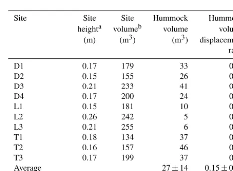
Table 4.Hummock volume displacement ratios for all sites.
Site Site Site Hummock Hummock heighta volumeb volume volume (m) (m3) (m3) displacement ratio
D1 0.17 179 33 0.18
D2 0.15 155 26 0.17
D3 0.21 233 41 0.18
D4 0.17 200 24 0.12
L1 0.15 181 10 0.05
L2 0.26 242 5 0.02
L3 0.21 255 6 0.02
T1 0.18 134 37 0.28
T2 0.16 157 46 0.30
T3 0.17 199 37 0.18
Average 27±14 0.15±0.09 (Average, no L) (35±7) (0.20±0.06)
aSite height is estimated as the mean 80th percentile of hummock heights across the site. bSite volume is estimated by multiplying site height by site area.
fluxes, is commonly assumed to be unity when wetlands are inundated. However, inclusion of microtopography may ren-der this assumption invalid, with hummock volumes up to 30 % of site volumes (Table 4). These observations are sup-ported in other studies of microtopographic effects of spe-cific yield (Sumner, 2007; McLaughlin and Cohen, 2014; Dettmann and Bechtold, 2016). Therefore, while hydrology exerts clear control on the geometry of hummocks, hum-mocks may exert reciprocal control on hydrology by am-plifying small hydrologic fluxes into large water level vari-ations.
[image:16.612.309.544.349.521.2]diver-sity (Diamond et al., 2019), aligning with observations in other wetland systems (Bledsoe and Shear, 2000; Peach and Zedler, 2006; Økland et al., 2008). Accordingly, recent wet-land restoration efforts have begun to use microtopography as a strategy to promote seedling success and long-term project viability (Larkin et al., 2006; Bannister et al., 2013; Lieffers et al., 2017). Specific to our focal system, there are increasing efforts to mitigate potential black ash loss due to the emerald ash borer and possible regime shifts to marsh-like states (Diamond et al., 2018). We posit that hummock presence and persistence may allow for future tree seedlings to survive wetting up periods following this ash loss (Sle-sak et al., 2014), and for consequent resilience of forested ecosystem states.
Overall, this study adds to the growing body of evidence that the structure and regular patterning of wetland microto-pography is an autogenic response to hydrology. Although the imprint of biota on landscapes may be masked by the sig-nature of larger-scale physical processes (Dietrich and Per-ron, 2006), we show clear evidence here for a microtopo-graphic signature of life.
Code and data availability. Code for analysis and figure creation is available at https://doi.org/10.5281/zenodo.3571857 (Diamond, 2019).
Supplement. The supplement related to this article is available on-line at: https://doi.org/10.5194/hess-23-5069-2019-supplement.
Author contributions. JSD and DLM created the conceptual frame-work, questions, and hypotheses. AS and JSD developed the TLS procedure and carried out measurements and subsequent anal-ysis/coding; JSD and RAS carried out hydrology measurements. JSD conducted all data analysis and wrote the paper. All co-authors contributed significantly to editing the paper.
Competing interests. The authors declare that they have no conflict of interest.
Acknowledgements. We gratefully acknowledge the field work and data collection assistance provided by Mitch Slater, Alan Toczyd-lowksi, and Hannah Friesen. The authors also acknowledge two anonymous reviewers and Victor Lieffers, whose comments and suggestions improved this paper.
Financial support. This project was funded by the Minnesota En-vironmental and Natural Resources Trust Fund, the USDA For-est Service Northern Research Station, and the Minnesota ForFor-est Resources Council. Additional funding was provided by the Vir-ginia Tech Forest Resources and Environmental Conservation de-partment, the Virginia Tech Institute for Critical Technology and
Applied Science, and the Virginia Tech William J. Dann Fellowship. Jacob S. Diamond is supported by POI FEDER Loire no. 2017-EX001784, the Water Agency of Loire Catchment AELB, and the University of Tours.
Review statement. This paper was edited by Sally Thompson and reviewed by two anonymous referees.
References
Baddeley A., Rubak, E., and Turner, R.: Spatial Point Pat-terns: Methodology and Applications with R, Chapman and Hall/CRC Press, London, available at: http://www.crcpress.com/ Spatial-Point-Patterns-Methodology-and-Applications-with-R/ Baddeley-Rubak-Turner/9781482210200/ (last access: 13 December 2019), 2015.
Bannister, J. R., Coopman, R. E., Donoso, P. J., and Bauhus, J.: The Importance of Microtopography and Nurse Canopy for Success-ful Restoration Planting of the Slow–Growing Conifer Pilgero-dendron uviferum, Forests, 4, 85–103, 2013.
Benscoter, B. W., Kelman Wieder, R., and Vitt, D. H.: Linking mi-crotopography with post-fire succession in bogs, J. Veg. Sci., 16, 453–460, 2005.
Bertolini, C., Cornelissen, B., Capelle, J., Van De Koppel, J., and Bouma, T. J.: Putting self-organization to the test: labyrinthine patterns as optimal solution for persistence, Oikos, 128, 1805– 1815, https://doi.org/10.1111/oik.06373, in press, 2019. Bledsoe, B. P. and Shear, T. H.: Vegetation along hydrologic and
edaphic gradients in a North Carolina coastal plain creek bottom and implications for restoration, Wetlands, 20, 126–147, 2000. Bowker, M. A., Maestre, F. T., and Mau, R. L.: Diversity and
patch–size distributions of biological soil crusts regulate dryland ecosystem multifunctionality, Ecosystems, 16, 923–933, 2013. Bubier, J. L., Moore, T. R., Bellisario, L., Comer, N. T., and Crill,
P. M.: Ecological controls on methane emissions from a north-ern peatland complex in the zone of discontinuous permafrost, Manitoba, Canada, Global Biogeochem. Cy., 9, 455–470, 1995. CloudCompare (version 2.10.1): GPL software, available at: http:
//www.cloudcompare.org/, last access: 1 January, 2018. Cobb, A. R., Hoyt, A. M., Gandois, L., Eri, J., Dommain, R., Salim,
K. A., and Harvey, C. F.: How temporal patterns in rainfall deter-mine the geomorphology and carbon fluxes of tropical peatlands, P. Natl. Acad. Sci. USA, 114, E5187–E5196, 2017.
D’Amato, A., Palik, B., Slesak, R., Edge, G., Matula, C., and Bron-son, D.: Evaluating Adaptive Management Options for Black Ash Forests in the Face of Emerald Ash Borer Invasion, Forests, 9, 348, https://doi.org/10.3390/f9060348, 2018.
Deblauwe, V., Barbier, N., Couteron, P., Lejeune, O., and Bogaert, J.: The global biogeography of semi-arid periodic vegetation pat-terns, Global Ecol. Biogeogr., 17, 715–723, 2008.
Dettmann, U. and Bechtold, M.: One-dimensional expression to cal-culate specific yield for shallow groundwater systems with mi-crorelief, Hydrol. Process., 30, 334–340, 2016.
Diamond, J. S.: First release of code for microtopography, Zenodo, https://doi.org/10.5281/zenodo.3571857, 2019.
Diamond, J. S., McLaughlin, D. L., Slesak, R. A., D’Amato, A. W., and Palik, B. J.: Forested versus herbaceous wetlands: Can management mitigate ecohydrologic regime shifts from invasive emerald ash borer?, J. Environ. Manage., 222, 436–446, 2018. Diamond, J. S., McLaughlin, D. L., Slesak, R. A., and
Stovall, A.: Microtopography is a fundamental organizing structure in black ash wetlands, Biogeosciences Discuss., https://doi.org/10.5194/bg-2019-302, in review, 2019.
Dietrich, W. E. and Perron, J. T.: The search for a topographic sig-nature of life, Nature, 439, 411–418, 2006.
Diggle, P. J.: Statistical Analysis of Spatial Point Patterns, 2nd Edn., Hodder Education, London, 288 pp., 2002.
Duberstein, J. A., Krauss, K. W., Conner, W. H., Bridges Jr., W. C., and Shelburne, V. B.: Do Hummocks Provide a Physiological Advantage to Even the Most Flood Tolerant of Tidal Freshwater Trees?, Wetlands, 33, 399–408, 2013.
Eppinga, M. B., Rietkerk, M., Borren, W., Lapshina, E. D., Bleuten, W., and Wassen, M. J.: Regular surface patterning of peatlands: confronting theory with field data, Ecosystems, 11, 520–536, 2008.
Eppinga, M. B., De Ruiter, P. C., Wassen, M. J., and Rietkerk, M.: Nutrients and hydrology indicate the driving mechanisms of peatland surface patterning, Am. Nat., 173, 803–818, 2009. Erdmann, G. G., Crow, T. R., Ralph Jr., M., and Wilson, C. D.:
Managing black ash in the Lake States, General Technical Re-port NC-115, Department of Agriculture, Forest Service, North Central Forest Experiment Station, St. Paul, MN, USA, 115 pp., 1987.
Ettema, C. H. and Wardle, D. A.: Spatial soil ecology, Trends Ecol. Evol., 17, 177–183, 2002.
Franco, M.: The influence of neighbours on the growth of modu-lar organisms with an example from trees, Philos. T. Roy. Soc. Lond. B, 313, 209–225, 1986.
Frei, S., Knorr, K. H., Peiffer, S., and Fleckenstein, J. H.: Surface micro-topography causes hot spots of biogeo-chemical activity in wetland systems: A virtual model-ing experiment, J. Geophys. Res.-Biogeo., 117, G00N12, https://doi.org/10.1029/2012JG002012, 2012.
Gräler, B., Pebesma, E., and Heuvelink, G.: Spatio-Temporal Inter-polation using gstat, R Journal, 8, 204–218, 2016.
Harris, L. I., Roulet, N. T., and Moore, T. R.: Mechanisms for the Development of Microform Patterns in Peatlands of the Hudson Bay Lowland, Ecosystems, 1–27, 2019.
Heffernan, J. B., Watts, D. L., and Cohen, M. J.: Discharge com-petence and pattern formation in peatlands: a meta-ecosystem model of the Everglades ridge-slough landscape, PloS One, 8, e64174, https://doi.org/10.1371/journal.pone.0064174, 2013. Huenneke, L. F. and Sharitz, R. R.: Substrate heterogeneity and
re-generation of a swamp tree, Nyssa aquatic, Am. J. Bot., 77, 413– 419, 1990.
Jones, R. H., Lockaby, B. G., and Somers, G. L.: Effects of mi-crotopography and disturbance on fine-root dynamics in wetland forests of low-order stream floodplains, American Midland Nat-uralist, 136, 57–71, 1996.
Jones, R. H., Henson, K. O., and Somers, G. L.: Spatial, seasonal, and annual variation of fine root mass in a forested wetland, J. Torrey Bot. Soc., 127, 107–114, 2000.
Karban, R.: Plant behaviour and communication, Ecol. Lett., 11, 727–739, 2008.
Kéfi, S., Rietkerk, M., Alados, C. L., Pueyo, Y., Papanastasis, V. P., ElAich, A., and De Ruiter, P. C.: Spatial vegetation patterns and imminent desertification in Mediterranean arid ecosystems, Nature, 449, 213–217, 2007.
Kéfi, S., Rietkerk, M., Roy, M., Franc, A., De Ruiter, P. C., and Pascual, M.: Robust scaling in ecosystems and the meltdown of patch size distributions before extinction, Ecol. Lett., 14, 29–35, 2011.
Kéfi, S., Guttal, V., Brock, W. A., Carpenter, S. R., Ellison, A. M., Livina, V. N., Seekell, D. A., Scheffer, M., van Nes, E. H., and Dakos, V. Early warning signals of ecological tran-sitions: methods for spatial patterns, PloS one, 9, e92097, https://doi.org/10.1371/journal.pone.0092097, 2014.
Kurmis, V. and Kim, J. H.: Black ash stand composition and struc-ture in Carlton County, Minnesota, University of Minnesota, Re-port no. 69, 1989.
Larkin, D. J., Vivian-Smith, G., and Zedler, J. B.: Topographic het-erogeneity theory and ecological restoration, in: Foundations of restoration ecology, edited by: Falk, D. A., Palmer, M. A., and Zedler, J. B., Island Press, Washington, DC, USA, 2006. Lawrence, B. A. and Zedler, J. B.: Formation of tussocks by sedges:
effects of hydroperiod and nutrients, Ecol. Appl., 21, 1745–1759, 2011.
Lieffers, V. J., Caners, R. T., and Ge, H.: Re-establishment of hum-mock topography promotes tree regeneration on highly disturbed moderate-rich fens, J. Environ. Manage., 197, 258–264, 2017. Long, J. N. and Smith, F. W.: Volume increment in Pinus contorta
var. latifolia: the influence of stand development and crown dy-namics, Forest Ecol. Manage., 53, 53–64, 1992.
Maestre, F. T. and Escudero, A.: Is the patch size distribution of veg-etation a suitable indicator of desertification processes?, Ecology, 90, 1729–1735, 2009.
Manor, A. and Shnerb, N. M.: Facilitation, competition, and vegeta-tion patchiness: from scale free distribuvegeta-tion to patterns, J. Theor. Biol., 253, 838–842, 2008.
McLaughlin, D. L. and Cohen, M. J.: Thermal artifacts in mea-surements of fine-scale water level variation, Water Resources Research, 47, W09601, https://doi.org/10.1029/2010WR010288, 2011.
McLaughlin, D. L. and Cohen, M. J.: Ecosystem specific yield for estimating evapotranspiration and groundwater exchange from diel surface water variation, Hydrol. Process., 28, 1495–1506, 2014.
Miao, G., Noormets, A., Domec, J. C., Trettin, C. C., McNulty, S. G., Sun, G., and King, J. S.: The effect of water level fluctuation on soil respiration in a lower coastal plain forested wetland in the southeastern US, J. Geophys. Res.-Biogeo., 118, 1748–1762, 2013.