Impact of Integrating Wind Energy into Power Grid System

Impact of Integrating Wind Energy into Power Grid

System

Yasir Ghazi Rashid

Electrical Engineering Department University of Baghdad

Firas Mohammed Tuaimah,

University of Baghdad

ABSTRACT

Wind is one kind of free energy and this “must-take” wind power generation is integrated into the system operation. The optimal power flow (OPF) problem with integration wind energy was explored and exploited in this paper. This paper presents the impact integration wind wnergy on different performance parameters of power systems such as the total generation cost, voltage profile, power flow and power losses, by optimally integrate the wind farm in power systems. The modified IEEE 30 system with six thermal generating units and two wind farms. Several scenarios were conducted to determine the impact of single and multiple wind farm on the performance of the IEEE 30 bus system. In this paper, using programming language (Matlab) and PowerWorld software Version 19 to get the results.

Keywords

Optimal Power Flow, wind power, linear programming, voltage profile, PowerWorld.

1.

INTRODUCTION

Because wind power does not generate any emissions, it has been promoted as a clean way to generate electricity, with a variety of government policies encouraging its use [1]. In latest years, global wind energy has evolved hastily. Wind power capacity worldwide reaches 597 GW, 50.1 GW added in 2018. [2].Using the optimal power flow calculation (OPF) we can discover the impact of renewable energy on energy systems. The OPF is an important tool that system operators require to operate the network with a high penetration of wind power more efficiently, keeping all restrictions within tight limits.The OPF optimizes the static operating conditions of a power generation transmission system. The main advantages of the optimal energy flow are: (i) guaranteeing the static safety of the service quality by imposing limits on the operation of the generation transmission system, (ii) optimizing the voltage / reactive power planning and (iii) improving The operation economy through the full use of the eligible operating range of the system and the precise coordination of transmission losses in the planning process [3].

The objectives of this paper include studying the impact of the wind power penetration on as voltage profile, power flow of transmission lines, and reduction of the active and reactive power losses.

2.

THE GRID INTEGRATION OF

LARGE SCALE WIND

GENERATORS

In the coming years there will be an elementary change in the composition of the generation as a result of the need to replace many power plants due to aging. In this situation, the specific growth of renewable and dispersed generation plays

financed by fixed high-level prices for various renewable energy sources (RPS). These prices are independent of the network level in which RPS connections are provided. In-feed of power via large wind farms is essentially difficulty to different patterns as is the case with conventional power sources together with thermal, gas turbine or hydroelectric generating plants. Three essential problems need to be solved for the combination of huge wind farms in transmission system: (1) wind strength output relies upon on meteorological situations and can be intermittent. (2) A higher level of reserve strength than before ought to be furnished. (3) Suitable transmission capacities have to be created in order for the strength to reach the load facilities. Wind power manufacturers are entitled to switch their manufacturing to the gadget thru the electricity distribution or transmission business enterprise whenever the absorption of the strength via the network is “technically feasible” [4].

3.

PROBLEM FORMULATION

3.1

Mathematical Formulation

The OPF hassle incorporating wind power is the trouble to be studied in this paper and the planned wind energy blended with the power output of thermal electricity plant are as the variables to be optimized. Keep in mind that, the unbiased device operator might be accountable for the dispatching of wind strength and decide the corresponding power price.

The usual OPF problem can be formulated as a restrained optimisation problem as follows [5]

Minimize,

f1 (x,u)

F(x,u)= . where k= 1,2. No of objective

fk (x,u)

Subject to:

g(x,u)=0

h (x,u)≤0

Here x and u represent vector of dependent and control variables respectively. For example, the dependent variables represent slack bus power, bus voltage angles, load bus voltage magnitudes etc whereas PV bus voltage magnitude, generated power, tap position of tap changers, shunt compensators etc are represented by the control variables. g(x, u) denotes the real and reactive power balance equations and h(x, u) represents network or components operational limits.

3.2

Objective Functions

3.2.1

Fuel Cost

constraints. The generator cost curve that's a feature of strength output, may be represented by using the following quadratic equation.

F (P)

where n is the number of generators; aj , bj , cj are the fuel cost coefficients, ej and fj are fuel cost coefficients of the jth unit with valve points effects and Pj is the real power generated by the jth unit[6].

3.2.2

Active and Reactive Power Loss

The objective is to minimize the total active and reactive power losses in the transmission lines may be expressed as follows:

PL

QL

Where m is the total number of lines in the system; Gk is the conductance of the kth line; Bk is the susceptance of the kth line; Vi is the voltage magnitude at bus i; Vj is the voltage magnitude at bus j; δi is the voltage angle at bus i; δi and is the voltage angle at bus j [7].

3.2.3

Voltage Deviation

To have a good voltage performance, the voltage deviation at every load bus have to be made as small as possible. The voltage deviation (∆v) to be minimized is given in [8].

Where NPQ is the number of load buses and the desired or target value of the voltage magnitude at load bus k.

3.3

Constraints

3.3.1

Overloaded Lines

This objective is to minimize the power flow in overloaded transmission lines; this objective is calculated for every line of the system. The lines loading have to be less than one 100%. The active power and reactive power flow on lines can be applied as follows:

PGi

(6)

QGi

(7)

Where P is the real power generation at bus i; PDi is the real power demand at bus i; QDi is the reactive power generation at bus i; QDi is the reactive power demand at bus i; m is the total number of buses in the system; Vi is the voltage magnitude at bus i; Vi is the voltage magnitude at bus j; is the conductance of the kth line; is the susceptance of the kth line; δi is the voltage angle at bus i; and δj is the voltage angle at bus j[9].

3.3.2

Generation capacity constraints

The real power output of generating units have be restricted within their respective lower and upper bounds (inequality constraints) as follows:

Where n is the no of generators. and are minimum and maximum power outputs of jth generating unit respectively.

3.3.3

Other constraints

The other operational constraints involved in OPF problem are generator reactive power, voltages of all PV buses, transformer tap positions, VAR compensator position, bus voltage magnitudes of all PQ buses etc. These constraints can be formulated as follows:

Where nPV and nPQ are the number of PV buses and PQ buses respectively. nT and nC are the number of tap changing

transformer and switchable VAR compensator

respectively[10].

4.

OPTIMAL POWER FLOW (OPF)

Optimal power flow (OPF) problem has been one in all the foremost wide studied subjects within the power grid community since Carpentier 1st revealed the conception in 1962. The objective of optimum Power Flow (OPF) algorithm is to search out a gentle state operation purpose that minimizes generation price, network loss etc. or maximizes welfare or system utilization etc. even as preserving an acceptable system overall performance in phrases of limits on generators’ active and reactive powers, line go with the flow limits, most output of numerous compensating devices and many others.. Take optimum active power dispatch as associate degree example, the target operate is to attenuate total generation price or network losses whereas the system is working at intervals its security limits [11].

5.

LINEAR PROGRAMMING OPF

The early LP - based OPF method was restricted to network constrained economic power dispatch. The earliest versions used the fixed constraint approximations, primarily based on the purely dc power flow. In a while, incremental formulations have been brought, wherein constraint linearization is iterated with ac energy glide, to model and put into effect the constraints precisely. The benefits of the LP based OPF are:

1. Reliability of the optimization

2. Capability to recognize trouble infeasibility quick, in order that suitable strategies can be positioned into impact

3. The variety of operational limits can be easily accommodated and handled, together with contingency constraints

6.

INCREMENTAL LINEAR

PROGRAMMING METHOD

Studies have shown that the progressive linear programming (LP) technique will be accurately applied to a large vary of applications, and might manufacture a similar results as information NLP methods on power systems of every kind and sizes. Several benefits of the incremental LP technique over different existing strategies encompass its reliability, its ability to quickly understand trouble infeasibility, its capacity to deal with a wide range of operating limits, a very speedy computational speed, and extra flexibility for change-offs between computing speed and convergence accuracy. The incremental LP method is performed by linearizing the Fig.1.

= ( )

(15)

= ( )

16)

= 0

= 0

= 0

= 0

Constraint (12) represents the linearized real power equality constraints, (13) the linearized reactive power equality constraints, (14)-(17) the additional constraints on the swing bus and the load bus variables respectively for the problem to solve correctly, (18) the generator real power limits, (19) the generator reactive power limits, (20) the bus voltage magnitude limits, and (21)-(24) the size of the optimization region for each variable for the current iteration k. It should be noted that constraints (18)-(20) and (21)-(23) are overlapping. Thus, the constraints (18)-(20) will only be active if their corresponding variables ΔPgeni , ΔQgeni , or Δ|Vi| are at one of their limits. Otherwise, the variables will be free to move within the optimization region as specified in (21)- (23)[12].

Fig 1: Incremental LP method [14]

7.

CASE STUDY

Table 1. Test System Data

Generators 6

Buses 30

Load points 21

Total generation capacity 435MW

Fixed load 283.4 MW

The modified IEEE 30 system with six thermal generating units' two wind farms as shown in Fig.2. The wind power penetration level in this paper is defined as the ratio of the installed wind generation capacity to the total-installed system generation capacity of 10% (the installed wind generation capacity is 40 MW). Two wind farms including 10 wind generators each one have rating 2 MW (Type 4: Enercon E82 2MW) and connected at bus no. 10 and bus no. 24 (20 MW in each bus) is used to analyse the effect of connected wind farm on the total generation cost, voltage profile, power flow of transmission lines, the active and reactive power losses. Several scenarios with dispersed wind penetration levels from 0% to 100% have been investigated. The wind generators are connected at bus 10 and bus 24. The basic system data are

7.1

OPF Results without the Insertion of

Wind Farms

The results including the generation cost, the minimum deviation and power losses in the case without the penetration of the Wind generators are tabulated in Table 2.

Solve AC Power Flow Equation

Linearize Objective

Linearize Constraints

Set Variable Limits

Setup and Solve LP for New Control Variable Setting

Convergence Test

Converged

No significant movement of control variables Not converged

Significant movement of control

Table 2. Results of minimum total cost for IEEE 30-bus system by LPOPF

Variable PowerWorld Matlab

Pg1(MW) 196.351 195.6439

Pg2(MW) 44 43.8668

Pg5(MW) 22 21.4574

Pg8(MW) 10 10.5771

Pg11(MW) 10 10.0866

Pg13(MW) 12 12.0000

Production cost ($/hr) 803.91 803.26

Power Loss (MW) 10.54 10.31

Power Loss (Mvar) 21.23 19.67

7.2

Impact of Single Wind Farm Site

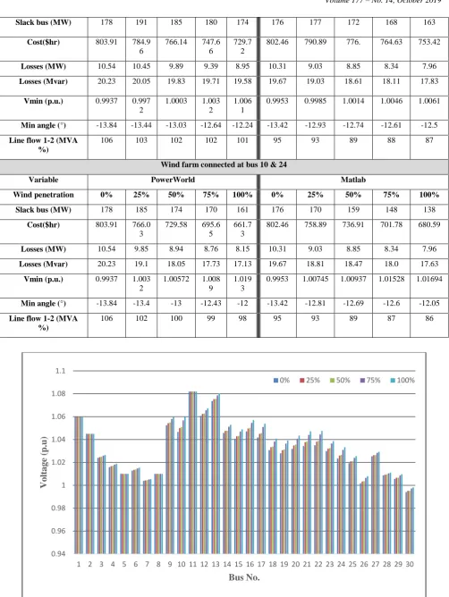
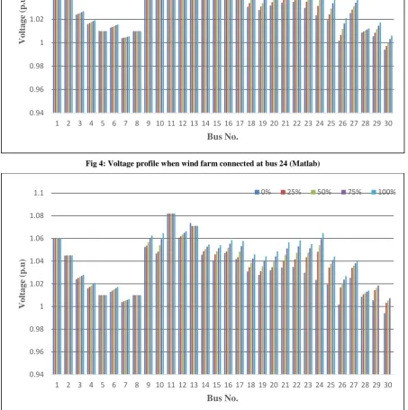
The wind farm is connected at bus 10 and bus 24 (20 MW in each bus) separately, for penetration levels from 25% to 100% with an interval of 25%. From Table 3, it can be seen that the total generation cost, minimum voltage (level & phase angle) values, total active and active power generation, power flow of transmission lines, the active and reactive power losses (Table 3) , and Fig.3 and 4 shows the voltage profiles.

7.3

Impact of Multiple Wind Farm

In this case we show the impact of integration wind farm connected to bus 10 and bus 24 (20 MW in each bus) together. For penetration levels from 25% to 100% with an interval of 25%. From table 3, it can be seen that the total generation cost, minimum voltage (level & phase angle) values, total active and active power generation, power flow of transmission lines, the active and reactive power losses, and Fig. 5 shows the voltage profiles.

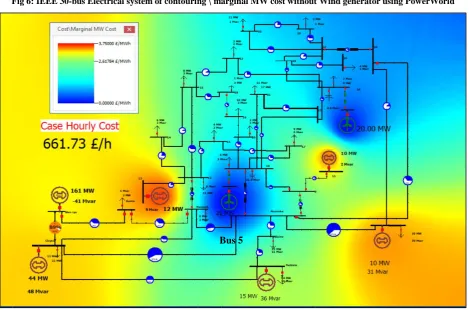
From table 3 (Wind farm connected to bus 10 & 24), the results show that variable wind power reduces the cost generation level, by optimal power flow. When system operate without wind farm show that the high MW cost of in generator at bus 5 at rated power 22MW as shown in Fig .6, but when integrated wind farm to bus 10 and 24 at fill rated power (20MW in each wind farm) effect to reduce MW generator at bus 5 to 15MW and reduce cost of it shown in Fig. 7. Thus, wind farms will be reduce the cost of fuel for conventional power plants.

Fig 2:IEEE 30-bus Electrical system with two Wind generator at bus10&bus 24

Table 3. Results of LPOPF when connected wind farm with different wind penetration levels

Wind farm connected at bus 10

Variable PowerWorld Matlab

Wind penetration 0% 25% 50% 75% 100% 0% 25% 50% 75% 100%

slack bus (MW) 178 191 185 180 175 176 175 171 166 160

Cost($hr) 803.91 785.4

6

766.73 748.5

3

730.4 2

802.46 791.03 776.83 764.63 753.42

Losses (MW) 10.54 10.58 10.09 9.63 9.20 10.31 9.12 9.05 8.79 8.27

Losses (Mvar) 20.23 19.18 19.08 18.94 18.9 19.67 19.12 18.74 18.15 17.8

Vmin (p.u.) 0.9937 0.994

5

0.9953 0.996

1

0.996 8

0.9953 0.9964 0.9975 0.9986 0.9993

Min angle (°) -13.84 -13.55 -13.27 -12.98 -12.69 -13.42 -13.04 -12.89 -12.78 -12.62

Line flow 1-2 (MVA %)

106 103 103 102 101 95 93 90 88 87

Wind farm connected at bus 24

Variable PowerWorld Matlab

Wind penetration 0% 25% 50% 75% 100% 0% 25% 50% 75% 100%

WF at Bus 24

Slack bus (MW) 178 191 185 180 174 176 177 172 168 163

Cost($hr) 803.91 784.9

6

766.14 747.6

6

729.7 2

802.46 790.89 776. 764.63 753.42

Losses (MW) 10.54 10.45 9.89 9.39 8.95 10.31 9.03 8.85 8.34 7.96

Losses (Mvar) 20.23 20.05 19.83 19.71 19.58 19.67 19.03 18.61 18.11 17.83

Vmin (p.u.) 0.9937 0.997

2

1.0003 1.003

2

1.006 1

0.9953 0.9985 1.0014 1.0046 1.0061

Min angle (°) -13.84 -13.44 -13.03 -12.64 -12.24 -13.42 -12.93 -12.74 -12.61 -12.5

Line flow 1-2 (MVA %)

106 103 102 102 101 95 93 89 88 87

Wind farm connected at bus 10 & 24

Variable PowerWorld Matlab

Wind penetration 0% 25% 50% 75% 100% 0% 25% 50% 75% 100%

Slack bus (MW) 178 185 174 170 161 176 170 159 148 138

Cost($hr) 803.91 766.0

3

729.58 695.6

5

661.7 3

802.46 758.89 736.91 701.78 680.59

Losses (MW) 10.54 9.85 8.94 8.76 8.15 10.31 9.03 8.85 8.34 7.96

Losses (Mvar) 20.23 19.1 18.05 17.73 17.13 19.67 18.81 18.47 18.0 17.63

Vmin (p.u.) 0.9937 1.003

2

1.00572 1.008 9

1.019 3

0.9953 1.00745 1.00937 1.01528 1.01694

Min angle (°) -13.84 -13.4 -13 -12.43 -12 -13.42 -12.81 -12.69 -12.6 -12.05

Line flow 1-2 (MVA %)

106 102 100 99 98 95 93 89 87 86

Fig 3: Voltage profile when wind farm connected at bus 10 (Matlab) 0.94

0.96 0.98 1 1.02 1.04 1.06 1.08 1.1

1 2 3 4 5 6 7 8 9 10 11 12 13 14 15 16 17 18 19 20 21 22 23 24 25 26 27 28 29 30

V

ol

tage

(p.u)

Bus No.

Fig 4: Voltage profile when wind farm connected at bus 24 (Matlab)

Fig5: Voltage profile when wind farm connected at bus 10 & 24 (Matlab) 0.94

0.96 0.98 1 1.02 1.04 1.06 1.08 1.1

1 2 3 4 5 6 7 8 9 10 11 12 13 14 15 16 17 18 19 20 21 22 23 24 25 26 27 28 29 30

Vo

lt

a

g

e

(p.u)

Bus No.

0% 25% 50% 75% 100%

0.94 0.96 0.98 1 1.02 1.04 1.06 1.08 1.1

1 2 3 4 5 6 7 8 9 10 11 12 13 14 15 16 17 18 19 20 21 22 23 24 25 26 27 28 29 30

Vo

lt

a

g

e

(p.u)

Bus No.

Fig 6: IEEE 30-bus Electrical system of contouring \ marginal MW cost without Wind generator using PowerWorld

Fig 7: IEEE 30-bus Electrical system of contouring \ marginal MW cost without Wind generator using PowerWorld

8.

CONCLUSION

This paper proposes the application of linear programming optimal power flow for a system that incorporates thermal units and wind farms during normal operation. The modified IEEE 30 system with six thermal generating units and two wind farms is used to analyse the impact of connected wind farm on the total generation cost, voltage profile, the power

power losses, by optimally integrate the wind farm in power systems. Based on the technical results it has been concluded that an optimal integration, location and utilization of wind farms give significant benefit example like such as reducing in the fuel cost, real and active power losses, the power flow of transmission lines loaded with more than the allowable limit and amelioration in the voltage profile. The results obtained

Bus 5

power losses and voltage profile. Finally, the results are very much promising.

9.

REFERENCES

[1] Reid Dorsey-Palmateer. 2019. “Effects of wind power intermittency on generation and emissions,” The Electricity Journal, vol. 32, no. 3, pp. 25–30.

[2] Global Wind Energy Council (GWEC). April 2019. “Global wind report: Annual market update,” 2018, available at: http://www.gwec.net, accessed on.

[3] C. Shilaja and T. Arunprasath. 2019. “Optimal power flow using Moth Swarm Algorithm with Gravitational Search Algorithm considering wind power,” Future Generation Computer Systems, vol. 98, pp. 708–715.

[4] Partha P. Biswas, P.N. Suganthan. and Gehan A.J. Amaratunga.2017. “Optimal power flow solutions incorporating stochastic wind and solar power,” Energy Conversion and Management, vol. 148, pp. 1194–1207.

[5] H.R.E.H. Bouchekara, A.E. Chaib, M.A. Abido and R.A.El-Sehiemy.2016. “Optimal power flow using an improved colliding bodies optimization algorithm,” Applied Soft Computing, vol. 42, pp.119–131

[6] Firas Mohammed Tuaimah, Yaser Nadhum Abd and Fahad A. Hameed. 2013. “Ant Colony Optimization based Optimal Power Flow Analysis for the Iraqi Super High Voltage Grid,” International Journal of Computer Applications, vol. 67, no. 11, pp. 13–18.

[7] Khaled Zehar and Samir Sayah.2008. “Optimal power flow with environmental constraint using a fast successive linear programming algorithm: Application to the algerian power system,” Energy Conversion and Management, vol. 49, no. 11, pp. 3362–3366.

[8] Yun-Su Kim.2019. “A voltage deviation-memorizing reactive power controller for renewable energy sources,” Electrical Power and Energy Systems, vol. 107, p. 47–57

[9] Mengxia Wang, Ming Yang, and X. Han. 2020. “Optimal power flow considering transient thermal behavior of overhead transmission lines,” Electrical Power and Energy Systems., vol. 114, p. 105396.

[10] Serhat Duman , UğurGüvenç , Yusuf Sönmez, and Nuran Yörükeren. 2012. “Optimal power flow using gravitational search algorithm,” Energy Convers. Manag, vol. 59, pp. 86–95.

[11] Sadjad Galvani and Saeed Rezaeian Marjani. 2019. “Optimal power flow considering predictability of power systems,” Electric Power Systems Research, vol. 171, pp. 66–73.

[12] Khamees, Amr Khaled, N. M. Badra, and Almoataz Y. Abdelaziz.2016. “Optimal Power Flow Methods : A Comprehensive Survey,” International Electrical Engineering Journal (IEEJ), vol. 7, no. 4, pp. 2228–2239.