Exponential Spline Solution for Singularly Perturbed Boundary Value Problems with an Uncertain—But—Bounded Parameter

(1)

http://www.scirp.org/journal/jamp ISSN Online: 2327-4379

ISSN Print: 2327-4352

DOI: 10.4236/jamp.2018.64073 Apr. 25, 2018 854 Journal of Applied Mathematics and Physics

Exponential Spline Solution for Singularly

Perturbed Boundary Value Problems with

an Uncertain—But—Bounded Parameter

W. K. Zahra

1,2

, M. A. El-Beltagy

3

, A. M. El Mhlawy

1

, R. R. Elkhadrawy

1

1_{Department of Physics and Engineering Mathematics, Faculty of Engineering, Tanta University, Tanta, Egypt}

2_{Department of Mathematics, Basic and Applied Sciences Institute, Egypt-Japan University of Science and Technology,} Alexandria, Egypt

3_{Department of Engineering Mathematics and Physics, Faculty of Engineering, Cairo University, Giza, Egypt}

Abstract

In this paper, we develop a new numerical method which is based on an ex-ponential spline and Shishkin mesh discretization to solve singularly per-turbed boundary value problems, which contain a small uncertain perturba-tion parameter. The proposed method uses interval analysis principle to deal with the uncertain parameter and the Monte Carlo Simulations (MCS) are used to validate the solution and the accuracy of the proposed method. Fur-thermore, sensitivity analysis has been conducted using different methods to assess how much the solution is sensitive to the changes of the perturbation parameter. Numerical results are provided to show the applicability and effi-ciency of the proposed method, which is ε-uniform convergence of almost second order.

Keywords

Singular Perturbation Problem, Shishkin Mesh, Two Small Parameters, Exponential Spline, Interval Analysis, Sensitivity Analysis, Monte Carlo Simulations

1. Introduction

In this paper, we consider the following singularly perturbed problem [1];

( )

,

[ ]

,

y′′ µf x y′ g x y r x x a b

− + + = ∈ (1) subject to the following boundary conditions,

How to cite this paper: Zahra, W.K., El-Beltagy, M.A., El Mhlawy, A.M. and Elk-hadrawy, R.R. (2018) Exponential Spline Solution for Singularly Perturbed Boundary Value Problems with an Uncertain—But— Bounded Parameter. Journal of Applied Ma-thematics and Physics, 6, 854-863.

https://doi.org/10.4236/jamp.2018.64073

Received: March 21, 2018 Accepted: April 22, 2018 Published: April 25, 2018

(2)

DOI: 10.4236/jamp.2018.64073 855 Journal of Applied Mathematics and Physics

( )

0

y a − =α y b − =β (2)

where 0<1 and 0<µ1 are two small perturbation parameters;

( ) ( )

,

f x g x and r x

( )

are sufficiently smooth functions for x∈

[ ]

a b, ; a, b, α,

and β are real constants. In general, the solution y x

( )

may exhibit two

boundary layers of exponential type at both end points x=a b, .

Different applications in science and engineering consider these kinds of problems that describe complicated physical and chemical models such as heat transfer problems, Navier-Stokes flow with large Reynolds numbers, chemical reactor theory, convection-diffusion processes, geophysics, aerodynamics, reac-tion-diffusion processes, quantum mechanics and optimal control, etc. Its solu-tion exhibits two layers at the two endpoints of the domain. The nature of the two-parameter problem was asymptotically examined by [2]. It was found that layer-adapted meshes have been required to obtain a uniformly convergent method no matter how small the perturbation parameter see [3] for more details.

Many numerical methods have been developed for the solution of two layer boundary value problems, such as described in [4], [5], [6] and [7] for one rameter singularly perturbed boundary value problems and with two small pa-rameters are considered in [1], [3], [8] and [9], but on a Shishkin-type mesh. Vulanovic [10] considered Shishkin and Bakhvalov meshes but assumed

1 2

p

µ= + with p > 0. Dag and Sahin presented a numerical solution of singularly perturbed boundary value problems, using finite element method [11]. Their collocation method was applied with quadratic and cubic B-spline base functions over the geometrically graded mesh of the solution domain. In 2010, Rashidina and Mohammadi [12] considered the self-adjoint singularly perturbed two-point boundary value problems. Ramadan et al. (2007) [13] developed quintic non-polynomial spline methods for the numerical solution of fourth order two-point boundary value problems. A second order monotone numerical method was constructed by Gracia et al. in 2006 [14] for a singularly perturbed ordinary dif-ferential equation with two small parameters affecting the convection and diffu-sion terms. The monotone operator was combined with a piecewise uniform Shishkin mesh. Kadalbajoo and Yadaw [15] presented a B-spline collocation method for solving a class of two-parameter singularly perturbed boundary value problems. They used B-spline collocation method on piecewise-uniform Shishkin mesh, which leads to a tridiagonal linear system. Their method was shown to have a uniform convergence of second order.

(3)

the random parameter, then a unique solution is defined by carrying out the de-terministic solver for each of these realizations. In 1967, Stein [18] generalized his model which incorporates stochastic effects due to neuronal excitations to handle a distribution of post-synaptic potential amplitudes and used the Monte-Carlo technique for approximating the solution. David Edwards [19] de-veloped a multi-region FDM technique for a particular singularly perturbed boundary value problem and this method was based on Monte Carlo tech-niques.

The main contribution of this paper is to develop a new spline method based on a Shishkin mesh discretization for obtaining an approximation for the solu-tion of two-layer boundary value problems. As the perturbasolu-tion parameter is not deterministic, therefore the interval analysis is considered to estimate the solu-tion range. The validasolu-tion of the developed solver will be done by comparing the exact and the approximate solutions of the proposed method and the MCS re-sults. The convergence analysis also is presented numerically and shows that the presented method is almost second-order.

The paper is organized as follows: In Section 2, we derive our spline scheme. Mesh strategy based on a Shishkin mesh is presented in Section 3. In Section 4, we present interval analysis and sensitivity measures. Numerical results are dis-cussed in Section 5. Section 6 is devoted to the final conclusions, while future work is provided in section 7. Finally, Section 8 is dedicated to references.

2. Derivation of Exponential Spline

We discretize the solution region Ω =

[ ]

a b, such that

0 1 2 N 1 N

a=x < <x x <<x ₋ <x =b. Where N is the number of mesh points. Let

1 , 1, 2,3, ,

j j j

h =x+ −x j=  N be the mesh size and the mesh ratio

1

0, 1, 2, 3, , 1

j j

j

h

j N

h

σ ₌ + _> ₌ ₋

 . When

σ

=1 the mesh reduces to a uniform

mesh, hj+1=hj=h. The interpolating exponential spline approximation

func-tion can be defined as [20]:

( )

_j _j

(

_j

)

_j _j j _j _j j , 0,1, , 1

j j

x x x x

S x a b x x c d j N

h h

ξ  −  ζ  − 

= + − + _ _+ _ _ = −

     (3)

where

( )

2

( )

2 cosh 1

j x x

ξ

=

τ

_

τ

− _ _, 3

( )

6 sinh

j x x

ζ

=

τ

_

τ

−

τ

_ _, a b c d_j, _j, _j, _j

are constants and τ is a free parameter such that the non-polynomial spline (3) reduces to usual cubic spline when τ approaches to zero [21], which satisfies the following conditions:

1)

( )

2

[ ]

,

j

S x ∈C a b ,

2) S x

( ) ( ) ( )

j =y xj ,S′′ xj =Mj. (4)

The algebraic manipulations of Equations (3) and (4) yield the following ex-pressions:

(4)

2)

(

1

)

2 1 2

1

coth sinh

j j j j

j j j j j

j

h h h h

b y y M M

h + τ τ τ + τ τ τ

   

= − +_ − _ +_ − _

    ,

3) 2

2

j

j j

h

c = M ,

4)

(

)

2

1 cosh

6 sinh

j

j j j

h

d τ M M τ

τ +

= − _{. (5)}

From the aspect of the first derivative continuity at the mesh points yields the expression for the determination of S′′

( )

xj where i=0,,N. We can get the

following exponential spline identity relation:

(

)

(

)

1 1 1 1 1 1 1

j j j j j j j j j j j j j j

y₊ − +σ y +σ y₋ =h h₋ _α M ₊ + +σ β M +γ M ₋_ (6)

where

(

)

2

coth

1 1 1

, ,

sinh

1 1

sinh coth cosh , 1, 2,

j

j j

j j j j

j

j j j j

j j

j

τ

α β

τ τ τ τ

τ

γ τ τ τ

τ τ

= − = −

= + − = _

(7)

Note that, the exponential spline relation (6) is consistent with the standard variable-mesh cubic spline if

τ

→0 , hence 1, 1

6 3

α γ= = β = _[22]_{. If we}

choose 1, 5

12 12

α γ= = β = _{, this method is known as the Numerov method}_[23]_.

3. Mesh Selection Strategy

We consider the simplest possible non-uniform mesh, namely a piecewise-uniform mesh proposed by Shishkin [24]. The domain is Ω =

[ ]

a b, into three

sub-domains

[

, 1

]

,

[

1, 2

]

,

[

2,

]

l a a ω c a ω b ω r b ω b

Ω = + Ω = + − Ω = −

where the transition parameters are given by:

[ ]

( )

[ ]

( )

1 2

1 , 1 2 , 2

1 2 1 2

min , ln , min , ln

4 4

and max_{x a b} , min_{x a b}

N N

x x

ω ω

ϕ ϕ

ϕ _∈ λ ϕ _∈ λ

   

= _ _ = _ _

   

= − =

(8)

where λ1

( )

x and λ2

( )

x are two solutions of the characteristic equation:

( )

( ) ( )

( )

2 _x _{f x} _x _{g x} ₀

λ µ λ

− + + = (9) The quantity λ <1 0 describes the boundary layer at x=a, while λ >2 0

characterizes the layer at x=b, and

[ ]

( )

2 2 2 2

1 2 ,

4 4

, , where max

2 2 x a b

B B C B B C

B f x

µ µ µ µ

λ = − +  λ = + +  = _∈

  (1

0) We take N/4, N/2 and N/4 mesh points, respectively in Ω Ωl, c and Ωr.

De-note the step sizes in each subinterval byh1=4ω1 N, h2=2

(

b− −a ω ω1− 2

)

N

(5)

Shishkin mesh is represented by:

(

)

1

1 1 1

1 2

2 1 1

2

3 1 1

4

; for 1, 2, , 4 ,

2

; for 1, , 3 4 ,

4

4 3

; for , , .

4

j j

h x x h j N

N

b a N

h h x x h j N

N

h x x h j N

N ω ω ω ω ∨ − − −  = = + =   − − −  = = = + = +   = = + =      (11)

4. Interval and Sensitivity Analysis

Since uncertainty will be considered, the interval analysis can be used as descrip-tive measures of uncertainty in quantitadescrip-tive values. Hence, the perturbation pa-rameter is not deterministic, the solution has to be defined as a range based on the interval of the parameter. Therefore, the upper and lower bounds of the per-turbation parameter can be written as:

,

c c

= + ∆ = − ∆

      (12)

where  is the upper value,  is the lower value and _c is the central value.

Then the fluctuation range of solution could be estimated.

Sensitivity measures can be conducted using different techniques for example One-at-a-Time Sensitivity Measures (±SD), the Sensitivity Index (SI), the Im-portance Index (II), Differential Sensitivity Analysis (PD), etc. We estimated the sensitivity measures using the following methods One-at-a-Time Sensitivity Measures (±SD), the Sensitivity Index, and the Differential Sensitivity Analysis. One-at-a-Time Sensitivity Measures (±SD) is considered the simplest—but pow-erful—method for conducting sensitivity analysis, which estimates the variation of the solution as the perturbation parameter is increased by a factor of its standard deviation or in other words a percentage of its mean value [25].

The Sensitivity Index (SI), another simple method of estimating the sensitivity measure is to calculate the relative solution difference when varying one input parameter from its minimum value to its maximum value, which provides a good indication of parameter and model variability. The SI is calculated using,

(

)

SI= Ymax−Ymin Ymax, where Ymin and Ymax represent the minimum

and maximum solution values, respectively, resulting from varying the perturba-tion parameter over its entire range [26].

Differential Sensitivity Analysis (PD) method considers all random parame-ters equal to their mean values and partial differentiation of the system with re-spect to the random parameters should be done. The sensitivity coefficient for a specific parameter –perturbation parameter can be measured from the partial derivative relation∂ ∂y . The results are normalized by multiplying the

deriva-tives by the ratio of the parameter value to the solution for the mean value, sen-sitivity coefficient = ∂ ∂ ∗y 

(

 y

)

[25].

5. Numerical Example

(6)

[ ] ( )

( )

cosπ , 0,1 , 0 1 0

y′′ y x x y y

− + = ∈ = = (13) whose exact solution is given by:

( )

2 1

2 2

1 2 1 2 1

1 2 3

1 2 2 1 3 1 1,2

cosπ e e

1 1 e 1 e 1

, , ,

π 1 1 e 1 e

x x

Y c x c c

c c c c c

λ λ

λ λ λ λ λ

− −

−

− −

= + +

+ +

= = − = =

+ − − 

 

(14)

The estimated maximum error EN and the rate of convergence rN are

computed by the formulas:

0 2 2 2

max , log log

N j N j j N N N

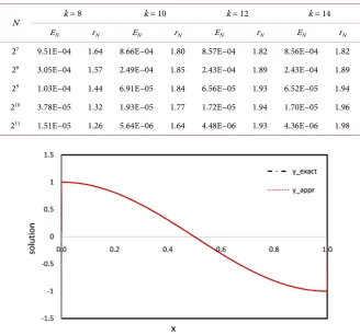
[image:6.595.206.541.75.222.2] [image:6.595.208.537.395.701.2]

E = _{< <} Y −y r = E − E (15)

Table 1 shows the maximum absolute error and the order of convergence for various values of the perturbation parameter ℇ. The results obtained using the current method are very accurate compared with the analytical solution and gives the order of convergence 2 even for small values of ℇ, and it is shown in

Figure 1 that the exact and the approximate solutions are very close. Further-more, since the problem is singularly perturbed its solution possesses layers along the boundary of the domain which is occurred in the form of sharp boun-dary-layers in Figure 1 at x=0,1.

Figures 2-4 show the comparison of the solution between the proposed method and the MCS (50000 samples), as the perturbation parameter changes by 20%.

Table 1. Maximum absolute errors and the order of convergence for _=10−k.

N k = 8 k = 10 k = 12 k = 14

EN rN EN rN EN rN EN rN

27 _9.51E−04 _1.64 _8.66E−04 _1.80 _8.57E−04 _1.82 _8.56E−04 _1.82

28 _3.05E−04 _1.57 _2.49E−04 _1.85 _2.43E−04 _1.89 _2.43E−04 _1.89

29 _1.03E−04 _1.44 _6.91E−05 _1.84 _6.56E−05 _1.93 _6.52E−05 _1.94

210 _3.78E−05 _1.32 _1.93E−05 _1.77 _1.72E−05 _1.94 _1.70E−05 _1.96

211 _1.51E−05 _1.26 _5.64E−06 _1.64 _4.48E−06 _1.93 _4.36E−06 _1.98

Figure 1. Deterministic Case: exact and approximate solutions for 14

10− =

(7)

[image:7.595.230.517.73.242.2]

DOI: 10.4236/jamp.2018.64073 860 Journal of Applied Mathematics and Physics Figure 2. Random Case: Mean of the solution of the proposed method and the MCS results, _=₁₀−14, _N=₂₅₆.

Figure 3. Random Case: Upper limit of the solution range of the proposed method and the MCS results, 14

10− =

 , N=256.

Figure 4. Random Case: limit of the solution range of the proposed method and the MCS results, 14

10− =

[image:7.595.230.517.296.470.2] [image:7.595.231.517.518.692.2]

(8)

The upper, centre and lower solutions of the two methods are very close which shows the accuracy and validation of the proposed method. Further sensitivity measures have been conducted such as the SI method gives an index of value 0.0039%, which is very small. The differential method indicates that the sensitiv-ity coefficient is also very small by value 1.34E−15 at the mid-point of the scheme. Therefore, the solution is not sensitive to the changes in the perturba-tion parameter.

6. Conclusion

A numerical method based on exponential spline with Shishkin mesh discretiza-tion is combined with interval analysis perspective to evaluate the range of the solution for the singularly perturbed two-point boundary value problems with uncertain parameter. The numerical results show that the present method ap-proximates the solution very well compared with the exact solution. Therefore, the proposed method is almost second-order uniformly convergent with respect to the perturbation parameter. MCS are used to prove the validation and the ac-curacy of the proposed method. Sensitivity analysis has been conducted using different methods and it is found that the solution is not sensitive to the pertur-bation parameter.

7. Future Work

This paper proposed a new numerical spline method combined with interval analysis to solve singularly perturbed boundary value problems. We used inter-val analysis to estimate the solution range as the perturbation parameter is not deterministic and compared the results with the MCS method to validate the proposed method. In the future, we shall use another stochastic method to deal with the uncertainty, which appears in the perturbation parameter for example polynomial chaos expansion.

References

[1] Zahra, W.K. and Van Daele, M. (2015) Uniformly Convergent Discrete Spline Scheme on a Shishkin Mesh for the Singular Perturbation Boundary Value Problem.

Proceedings of the 15th International Conference on Mathematical Methods in Science and Engineering, CMMSE 2015,6-10 July 2015, Cádiz, 1261-1268.

[2] O’Malley, R.E. (1967) Singular Perturbations of Boundary Value Problems for Lin-ear Ordinary Differential Equations Involving Two Parameters. Journal of Mathe-matical Analysis and Applications, 19, 291-308.

https://doi.org/10.1016/0022-247X(67)90124-2

[3] Zahra, W.K. and Van Daele, M. (2018) Discrete Spline Solution of Singularly Per-turbed Problem with Two Small Parameters on a Shishkin-Type Mesh. Computa-tional Mathematics and Modeling Journal. (To be published)

(9)

DOI: 10.4236/jamp.2018.64073 862 Journal of Applied Mathematics and Physics [5] Duvnjaković, E., Karasuljić, S., Pasic, V. and Zarin, H. (2014) A Uniformly Conver-gent Difference Scheme on a Modified Shishkin Mesh for the Singular Perturbation Boundary Value Problem.arXiv Prepr. arXiv1411.4323

[6] Ramadan, M.A., Lashien, I.F. and Zahra, W.K. (2007) The Numerical Solution of Singularly Perturbed Boundary Value Problems Using Nonpolynomial Spline. In-ternational Journal of Pure and Applied Mathematics, 41, 883-896.

[7] Zahra, W.K., El-Azab, M.S. and El Mhlawy, A.M. (2014) Spline Difference Scheme for Two-Parameter Singularly Perturbed Partial Differential Equations. Journal of Applied Mathematics & Informatics, 32, 185-201.

https://doi.org/10.14317/jami.2014.185

[8] Natesan, S., Gracia, J.L. and Clavero, C. (2004) Singularly Perturbed Bound-ary-Value Problems with Two Small Parameters: A Defect Correction Approach.

Proceedings of the International Conference on Boundary and Interior Layers,

Computational and Asymptotic Methods, BAIL, Bail, 1-6. https://www.springer.com/br/book/9783319257259

[9] Kumar, M. and Rao, S.C.S. (2010) High Order Parameter-Robust Numerical Method for Singularly Perturbed Reaction-Diffusion Problems. Applied Mathemat-ics and Computation, 216, 1036-1046. https://doi.org/10.1016/j.amc.2010.01.121 [10] Vulanović, R. (2001) A Higher-Order Scheme for Quasilinear Boundary Value

Problems with Two Small Parameters. Computing, 67, 287-303. https://doi.org/10.1007/s006070170002

[11] Dag, I. and Sahin, A. (2009) Numerical Solution of Singularly Perturbed Problems.

The International Journal of Nonlinear Science, 8, 32-39. http://www.internonlinearscience.org/

[12] Rashidinia, J. and Mohammadi, R. (2010) Non-Polynomial Spline Approximations for the Solution of Singularlyperturbed Boundary Value Problems. TWMS Journal of Pure and Applied Mathematics, 1, 236-251.

http://www.naturalspublishing.com/show.asp?JorID=53&pgid=0

[13] Ramadan, M.A., Lashien, I.F. and Zahra, W.K. (2009) Quintic Nonpolynomial Spline Solutions for Fourth Order Two-Point Boundary Value Problem. Commu-nications in Nonlinear Science and Numerical Simulation, 14, 1105-1114. https://doi.org/10.1016/j.cnsns.2007.12.008

[14] Gracia, J.L., O’Riordan, E. and Pickett, M.L. (2006) A Parameter Robust Second Order Numerical Method for a Singularly Perturbed Two-Parameter Problem. Ap-plied Numerical Mathematics, 56, 962-980.

https://doi.org/10.1016/j.apnum.2005.08.002

[15] Kadalbajoo, M.K. and Yadaw, A.S. (2008) B-Spline Collocation Method for a Two-Parameter Singularly Perturbed Convection-Diffusion Boundary Value Prob-lems. Applied Mathematics and Computation, 201, 504-513.

https://doi.org/10.1016/j.amc.2007.12.038

[16] Moore, R.E. (1966) Interval Analysis. Prentice-Hall, Englewood Cliff, NJ.

[17] Le Maitre, O. and Knio, O.M. (2010) Spectral Methods for Uncertainty Quantifica-tion: With Applications to Computational Fluid Dynamics. Springer Science & Business Media, New York.

[18] Stein, R.B. (1967) Some Models of Neuronal Variability. Biophysical Journal, 7, 37-68. https://doi.org/10.1016/S0006-3495(67)86574-3

(10)

DOI: 10.4236/jamp.2018.64073 863 Journal of Applied Mathematics and Physics Kong, 18-20 March 2009.

[20] Zahra, W.K. (2011) Finite-Difference Technique Based on Exponential Splines for the Solution of Obstacle Problems. International Journal of Computer Mathematics, 88, 3046-3060. https://doi.org/10.1080/00207160.2011.573846

[21] Tirmizi, I.A., Fazal-i-Haq and Siraj-ul-Islam (2008) Non-Polynomial Spline Solu-tion of Singularly Perturbed Boundary-Value Problems. Applied Mathematics and Computation, 196, 6-16. https://doi.org/10.1016/j.amc.2007.05.029

[22] Mohanty, R.K., Nayak, S. and Khan, A. (2017) Non-Polynomial Cubic Spline Dis-cretization for System of Non-Linear Singular Boundary Value Problems Using Variable Mesh. Advances in Difference Equations, 2017, 327.

[23] Henrici, P. (1962) Discrete Variable Methods in Ordinary Differential Equations.

ZAMM-Journal of Applied Mathematics and Mechanics/Zeitschriftfür Angewandte Mathematik und Mechanik. https://onlinelibrary.wiley.com/journal/15214001 [24] Shishkin, G.I. (1988) Grid Approximation of Singularly Perturbed Parabolic

Equa-tions with Internal Layers. Russian Journal of Numerical Analysis and Mathemati-cal Modelling, 3, 393-408. https://doi.org/10.1515/rnam.1988.3.5.393

[25] Hamby, D.M. (1994) A Review of Techniques for Parameter Sensitivity Analysis of Environmental Models. Environmental Monitoring and Assessment, 32, 135-154. https://doi.org/10.1007/BF00547132

[26] Hoffman, F.O. and Miller, C.W. (1983) Uncertainties in Environmental Radiologi-cal Assessment Models and Their Implications. Annual Meeting of the National Council of Radiation Protection and Measurements, Washington DC, 6 April 1983. [27] Khan, A. and Khandelwal, P. (2014) Non-Polynomial Sextic Spline Solution of

Sin-gularly Perturbed Boundary-Value Problems. International Journal of Computer Mathematics, 91, 1122-1135. https://doi.org/10.1080/00207160.2013.828865

[28] Zahra, W.K. and El Mhlawy, A.M. (2013) Numerical Solution of Two-Parameter Singularly Perturbed Boundary Value Problems via Exponential Spline. Journal of King Saud University-Science, 25, 201-208.