www.hydrol-earth-syst-sci.net/14/279/2010/ © Author(s) 2010. This work is distributed under the Creative Commons Attribution 3.0 License.
Earth System
Sciences
Implementing small scale processes at the soil-plant interface – the
role of root architectures for calculating root water uptake profiles
C. L. Schneider1, S. Attinger1,2, J.-O. Delfs3, and A. Hildebrandt1
1Helmholtz Centre for Environmental Research – UFZ, Department of Computational Hydrosystems, Leipzig, Germany 2Institute for Geosciences, University of Jena, Jena, Germany
3Helmholtz Centre for Environmental Research – UFZ, Department of Environmental Informatics, Leipzig, Germany Received: 19 May 2009 – Published in Hydrol. Earth Syst. Sci. Discuss.: 12 June 2009
Revised: 20 January 2010 – Accepted: 24 January 2010 – Published: 12 February 2010
Abstract. In this paper, we present a stand alone root water uptake model called aRoot, which calculates the sink term for any bulk soil water flow model taking into account wa-ter flow within and around a root network. The boundary conditions for the model are the atmospheric water demand and the bulk soil water content. The variable determining the plant regulation for water uptake is the soil water potential at the soil-root interface. In the current version, we present an implementation of aRoot coupled to a 3-D Richards model. The coupled model is applied to investigate the role of root architecture on the spatial distribution of root water uptake. For this, we modeled root water uptake for an ensemble (50 realizations) of root systems generated for the same species (one month old Sorghum). The investigation was divided into two Scenarios for aRoot, one with comparatively high (A) and one with low (B) root radial resistance. We com-pared the results of both aRoot Scenarios with root water up-take calculated using the traditional Feddes model. The ver-tical rooting density profiles of the generated root systems were similar. In contrast the vertical water uptake profiles differed considerably between individuals, and more so for Scenario B than A. Also, limitation of water uptake occurred at different bulk soil moisture for different modeled individu-als, in particular for Scenario A. Moreover, the aRoot model simulations show a redistribution of water uptake from more densely to less densely rooted layers with time. This behav-ior is in agreement with observation, but was not reproduced by the Feddes model.
Correspondence to: C. L. Schneider ([email protected])
1 Introduction
The global water and carbon cycles are key issues in climate and global change research. Within these complex systems, plants are the central interface between the atmosphere and hydrosphere. Transpiration plays a crucial role for the sur-face energy balance as well as for the water cycle. It is also linked to the carbon cycle through its close connection with photosynthesis. Hydrological as well as climate mod-els will benefit from an improved understanding of the pro-cess of water flow through plants, in particular because they are sensitive to root water uptake parameters (Desborough, 1997; Zeng et al., 1998). Also, great uncertainty in modeling transpiration stems from lack of knowledge about how much water is available to plant roots (Lai and Katul, 2000; Feddes et al., 2001).
Plant water uptake responds to soil moisture limitation at different time and space scales. At the seasonal time scale, plants may adapt their rooting system by root growth, in or-der to reach moister soil areas (Wan et al., 2002). But also at smaller time scales (like hours to days), plants have been observed to change their uptake zone, and without altering their root system (Sharp and Davies, 1985; Green and Cloth-ier, 1995; Garrigues et al., 2006).
In order to deal with these shortcomings, several algo-rithms have been developed to allow for a longer period of transpiration in a SVAT context. Li et al. (2001) and Teuling et al. (2006) presented models that compensate water stress in one part of the root zone by increased uptake from other soil areas without altering rooting density profiles. ˇSim˚unek and Hopmans (2009) followed a similar approach. They pro-posed a root water uptake compensation mechanism for HY-DRUS ( ˇSim˚unek et al., 2006, 2008), which allows for paral-lel consideration of compensated water and nutrient uptake in three dimensions. Also, besides compensation effects, an-other mechanism sustaining transpiration in dry soil, is hy-draulic redistribution. It is defined as water transfer from wetter into drier soil areas, via flow through the root sys-tem. Recently, Siqueira et al. (2008) and Amenu and Ku-mar (2008) investigated this effect for delayed onset of water stress in a root water uptake model, again based on rooting density profiles.
The above models treat uptake and adaptation in a lumped way, and therefore do not consider the mechanisms at the scale at which they take place. Models which include more detail could be used to gain the necessary process under-standing, in order to transfer it to the SVAT scale. Small scale processes of root water uptake have already been im-plemented in models of varying levels of complexity.
First level models distribute the transpirational demand on the soil domain simply by the spatial distribution of roots either in one (as SVAT models do), two or three dimensions (Vrugt et al., 2001; Clausnitzer and Hopmans, 1994).
Second level models include a description of microscopic water flow along the potential gradient between the soil and the root, either using an effective resistance along this gradi-ent like Gardner (1960, 1964) or more realistic radial depen-dent soil hydraulic properties (Tuzet et al., 2003; de Jong van Lier et al., 2006). The latter cover the nonlinear behavior of unsaturated water flow. This is an important mechanism in drying soils (Schr¨oder et al., 2008), because steep potential gradients develop around the roots. These models can be ex-tended to include root radial resistance additionally to soil resistance (Siqueira et al., 2008; Schymanski et al., 2008). For example Levin et al. (2007) showed with such a com-bined model that vertical uptake profiles changed depending on the assumed radial resistance. Schymanski et al. (2008) applied such a model to modify root distribution within bio-logical constraints according to soil water availability.
The approaches above imply that the potential on the side of the root is constant throughout the root system. However, Zwieniecki et al. (2003) suggested in a combined measure-ment and model study that internal gradients along the root xylem exist. Depending on the ratio between the roots radial and axial resistance, the active uptake region could extend over the entire root or just part of it. This research was con-ducted only for a single root, but might also be relevant for uptake along the entire root system.
Third level models combine a variable xylem potential dis-tribution along the root structure with the flow processes in the soil domain. One such model was introduced by Doussan et al. (1998). Such root water uptake models can be coupled to three dimensional soil water flow models as done in Dous-san et al. (2006) or Javaux et al. (2008). Simulations with these detailed models show that the region of water uptake moves with time to deeper and moister layers, when top lay-ers dry out. The coupling of soil and root water flow in the vicinity of the root segments was first based on an averaging approach. A finer spatial discretization of the numerical soil grid around the roots (as shown in Schr¨oder et al., 2009) can represent the local gradients in soil water potential but at the cost of increased computational burden.
In summary, previous research using small scale models for water uptake indicates that both water flow in the soil near the root, but also within the root system itself shape the uptake behavior of the plant. Plant root systems vary greatly in form and morphology, not only between species, but also between individuals of the same species. This chapter con-tributes to answer the question, how does this variety influ-ence the expected uptake pattern. Therefore, we propose a simplified third level model called aRoot and apply it to sim-ulate the water uptake of an ensemble of root systems of the same species and age. Our model results suggest that water uptake profiles vary significantly between individuals.
2 Models and methods
The major assumption for this study is that the process of plant water uptake is gradient driven by the difference be-tween soil water potential and atmospheric demand. In real plants, this leads to a distribution of water potentials from the leaves (stomata control) over the trunks to the stem and finally to the root system. Hence, the outer boundaries of the plants water uptake system are the atmospheric water deficit and the soil water potential. In this model exercise, we only consider the part from the soil up to the root collar. Within this study we make a comparison between two model ap-proaches for root water uptake. One approach uses a full 3-D Richards Equation (see Sect. 2.1) coupled to the Feddes reduction function (Sect. 2.4) to simulate soil water stress ef-fects on root water uptake. The other approach again uses the 3-D Richards Equation to model the bulk soil water flow combined with a smaller scale water uptake model called “aRoot” (Sect. 2.2). This “aRoot” model was divided into two scenarios of different root hydraulic parameterizations. 2.1 Bulk water flow in the unsaturated zone
The Richards’ equation describing the water movement in the soil system is known as
∂θ
where θ[m3m−3] is the volumetric soil water content, %[m3m−3s−1] is the sink term rate delivered by the root wa-ter uptake model (see Eq. 22) for the aRoot approach of vol-umetric flow rates) andt[s] is time. The numerical solution of the Richards Equation for bulk soil water flow is provided by GeoSys (Kolditz et al., 2008).
Volumetric soil water saturationθ is defined as a func-tion of the soil water potential ψsoil[m] and can be ex-pressed by the Mualem-van-Genuchten parametrization (van Genuchten, 1980) as
θ−θr φ−θr
=2=
1
1+ |αGψsoil|nG
mG
, (2)
where2is the normalized (or relative) water content, φis the porosity of the soil andθrthe residual volumetric water content (at so-called permanent wilting point), whereαG,nG andmGare soil specific parameters (see Table 1).K[m s−1] in terms of normalized (or relative) water content2is then given by
K(2)=Ksk(2)=Ks2λG
1−
1−2 1 mG
mG2
, (3)
where2can be replaced byψsoilusing Eq.(2). The saturated hydraulic conductivityKsas well as the bulk soil porosityφ are given in Table 1. Accounting for the effect of root seg-ments exploring a certain soil volume, within our model the porosity φ of all soil grid cells is decreased by the corre-sponding fraction of volumetric root content. This is moti-vated by the fact that as root volume increases in a certain soil volume, the soils pore space gets less and hence less wa-ter can be hold in this soil volume.
2.2 The hydraulic root water uptake model “aRoot” In the following, we present a stand alone root water uptake model called aRoot, which calculates the sink term for the bulk soil water flow model. Since we apply an analytical ex-pression for the radial water flow towards the root, our model concept does not require intense iteration between the bulk water flow model and aRoot for each time step.
2.2.1 Water flow within the root system
[image:3.595.307.550.96.439.2]Water flow within the plants takes place as a flow from root surface to the inner root xylem (radial) and along the xylem tubes (axial). The hydraulic uptake model applied to the root system is spatially explicit consisting of a network of root segments. Each individual root segment is modeled as a se-ries of axial and radial resistances similar to Doussan et al. (1998). These root resistances operate as an effective value for the underlying processes, like xylem development for the axial pathway and radial connectivity within the root cortex and epidermis (as described in Steudle and Peterson (1998) as the apoplastic, symplastic and transcellular pathways).
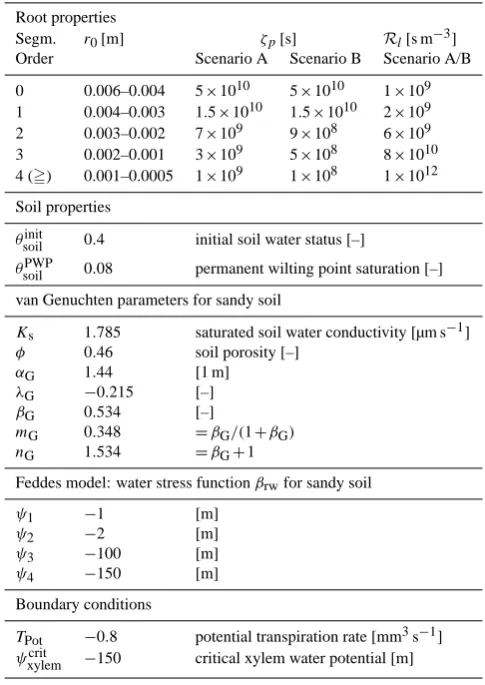
Table 1. Model parameters.
Root properties
Segm. r0[m] ζp[s] Rl[s m−3] Order Scenario A Scenario B Scenario A/B
0 0.006–0.004 5×10¹⁰ 5×10¹⁰ 1×10⁹ 1 0.004–0.003 1.5×10¹⁰ 1.5×10¹⁰ 2×10⁹ 2 0.003–0.002 7×10⁹ 9×10⁸ 6×10⁹ 3 0.002–0.001 3×10⁹ 5×10⁸ 8×10¹⁰ 4 (=) 0.001–0.0005 1×10⁹ 1×10⁸ 1×10¹²
Soil properties
θsoilinit 0.4 initial soil water status [–]
θsoilPWP 0.08 permanent wilting point saturation [–]
van Genuchten parameters for sandy soil
Ks 1.785 saturated soil water conductivity [µm s−1]
φ 0.46 soil porosity [–]
αG 1.44 [1 m]
λG −0.215 [–]
βG 0.534 [–]
mG 0.348 =βG/(1+βG)
nG 1.534 =βG+1
Feddes model: water stress functionβrwfor sandy soil
ψ1 −1 [m]
ψ2 −2 [m]
ψ3 −100 [m]
ψ4 −150 [m]
Boundary conditions
TPot −0.8 potential transpiration rate [mm3s−1]
ψxylemcrit −150 critical xylem water potential [m]
Root hydraulic properties are assigned to each root seg-ment according to their root order given by RootTyp (see Sect. 2.3 and Table 1). The axial resistanceRax is calcu-lated by multiplying the axial resistivity per length with the corresponding root lengthlr, while the radial resistanceRris estimated by dividing the specific radial resistivity (material property of each root segment) by root surface area.
The influence of osmotic potential differences are ne-glected as well as the effect of aquaporins changing the spe-cific radial resistivity per root segment (Steudle, 2000) or the effect of cavitation on xylem vulnerability increasing the ax-ial resistance (Sperry et al., 2003).
For each root segmentnthe axial flux is implemented by the formula
Jaxn = 1
Rn ax
1ψxylemn +1zn, (4)
from the soil to the root segmentnis given by
Jradn = 1
Rn r
(ψxylemn −ψsoiln (r0)) , (5)
withψxylemn denoting the xylem water potential within root segmentnandψsoiln (r0)the soil water potential at the root surface of the corresponding soil discn.
By applying the Kirchhoff’s Law for summing up all in-and outflows at a root node, we receive a system of equations describing the water fluxes of the root network that can be best described in matrix notation such as
Aψxylem=Bψsoil(r0)+c, (6)
where A is the system matrix (regarding radial and axial root resistances) coupling root xylem pressure for interlinked root nodes, B is the input matrix connecting xylem poten-tial to corresponding soil potenpoten-tials andcis the offset vec-tor accounting for gravitation (lifting water up over the ver-tical axis) and the upper boundary condition (flux or poten-tial boundary at root collar). The boundary condition at the root collar is initially fixed to a given fluxTPot. If the corre-sponding variable collar potential drops below a critical value
ψxylemcrit , then boundary switches to a potential condition and transpirational flux becomes variant.
Rearranging Eq. (6) gives
ψxylem=A−1Bψsoil(r0)+A−1c. (7) By rewriting Eq. (5) for all root segments N and in-troducing the conductance matrix κr (main diagonal ma-trix containing the inverse of the radial resistances κr= diag1/Rr0,...,1/Rrn,...,1/RrN) as well as new notations E=A−1B and d=A−1cleads to a system of equations for the overall radial fluxes in the root system, namely
Jrad=κr[(E−I)ψsoil(r0)+d], (8)
where I is the identity matrix of dimensionN, the overall number of root nodes. This system can be simplified to
Jrad=Wψsoil(r0)+ω , (9)
where W=κr(E−I)andω=κrd.
2.2.2 The microscopic radial water flow within the soil The microscopic flow towards the root is assumed to be only one dimensional in radial direction towards the root, where the soil domain is modeled as a cylinder of radiusrdisc and heightlr. Local hydraulic gradients in soil water potential
towards the root can be obtained with an approximated ana-lytical solution of the Richards equation (steady rate assump-tion after Jacobsen (1974) and De Willigen and van Noord-wijk (1987) where the temporal change in water content is assumed to berindependent)
∂θsoil
∂t =
1
r ∂ ∂r
K(ψsoil)r ∂ψsoil
∂r
=const. (10)
In matric flux potential notation, this equation becomes an ODE as
1
r ∂8soil
∂r +
∂28soil
∂r2 =const. , (11)
with the following solution
8soil(r)= τ3
4r 2+τ
2log(r)+τ1, (12)
where τp are integration constants set by boundary/initial
conditions.
The matric flux potential 8soil[m2s−1] is defined as a function of soil water potentialψsoilby
8soil(ψsoil)−8refsoil= ψsoil
Z
ψsoilref
K(h0soil)dh0soil, (13)
where8refsoil andψsoilref are reference states of the system. For
ψsoilref → −∞, the reference matric flux potential tends to
8refsoil→0, so
8soil(ψsoil)= ψsoil
Z
−∞
K(h0soil)dh0soil. (14)
The solution of this integral depends on the functional form of K(ψsoil). Unfortunately, for the Mualem-van-Genuchten parameterization used in our soil water model, no explicit solution is known. Therefore, a closed analytical relationship between water potentialhand matric flux poten-tial8cannot be established. Nevertheless, within a certain range ofh, the matric flux potential can be approximated by the following transfer function
8soil(r0)=b1exp
b2|ψsoil|b3+b4
, (15)
withbk soil dependent fitting parameters. For our
simula-tions, the soil parameters bk of Eq. (15) were fitted to the
numerical calculated8-h-profile for a sandy soil set up by the Mualem-van-Genuchten parameters given in Table 1.
The solution of Eq. 11 (similar to de Jong van Lier et al., 2008 or Schr¨oder et al., 2009) with given boundary condi-tions (zero flux at outer boundary, radial flux Jrad at inner boundary and a given bulk matric flux potential at a certain radial distancer8b) can be written as
8(r0)=8b+ Jrad 2π l
a2−γ+γlog(a2γ )
2−2γ
!
, (16)
Hence, the soil water flow corresponding to all root seg-ments is given by the gradient in matric flux potential be-tween the soil-root interface and the bulk soil multiplied with a function determined by the boundary conditions and hence depending on the segment geometry (given by Eq.16),
Jradn =gn 8nsoil(r0)−8nb
, (17)
with
gn= 4π l
n(1−γn)
a2−γn+γnlog(a2γn). (18)
Writing the radial soil water flow in matrix notation for all
Nsegments with G the main diagonal matrix containing the functional termsgn(G=diag
g0,..,gn,..,gN, we receive
Jrad=G(8soil(r0)−8b) . (19)
2.2.3 Coupling the root and radial soil water flow The radial root water flow (9) and the radial soil water flow (19) are set equal (coupled directly via flux type condition) Wψsoil(r0)+ω=G(8soil(r0)−8b) , (20)
with8given as a nonlinear function ofhdepending on soil parameters (here given by Eq. (15)) resulting in
Wψsoil(r0)+ω=G(f (ψsoil(r0))−f (ψb)) . (21) This nonlinear system of equations is solved based on a cer-tain bulk water potential and the given root system with its specific boundary condition at the root collar (forming the matrices W, G and the vectorω) leading to a distribution of the water potential at the soil-root-interfaceψsoil(r0). 2.2.4 The sink term for the macroscopic bulk water flow
in the unsaturated zone
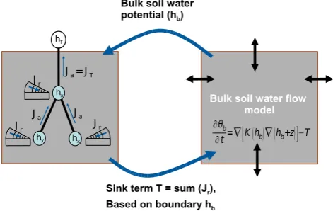
Figure 1 shows the model scheme we use to implement the sink terms into the bulk soil water flow model and how the bulk soil water potential feeds back to the microscale radial soil water flow model. Our concept underlies the assumption that all soil discs around root segments covering a certain soil volumeij k share uniform bulk water potentialψband soil
disc radiirdisc.
The sink termSfor the bulk soil water flow model is cal-culated by summing up the radial fluxesJradm of all soil discs
mbelonging to a certain bulk soil volumeij kas
S(i,j,k)=X
m
Jradm ∀ Jradm ∈ij k
ij k = {(x,y,z)∈R3:ai≤x≤ai+1, bj≤y≤bj+1,ck≤z≤ck+1},
[image:5.595.309.545.61.210.2]withi,j∈ {1...Nhor+1} ⊂Z, k∈ {1...Nvert+1} ⊂Z, where Nhor andNvert are the number of bulk soil volumes in the
Fig. 1. Concept of coupling microscale radial flow to bulk flow
including xylem potentials for a bulk soil volumeij k.
horizontal and vertical direction and the rules forai,bj and
ckare the following
ai=xmin+(i−1)1x; 1x=xmaxN−xmin
hor ;
bj=ymin+(j−1)1y; 1y=ymaxN−ymin
hor ;
ck=zmin+(k−1)1z; 1z=zmaxN−vertzmin.
2.3 The root architecture model
The root architecture model used for our simulations is based on the generic model RootTyp by Pag`es et al. (2004). The generator creates realizations of the same species by simulat-ing growth as a random process coversimulat-ing root emission, axial and radial growth, sequential branching, reiteration, transi-tion, decay and abscission. The interplay of these processes is parameterized plant specifically. We used a parameter set for plant species of sorghum type, which is a class of numer-ous grass species. The size of the root system depends on the stage of plant development, hence age. All generated root systems are characterized by their interconnected root seg-ments of a designated order. The order defines the segseg-ments axial resistance per length (due to alternating xylem vessel elaboration), specific radial resistivity (due to different stages of suberization) and root radius (see Table 1). Figure 2 shows exemplary a root system for one of the 50 realizations. 2.4 The Feddes model
The RWU function of Feddes (like in Feddes et al., 2001) is the following
%(h(x,y,z))=βrw(h)
LaV(x,y,z)
R
V
LaV(x,y,z)dV TPot, (22)
Fig. 2. 2-D-plot of two arbitrarily chosen root system realizations
created by the root architecture generator RootTyp.
rate. To get the volumetric flow rateS(x,y,z), the extrac-tion rate (of volume of water per volume of soil per time)
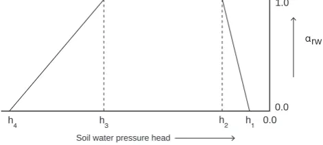
%[m3m−3s−1] has to be applied to a specific soil volume. The Feddes approach includes a water stress functionβrw, where the most common implemented stress function has the form shown in Fig. 3.
2.5 Model input and scenarios
The model exercise was divided into three characteristic cases: (1) the Feddes approach widely applied in current SVAT models based on the RLD neglecting the root sys-tems network character as well as microscopic radial water flow within the soil, the aRoot simulations for (2) Scenario A where higher order roots have higher radial resistances and the aRoot simulations for (3) Scenario B where higher order roots have lower radial resistances (see Table 1). The reason for dividing the aRoot model in two Scenarios (A and B) is the ongoing debate on the range of the radial resistance val-ues (references from Steudle and Peterson, 1998; Zwieniecki et al., 2003).
We performed the simulations for all three cases on 50 root system realizations. The simulation time for root water uptake for all realizations was set to 10 days (with time steps of1t=30 min.) starting from a uniform, initial saturation of2=0.4. The bulk soil water flow model runs on a 2.5×
2.5×2.5 [cm] grid cell size. The overall soil domain size inx-, y- and z-direction is 27.5×27.5×22.5 [cm] among all root realizations. The plants root system age was set to 1 month (28 days) where there was no further root growth applied within the simulation time.
The transpiration rate was assumed to be time invariant withTPot=-8×10⁻¹⁰m3s−1over the 10 days of unlimited uptake, as long as the root collar potential has not exceeded a given threshold. If the corresponding variable collar poten-tial drops below this critical valueψxylemcrit , then the boundary switches from a flux type to a potential type condition and transpirational flux gets variant.
Soil water pressure head
0.0 0.0
1.0
αrw
h₄ h₃ h₂ h₁
Fig. 3. Water stress function used in the Feddes model: Water
up-take aboveh1and below h4 is set to zero due to oxygen deficit and wilting point. Betweenh2and h3 water uptake is maximal (αrw=1). Aboveh2and belowh3, the so-called critical point, wa-ter uptake gets limited where the precise value ofh3is assumed to vary with potential transpiration rateTPot.
The specific radial resistanceζp(as a material constant for
root orderkwith a given thickness of the roots radial path-way) is assumed to decline with increasingkcaused by less suberization, whereζp is calculated by multiplying the ma-terials resistivityχpr with the roots radial thicknessrc. Ra-dial resistanceRris the ratio ofζpto the root outer surface area (Rr=ζp/(2π r0l)[s m−2]). Also, we assume that axial resistance per lengthRlincreases with root order (due to
de-creasing root radius), multiplied by the root segment length
lrit gives the axial resistanceRax=Rl×lr[s m−2].
Parameters of Scenario A are in agreement with measure-ments by Steudle and Peterson (1998)(page 778): Root prop-erties of segment order 2 are referenced by the mature late metaxylem measurements whereas for root order 4 charac-teristics are given by the early metaxylem. For Scenario B ra-dial resistance was decreased, but only for higher order roots, so thatRax/Rris in the range of 0.025 in accordance to the results of Zwieniecki et al. (2003).
3 Results
3.1 Influence of root architecture and hydraulic root parameters on root water uptake behavior
Figure 4 shows the modeled root water uptake (RWU) ver-sus root length density (RLD). The plotted points represent entities on the bulk scale where the RLD was calculated by counting root segment lengths in each bulk soil grid cells and RWU is the given sink term of the bulk soil water flow in Eq. (1). We plotted all model runs (50 realizations of each, the Feddes approach, aRoot Scenario A and aRoot Scenario B) at three different time steps (0, 5 and 10 days).
[image:6.595.310.546.65.171.2]0 0.05 0.1 0.15 0.2 0.25 0.3 0.35 0
0.05 0.1 0.15 0.2 0.25 0.3
Normalized RLD [−]
Normalized sink term [−]
0 0.05 0.1 0.15 0.2 0.25 0.3 0.35 0
0.05 0.1 0.15 0.2 0.25 0.3
Normalized RLD [−]
Normalized sink term [−]
0 0.05 0.1 0.15 0.2 0.25 0.3 0.35 0
0.05 0.1 0.15 0.2 0.25 0.3
Normalized RLD [−]
Normalized sink term [−]
[image:7.595.67.533.63.190.2](a) 0 days (b) 5 days (c) 10 days
Fig. 4. Sink term vs. RLD for 50 Realizations of Scenario A (red square), Scenario B (blue circle) and Feddes (black dot) at (a) initial time
stept=0, (b) after 5 days and (c) after 10 days (sink terms are normalized by the potential transpiration rateTPotand RLD by total root length)
see that Scenarios A and B of aRoot show some compensa-tion effects: water uptake from areas of higher RLD is de-creased and this decline is compensated by inde-creased uptake from lower RLD regions where Scenario B shows a stronger compensation than Scenario A does. Also, att=5 andt=10 days, the sink terms of the Feddes approach and the aRoot Scenarios A and B were comparably similar for higher RLD (between 0.1 and 0.35). Within the range of lower RLD (nor-malized values from 0 to 0.2), water uptake was highest for the Feddes model and lowest for Scenario B. However, in the part of lower RLD (up to 0.1) the sink terms for the Feddes model remained mostly at the 1:1 line with no compensa-tional effects. This missing effects are a straight result of the Feddes model assumptions.
3.2 Influence of root architecture on vertical uptake profiles
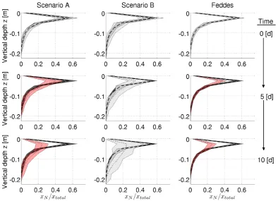
In Fig. 7, we plotted the vertical profiles for RLD and RWU. For this, both variables were averaged over the horizontal soil domain and normalized by the total root length respectively the potential transpiration rateTPot.
All 50 root system realizations showed a similar RLD pro-file resulting in a narrow 90% confidence band. For the aRoot Scenarios A and B, the RWU profiles showed larger con-fidence bands than the RLD profile. Moreover, during the simulation, the confidence intervals for the water uptake pro-files increased in all three cases. The strongest spread could be seen for Scenario B, while the Feddes approach showed only very little variation.
At the initial time step,t=0 days, the mean water uptake profile for both aRoot Scenarios was in the range of the mean RLD profile. The confidence bands showed a slightly higher spread for the uptake profiles than for the RLD profiles. At
t=10 days, the mean uptake at layers with high RLD was for Scenario B only 40% of what would be expected by the RLD profile. At the same time, it was up to 300% higher than RLD at deeper soil layers of lower rooting density. The same
trends were observed for Scenario A but with smaller differ-ences between vertical RWU and RLD because of already limited uptake.
Furthermore, the vertical water uptake profiles of Scenar-ios A and B showed a moving uptake front from layers of high RLD to layers of lower RLD for both scenarios. This shift was faster for Scenario B than for A. Also for Scenario A, RWU was limited earlier than for Scenario B resulting in a slighter compensation of decreased uptake from higher layers (already drier) by increased uptake from lower rooted layers (still wet).
Compared to the aRoot model, we see important differ-ences in the Feddes model: at timestept=0 days the pro-files of vertical uptake do perfectly match the RLD propro-files as can already be seen in Fig. 4a. With time the uptake in the layers of higher RLD decreases but with no compensation of water uptake from less densely rooted layers. The width of the confidence bands remains almost constant in the layers of decreased uptake while they still match the RLD profiles in the nonlimited deeper layers. This general uptake behav-ior leads to early limitation of water uptake compared to the aRoot model.
3.3 Influence of root architecture on critical point of water uptake limitation
Another important factor for modeling root water uptake is the relation between transpirational demand and resulting collar potential (or vice versa). This can only be investigated with a model where xylem potentials are resolved, which is the case for aRoot but not for the Feddes model.
(a) Scenario A (b) Scenario B
Fig. 5. Temporal evolution of collar potentials for (a) Scenario A and (b) Scenario B. The black dotted line is the mean xylem water potential
at the root collar for all 50 realizations. The gray band denotes the 90% confidence interval and the light gray lines are the individual collar potential curves.
also show a high variability among the realizations for Sce-nario A where for B, the confidence interval is narrow for most of the simulation. We also see that plants in Scenario A reach the critical point of limited water uptake much earlier than in Scenario B. There, water uptake is still unlimited at the end of the 10 day long simulations for all realizations.
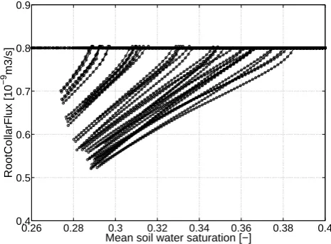
In Fig. 6, we plotted only for Scenario A mean soil sat-uration versus resulting actual transpiration. We observed a wide spread of expected water uptake from individual root architectures. While in early limited root systems uptake was reduced by 40 %, other systems were still not limited after 10 days of transpiration.
4 Discussion
In this model exercise we generated 50 root architectures us-ing the model RootTyp of Pag`es (Pag`es et al., 2004). These realizations could be interpreted as 50 different individuals of the same plant species and age. The obtained root sys-tems show similar root length density profiles, as indicated by the narrow confidence intervals shown in Fig. 7. Root length density decreases exponentially with depth for all in-dividuals. This is in accordance to observations not only for grasses, but for all biomes (Schenk and Jackson, 2002).
For these root systems, root water uptake was simulated over 10 days of transpiration by three model cases: the archi-tecture based aRoot model by Scenarios A and B and the root length based SVAT approach by Feddes. We imple-mented Scenarios A and B both based on current literature in plant physiology (see Steudle and Peterson, 1998; Zwie-niecki et al., 2003). For Scenario A, the specific radial re-sistivity of higher order roots is set within the higher range, where for Scenario B it is at the lower limit. The model re-sults for both Scenarios differ, but both show a confidence spread over all modeled individuals, either regarding the
0.26 0.28 0.3 0.32 0.34 0.36 0.38 0.4 0.4
0.5 0.6 0.7 0.8 0.9
Mean soil water saturation [−]
RootCollarFlux [10
−9
m3/s]
Fig. 6. Individual collar fluxes (black dotted line) for all 50
realiza-tions of Scenario A over mean soil saturation defined as the integral of the entire soil domain (regarding the soil domain as a simple bucket).
evolved collar potential and reaching limiting soil water con-ditions (Scenario A) or regarding the distribution of vertical uptake profiles over soil depth (Scenario B).
[image:8.595.311.544.290.461.2]Fig. 7. Vertical Profiles of RLD (dashed) and RWU (dotted) over soil depth for 50 Realizations of Scenario A (left), B (middle) and Feddes
(right) at time stepst=0 (up), 5 (middle) and 10 (bottom) days. The dark gray band is the 90% confidence interval for the vertical RLD profile, where the light gray band is the 90% confidence interval for the RWU profile (transparent red bands denote limited water uptake).
(concerning the temporal evolution of collar potentials, Sce-nario A) or on the soils side (concerning the vertical uptake profiles, Scenario B).
In our aRoot simulations the modeled root water uptake moves from densely to less densely rooted layers with time. This is in agreement with observation (Garrigues et al., 2006; Lai and Katul, 2000) as well as with results from detailed 3-D models for root water uptake (3-Doussan et al., 2006; Javaux et al., 2008). Our results suggest that the dynamic of this shift depends on the individual root architecture as well as on root properties (here the range of radial resistances). The Feddes approach does not show this moving uptake behavior (as the model does not consider such effects) and additionally lacks the architecture based scattering in water uptake rates versus RLD. Javaux et al. (2008) already pointed out, the parameterization of the Feddes model seems to have little biophysical basis. Our results support this interpretation.
Our simulations show that the occurrence of decreasing water uptake is not at a unique critical point in soil water potential (corresponding to pointψ3in Fig. 3). This was the case, although we used the same soil environment and same plant species (with similar RLD profiles). Rather, this study shows that root architecture influences the critical point of bulk soil water content where water uptake becomes limiting. The diverse access of the root systems hydraulic active roots to the soil water storage explains this model result.
The proposed model aRoot underlies certain assumptions or simplifications. Schr¨oder et al. (2008) has shown, that the local soil hydraulic conductivity drop around the roots be-comes important when increasing the size of the bulk soil grid cells. We accounted for this by implementing a mi-croscale radial flow model coupled to the bulk soil water flow. In their model study, Schr¨oder et al. (2009) concluded that for coarser soil discretization, separating the microscale (radial) flow from bulk soil water flow as done in aRoot (sim-ilar to their method C) gave the best results compared to fine discretized RWU models. The assumption of uniform bulk water content and soil disc radii for all soil discs covering a certain soil volume is discussed in de Jong van Lier et al. (2006). Further work would be necessary to quantify the in-fluence of this assumption.
Table 2. List of Variables and Abbreviations.
Symbol Units Description
r m radial distance
x,y,z m cartesian coordinates
lr m root segment length
t s time
ψ m matric potential
8 m2s−1 matric flux potential
θ m3m−3 volumetric water content
J,T ,S m3s−1 volumetric flow rates
K m s−1 hydraulic conductivity
R s m−2 hydraulic resistance κ m2s−1 hydraulic conductance
LaV [m m−3] accumulated root length per volume (RLD) RLD root length density
RWU root water uptake
5 Conclusions
In this chapter we developed a simplified model, that cap-tures small scale feacap-tures of plant-water uptake but is still computationally fast. Although our model currently runs with a 3-D Richards Model it is intended for later imple-mentation in SVAT schemes and for testing hypotheses on optimal root behavior in different environments.
With our model, we found a wide range of vertical wa-ter uptake profiles even for very similar vertical RLD pro-files, which is a result of the individual behavior of each root architecture and its hydraulic parameters. Root architecture becomes more important for the spatial distribution of uptake with time as shown by the increase of confidence bands for the vertical uptake profiles.
The model predictions with the architecture based model aRoot show different behavior than the Feddes Model. The Feddes model distributes and limits root water uptake based on two key properties of the plant or plant community: (1) the root length density profile, and (2) the critical point where water uptake starts to be limited by soil moisture (seeψ3in Fig. 3). Our modeling results with aRoot suggest that both of these properties are not suitable for describing the distribu-tion of real water uptake. While the root length density dis-tribution was similar for all 50 root system realizations, root water uptake profiles differed considerably between individ-uals. This was especially the case, when assuming relatively low values of root radial resistance (scenario B). Also, tran-spiration started to be limited at a wide range of bulk water contents, particularly for scenario A, where large root radial resistance was assumed.
Our results suggest that root water uptake behavior might vary greatly between individuals of a particular species. More research is necessary to support this conclusion, and to identify such root properties, which are suitable for describing root water uptake profiles. Also, roots have a
complex effect on soil water content and the flow of water through the soil by roots, especially if the interaction be-tween root growth and the surrounding soil is considered. In case of roots clustering in a certain soil volume this might significantly affect the pore space distribution, further im-pacting on the water holding and soil water movement char-acteristics.
Acknowledgements. We thank Doris Vetterlein, Andrea Carmi-nati, Mathieu Javaux, Tom Schr¨oder, Vanessa Dunbabin and Jan W. Hopmans for early discussion and comments. This work was kindly supported by Helmholtz Impulse and Networking Fund through Helmholtz Interdisciplinary Graduate School for Environmental Research (HIGRADE).
Edited by: N. Romano and C. Hinz
References
Amenu, G. G. and Kumar, P.: A model for hydraulic redistribution incorporating coupled soil-root moisture transport, Hydrol. Earth Syst. Sci., 12, 55–74, 2008,
http://www.hydrol-earth-syst-sci.net/12/55/2008/.
Clausnitzer, V. and Hopmans, J. W.: Simultaneous modeling of transient three-dimensional root growth and soil water flow, Plant Soil, 164, 299–314, 1994.
de Jong van Lier, Q., Metselaar, K., and van Dam, J. C.: Root wa-ter extraction and limiting soil hydraulic conditions estimated by numerical simulation, Vadose Zone J., 5, 1264–1277, doi: 10.2136/vzj2006.0056, 2006.
de Jong van Lier, Q., van Dam, J. C., Metselaar, K., de Jong, R., and Duijnisveld, W. H. M.: Macroscopic Root Water Uptake Distri-bution Using a Matric Flux Potential Approach, Vadose Zone J., 7, 1065–1078, 2008.
De Willigen, P. and van Noordwijk, M.: Root, Plant. Production and Nutrient Use Efficiency, Ph.D. thesis, Agricultural Univer-sity, Wageningen, The Netherlands, 1987.
Desborough, C. E.: The impact of root weighting on the re-sponse of transpiration to moisture stress in land surface schemes, Mon. Weather Rev., 125(8), 1920–1930, doi:10.1175/ 1520-0493(1997)125h1920:TIORWOi2.0.CO;2, 1997.
Doussan, C., Pag`es, L., and Vercambre, G.: Modelling of the Hy-draulic Architecture of Root Systems: an Integrated Approach to Water Absorption – Model Description, Ann. Bot.-London, 81, 213–223, 1998.
Doussan, C., Pierret, A., Garrigues, E., and Pag`es, L.: Water up-take by plant roots: II – Modelling of water transfer in the soil root-system with explicit account of flow within the root system – Comparison with experiments, Plant Soil, 283(1–2), 99–117, doi:10.1007/s11104-004-7904-z, 2006.
Feddes, R., Kowalik, P., Kolinska-Malinka, K., and Zaradny, H.: Simulation of field water uptake by plants using a soil water de-pendent root extraction function, J. Hydrol., 31, 13–26, 1976. Feddes, R. A., Hoff, H., Bruen, M., Dawson, T., de Rosnay, P.,
Gardner, W. R.: Dynamics aspects of water availability to plants, Soil Sci., 89, 63–73, 1960.
Gardner, W. R.: Relation of root distribution to water uptake and availabilty, Agron. J., 56, 41–45, 1964.
Garrigues, E., Doussan, C., and Pierret, A.: Water Uptake by Plant Roots: I - Formation and Propagation of a Water Ex-traction Front in Mature Root Systems as Evidenced by 2-D Light Transmission Imaging, Plant Soil, 283(1–2), 83–98, doi: 10.1007/s11104-004-7903-0, 2006.
Green, S. R. and Clothier, B.: Root water uptake by kiwifruit vines following partial wetting of the root zone, Plant Soil, 173, 317– 328, doi:10.1007/BF00011470, 1995.
Jacobsen, B.: Water and phosphate transport to plant roots, Acta Agr. Scand., 24, 55–60, 1974.
Javaux, M., Schr¨oder, T., Vanderborght, J., and Vereecken, H.: Use of a Three-Dimensional Detailed Modeling Approach for Pre-dicting Root Water Uptake, Vadose Zone J., 7, 1079–1089, doi: 10.2136/vzj2007.0115, 2008.
Kolditz, O., Delfs, J.-O., B¨urger, C., Beinhorn, M., and Park, C.-H.: Numerical analysis of coupled hydrosystems based on an object-oriented compartment approach, J. Hydroinform., 10(3), 227–244, doi:DOI:10.2166/hydro.2008.003, 2008.
Lai, C.-T. and Katul, G.: The dynamic role of root-water up-take in coupling potential to actual transpiration, Adv. Wa-ter Resour., 23(4), 427–439, doi:doi:10.1016/S0309-1708(99) 00023-8, 2000.
Levin, A., Shaviv, A., and Indelman, P.: Influence of root re-sistivity on plant water uptake mechanism, part I: numeri-cal solution, Transport Porous Med., 70, 63–79, doi:10.1007/ s11242-006-9084-1, 2007.
Li, K., Jong, R. D., and Boisvert, J.: An exponential root-water-uptake model with water stress compensation, J. Hydrol., 252, 189–204, 2001.
Pag`es, L., Vercambre, G., Drouet, J.-L., Lecompte, F., Collet, C., and Bot, J. L.: Root Typ: a generic model to depict and analyse the root system architecture, Plant Soil, 258, 103–119, 2004. Schenk, H. and Jackson, R.: The global biogeography of roots,
Ecol. Monogr., 72(3), 311–328, 2002.
Schr¨oder, T., Javaux, M., Vanderborght, J., K¨orfgen, B., and H. Vereecken, H.: Effect of local soil hydraulic conductivity drop using a 3-D root water uptake model, Vadose Zone J., 7, 1089– 1098, doi:10.2136/vzj2007.0114, 2008.
Schr¨oder, T., Javaux, M., Vanderborght, J., K¨orfgen, B., and H. Vereecken, H.: Implementation of a microscopic soil-root hy-draulic conductivity drop function in a 3-D soil-root architecture water transfer model, Vadose Zone J., 8, 783–792, 2009. Schymanski, S. J., Sivapalan, M., Roderick, M. L., Beringer, J., and
Hutley, L. B.: An optimality-based model of the coupled soil moisture and root dynamics, Hydrol. Earth Syst. Sci., 12, 913– 932, 2008,
http://www.hydrol-earth-syst-sci.net/12/913/2008/.
Sharp, R. E. and Davies, W. J.: Root Growth and Water Uptake by Maize Plants in Drying Soil, http://jxb.oxfordjournals.org/cgi/ content/abstract/36/9/1441, J. Exp. Bot., 36(170), 1441–1456, 1985.
Siqueira, M., Katul, G., and Porporato, A.: Onset of water stress, hysteresis in plant conductance, and hydraulic lift: Scaling soil water dynamics from millimeters to meters, Water Resour. Res., 44, W01432, doi:10.1029/2007WR006094, 2008.
ˇSim˚unek, J., van Genuchten, M. Th., and ˇSejna, M.: The HYDRUS Software Package for Simulating Two- and Three-dimensional Movement of Water, Heat, and Multiple Solutes in Variably-saturated Media, Technical Manual, Version 1.0, PC Progress, Prague, Czech Republic, p. 241, 2006.
ˇSim˚unek, J., ˇSejna, M., Saito, H., Sakai, M., and van Genuchten, M. Th.: The HYDRUS-1D Software Package for Simulating the Movement of Water, Heat, and Multiple Solutes in Variably Sat-urated Media, Version 4.0, HYDRUS Software Series 3, Depart-ment of EnvironDepart-mental Sciences, University of California River-side, RiverRiver-side, California, USA, p. 315, 2008.
ˇSim˚unek, J. and Hopmans, J. W.: Modeling compensated root water and nutrient uptake, Ecol. Model., 220, 505–520, doi:10.1016/j. ecolmodel.2008.11.004, 2009.
Sperry, J. S., Stiller, V., and Hacke, U. G.: Xylem hydraulics and the Soil-Plant-Atmosphere Continuum: Opportunities and Un-resolved Issues, http://agron.scijournals.org/cgi/content/abstract/ 95/6/1362, Agron. J., , 95(6), 1362–1370, 2003.
Steudle, E.: Water uptake by plant roots: An integration of views, Plant Soil, 226, 45–56, 2000.
Steudle, E. and Peterson, C. A.: How does water get through roots?, http://jxb.oxfordjournals.org/cgi/content/abstract/49/322/775, J. Exp. Bot., 49(322), 775–788, 1998.
Teuling, A. J., Uijlenhoet, R., Hupet, F., and Troch, P. A.: Impact of plant water uptake strategy on soil moisture and evapotranspira-tion dynamics during drydown, Geophys. Res. Lett., 33, L03401, doi:10.1029/2005GL025019, 2006.
Tuzet, A., Perrier, A., and Leuning, R.: A coupled model of stom-atal conductance, photosynthesis and transpiration, Plant Cell Environ., 26, 1097–1116, doi:10.1046/j.1365-3040.2003.01035. x, 2003.
van Genuchten, M.: A closed-form equation for predicting the hy-draulic conductivity of unsaturated soils, Soil Sci. Soc. Am. J., 44, 892–898, 1980.
Vrugt, J. A., van Wijk, M. T., Hopmans, J. W., and ˇSimunek, J.: One-, two-, and three-dimensional root water uptake func-tions for transient modeling, http://www.agu.org/journals/wr/ v037/i010/2000WR000027/, Water Resour. Res., 37 (10), 2457– 2470, 2001.
Wan, C., Yilmaz, I., and Sosebee, R.: Seasonal soil-water availabil-ity influences snakeweed root dynamics, J. Arid Environ., 51, 255–264, doi:10.1016/jare.2001.0942, 2002.
Zeng, X., Dai, Y., Dickinson, R., and Shaikh, M.: The role of root distribution for climate simulation over land, http: //www.agu.org/pubs/crossref/1998/1998GL900216.shtml, Geo-phys. Res. Lett., 25(24), 4533–4536, 1998.