Efficient output solution for nonlinear stochastic optimal control problem with model reality differences

(1)

Research Article

Efficient Output Solution for Nonlinear Stochastic Optimal

Control Problem with Model-Reality Differences

Sie Long Kek,

1

Kok Lay Teo,

2

and Mohd Ismail Abdul Aziz

3

1_{Department of Mathematics and Statistics, Universiti Tun Hussein Onn Malaysia, 86400 Parit Raja, Malaysia} 2_{Department of Mathematics and Statistics, Curtin University of Technology, Perth, WA 6845, Australia} 3_{Department of Mathematical Sciences, Universiti Teknologi Malaysia (UTM), 81310 Skudai, Malaysia} Correspondence should be addressed to Sie Long Kek; slkek@uthm.edu.my

Received 8 August 2014; Revised 15 October 2014; Accepted 16 October 2014

Academic Editor: Hamid R. Karimi

Copyright © Sie Long Kek et al. This is an open access article distributed under the Creative Commons Attribution License, which permits unrestricted use, distribution, and reproduction in any medium, provided the original work is properly cited.

A computational approach is proposed for solving the discrete time nonlinear stochastic optimal control problem. Our aim is to obtain the optimal output solution of the original optimal control problem through solving the simplified model-based optimal control problem iteratively. In our approach, the adjusted parameters are introduced into the model used such that the differences between the real system and the model used can be computed. Particularly, system optimization and parameter estimation are integrated interactively. On the other hand, the output is measured from the real plant and is fed back into the parameter estimation problem to establish a matching scheme. During the calculation procedure, the iterative solution is updated in order to approximate the true optimal solution of the original optimal control problem despite model-reality differences. For illustration, a wastewater treatment problem is studied and the results show the efficiency of the approach proposed.

1. Introduction

Many real world problems can be formulated as the stochastic dynamical systems [1–3]. In presence of the random noises, the exact state trajectory is impossible to be obtained. The output sequence, which is measured from the process plant, is also disturbed unavoidably. Since the fluctuation behavior of the output sequence would be the actual outcome, obtaining such outcome from a mathematical model is a challenging task. In stochastic system, estimation, identification, and adaptive control are the general techniques [4]. Particularly, the Kalman filtering theory and the extended Kalman filter give a great impact in studying stochastic systems, both for linear and nonlinear cases [5–8]. The data-driven method that could be applied in the fault diagnosis provides an efficient identification approach for stochastic systems. Using the process data to identify the parameters without knowing the actual process model is one of the advantages in modeling stochastic systems [9]. In addition, the stochastic switching systems, subject to random abrupt changes in their dynamics,

attract the researchers to design, model, control, and optimize

the stochastic systems [10,11].

The use of stochastic systems, therefore, plays the impor-tant role in the real world applications. The development of solution methods and the corresponding practical analysis are contributed to the stochastic research communities, ranging from engineering to business. From the literature, the applications of stochastic system have been well defined; see, for example, power management [12], portfolio selec-tion [13], financial market debt crises [14], insurance with bankruptcy return [15], annuity contracts [16], natural gas networks [17], brain-machine interface operation [18], multi-degree-of-freedom systems [19], fleet composition problem [20], fault diagnosis [21], network control system [22], and stochastic switching system [23–25].

In this paper, we propose a computational approach for optimal control of the nonlinear stochastic dynamical system in discrete time. Our aim is to obtain the optimal output solution of the original optimal control problem from a mathematical model. In doing so, a model-based optimal

(2)

control problem is simplified from the original optimal control problem. Furthermore, the adjusted parameters are introduced into the model used. In this way, the differences between the real system and the model used can be computed. Thus, system optimization and parameter estimation are integrated interactively. On the other hand, the output, which is measured from the real plant, is fed back into the param-eter estimation problem. This operation is implemented to establish a matching scheme, in turn, updating the optimal solution of the model used at each iteration step. Notice that the application of this operation, which is the advantage of the algorithm proposed, is in contrast to the works discussed in [26–28], where the real output is fed back into the system optimization problem. When convergence is achieved, the iterative solution approximates to the true optimal solution of the original optimal control problem, in spite of model-reality differences. Hence, the efficiency of the approach proposed is highly recommended.

The rest of the paper is organized as follows. InSection 2,

a discrete time nonlinear stochastic optimal control problem is described and the corresponding model-based optimal

control problem is simplified. In Section 3, an expanded

optimal control model, which integrates system optimization and parameter estimation interactively, is introduced. Then, the iterative algorithm based on principle of model-reality differences is derived, and the computation procedure is

sum-marized. InSection 4, a convergence analysis is provided. In

Section 5, an example of the optimal control of a wastewater treatment problem is illustrated. Finally, some concluding remarks are made.

2. Problem Statement

Consider the following discrete time nonlinear stochastic optimal control problem:

min

𝑢(𝑘) 𝐽0(𝑢)

= 𝐸 [𝜑 (𝑥 (𝑁) , 𝑁) +𝑘−1∑

𝑘=0𝐿 (𝑥 (𝑘) , 𝑢 (𝑘) , 𝑘)]

subject to 𝑥 (𝑘 + 1) = 𝑓 (𝑥 (𝑘) , 𝑢 (𝑘) , 𝑘) + 𝐺𝜔 (𝑘) ,

𝑦 (𝑘) = ℎ (𝑥 (𝑘) , 𝑘) + 𝜂 (𝑘) ,

(1)

where𝑢(𝑘) ∈R𝑚,𝑘 = 0, 1, . . . , 𝑁 − 1,𝑥(𝑘) ∈ R𝑛,𝑘 = 0, 1,

. . . , 𝑁, and 𝑦(𝑘) ∈ R𝑝, 𝑘 = 0, 1, . . . , 𝑁, are, respectively, the control sequence, the state sequence, and the output

sequence.𝜔(𝑘) ∈R𝑞,𝑘 = 0, 1, . . . , 𝑁 − 1, and𝜂(𝑘) ∈R𝑝,𝑘 =

0, 1, . . . , 𝑁, are the stationary Gaussian white noise sequences

with zero mean and their covariances are given by𝑄_𝜔∈R𝑞×𝑞

and𝑅_𝜂 ∈ R𝑝×𝑝, which are positive definite matrices.𝐺 ∈

R𝑛×𝑞_{is a process coefficient matrix,}_{𝑓 :}_R𝑛_×_R𝑚_×_R _→ _R𝑛

represents the real plant, andℎ : R𝑛 ×R → R𝑝 is the

output measurement.𝐽₀is the scalar cost function and𝐸[⋅]

is the expectation operator, whereas𝜑 : R𝑛 ×R → R

is the terminal cost and 𝐿 : R𝑛 ×R𝑚 ×R → R is the

cost under summation. It is assumed that all functions in(1)

are continuously differentiable with respect to their respective arguments.

The initial state is

𝑥 (0) = 𝑥0, (2)

where𝑥₀∈R𝑛is a random vector with mean and covariance

given, respectively, by

𝐸 [𝑥₀] = 𝑥₀,

𝐸 [(𝑥₀− 𝑥₀) (𝑥₀− 𝑥₀)T

] = 𝑀₀. (3)

Here,𝑀₀ ∈ R𝑛×𝑛is a positive definite matrix. It is assumed

that initial state, process noise, and measurement noise are statistically independent.

This problem is referred to as Problem(𝑃).

Because of the complexity in the structure of the real plant and the presence of the random sequences, the exact solution

of Problem (𝑃) is impossible to be obtained. Moreover,

applying the nonlinear filtering theory to estimate the state dynamics is computationally demanding. In view of these, we propose a simplified model-based optimal control problem, which is constructed by carrying out the linearization of

Problem (𝑃), in order to approximate the correct optimal

solution of the original optimal control problem iteratively. This simplified model-based optimal control problem, which

is referred to as Problem(𝑀), is given by

min

𝑢(𝑘) 𝐽1(𝑢) =

1 2𝑥 (𝑁)

T_{𝑆 (𝑁) 𝑥 (𝑁) + 𝛾 (𝑁)}

+𝑁−1∑

𝑘=0

1 2(𝑥 (𝑘)

T_{𝑄𝑥 (𝑘) + 𝑢 (𝑘)}T_{𝑅𝑢 (𝑘))}

+ 𝛾 (𝑘)

subject to 𝑥 (𝑘 + 1) = 𝐴𝑥 (𝑘) + 𝐵𝑢 (𝑘) + 𝛼₁(𝑘) ,

𝑦 (𝑘) = 𝐶𝑥 (𝑘) + 𝛼2(𝑘) ,

𝑥 (0) = 𝑥0,

(4)

where𝑥(𝑘) ∈ R𝑛, 𝑘 = 0, 1, . . . , 𝑁, and𝑦(𝑘) ∈ R𝑝, 𝑘 =

0, 1, . . . , 𝑁, are the expected state sequence and the expected

output sequence, respectively.𝛼₁(𝑘) ∈R𝑛, 𝑘 = 0, 1, . . . , 𝑁 −

1, 𝛼₂(𝑘) ∈ R𝑝, 𝑘 = 0, 1, . . . , 𝑁, and 𝛾(𝑘) ∈ R, 𝑘 =

0, 1, . . . , 𝑁, are adjustable parameters. 𝐴 ∈ R𝑛×𝑛 is a state

transition matrix,𝐵 ∈ R𝑛×𝑚 is a control coefficient matrix,

and𝐶 ∈ R𝑝×𝑛is an output coefficient matrix, while𝑆(𝑁) ∈

R𝑛×𝑛_and_{𝑄 ∈} _R𝑛×𝑛 _{are positive semidefinite matrices and}

𝑅 ∈R𝑚×𝑚_{is a positive definite matrix.}

Notice that, without the adjustable parameters, Problem

(𝑀)is a standard linear quadratic regulator (LQR) optimal

(3)

3. System Optimization with

Parameter Estimation

Now, let us introduce an expanded optimal control problem,

which is referred to as Problem(𝐸), given as follows:

min

𝑢(𝑘) 𝐽2(𝑢) =

1 2𝑥 (𝑁)

T

𝑆 (𝑁) 𝑥 (𝑁) + 𝛾 (𝑁)

+𝑁−1∑

𝑘=0

1 2(𝑥 (𝑘)

T_{𝑄𝑥 (𝑘) + 𝑢 (𝑘)}T_{𝑅𝑢 (𝑘))}

+ 𝛾 (𝑘) +1₂𝑟₁‖𝑢 (𝑘) −V(𝑘)‖2

+1

2𝑟2‖𝑥 (𝑘) − 𝑧 (𝑘)‖2

𝑦 (𝑘) = 𝐶𝑥 (𝑘) + 𝛼2(𝑘) ,

𝑥 (0) = 𝑥0,

1 2𝑧 (𝑁)

T

𝑆 (𝑁) 𝑧 (𝑁) + 𝛾 (𝑁) = 𝜑 (𝑧 (𝑁) , 𝑁) ,

1 2(𝑧 (𝑘)

T_{𝑄𝑧 (𝑘) +}_V_(𝑘)T_𝑅_V_{(𝑘)) + 𝛾 (𝑘)}

= 𝐿 (𝑧 (𝑘) ,V(𝑘) , 𝑘) ,

𝐴𝑧 (𝑘) + 𝐵V(𝑘) + 𝛼₁(𝑘) = 𝑓 (𝑧 (𝑘) ,V(𝑘) , 𝑘) , 𝐶𝑧 (𝑘) + 𝛼2(𝑘) = 𝑦 (𝑘) ,

V(𝑘) = 𝑢 (𝑘) , 𝑧 (𝑘) = 𝑥 (𝑘) ,

(5)

whereV(𝑘) ∈ R𝑚, 𝑘 = 0, 1, . . . , 𝑁 − 1, and𝑧(𝑘) ∈R𝑛, 𝑘 =

0, 1, . . . , 𝑁, are introduced to separate the control and the expected state from the respective signals in the parameter

estimation problem and‖ ⋅ ‖ denotes the usual Euclidean

norm. The terms(1/2)𝑟₁‖𝑢(𝑘) −V(𝑘)‖2 and(1/2)𝑟₂‖𝑥(𝑘) −

𝑧(𝑘)‖2are introduced to improve convexity and enhance con-vergence of the resulting iterative algorithm. It is important to note that the algorithm is to be designed such that the

constraintsV(𝑘) = 𝑢(𝑘)and𝑧(𝑘) = 𝑥(𝑘)will be satisfied at

the end of the iterations. In this situation, the state estimate

𝑧(𝑘)and the controlV(𝑘)will be used for the computation

in the parameter estimation and the matching schemes. On

the other hand, the corresponding expected state𝑥(𝑘) and

control𝑢(𝑘)will be reserved for optimizing the model-based

optimal control problem.

It is important to note that the output measured from the real plant is fed back into the parameter estimation problem and the matching scheme, which aims at updating the model output from the model-based optimal control problem repeatedly. On this basis, the output residual could be reduced such that the model output approximates closely to the real output, in spite of model-reality differences. This

improvement enhances the accuracy of the output solution as discussed in [26–28].

3.1. Optimality Conditions. Define the Hamiltonian function

for Problem(𝐸)as follows [28–30]:

𝐻 (𝑘) = 1₂(𝑥 (𝑘)T_{𝑄𝑥 (𝑘) + 𝑢 (𝑘)}T_{𝑅𝑢 (𝑘)) + 𝛾 (𝑘)}

+1₂𝑟1‖𝑢 (𝑘) −V(𝑘)‖2+1₂𝑟2‖𝑥 (𝑘) − 𝑧 (𝑘)‖2

− 𝜆 (𝑘)T

𝑢 (𝑘) − 𝛽 (𝑘)T 𝑥 (𝑘) + 𝑞 (𝑘)T_{(𝐶𝑥 (𝑘) + 𝛼}

2(𝑘) − 𝑦 (𝑘))

+ 𝑝 (𝑘 + 1)T_{(𝐴𝑥 (𝑘) + 𝐵𝑢 (𝑘) + 𝛼}

1(𝑘)) .

(6)

Then, the augmented cost function becomes

𝐽₂󸀠(𝑘) = 1₂𝑥 (𝑁)T

𝑆 (𝑁) 𝑥 (𝑁) + 𝛾 (𝑁)

+ 𝑝 (0)T

𝑥 (0) − 𝑝 (𝑁)T

𝑥 (𝑁) + 𝜉 (𝑁)

× (𝜑 (𝑧 (𝑁) , 𝑁) −1₂𝑧 (𝑁)T

𝑆 (𝑁) 𝑧 (𝑁) − 𝛾 (𝑁))

+ ΓT_{(𝑥 (𝑁) − 𝑧 (𝑁))}

+𝑁−1∑

𝑘=0

𝐻 (𝑘) − 𝑝 (𝑘)T_{𝑥 (𝑘)+ 𝜆 (𝑘)}T_V_{(𝑘)+ 𝛽 (𝑘)}T_{𝑧 (𝑘)}

+ 𝜉 (𝑘) (𝐿 (𝑧 (𝑘) ,V(𝑘) , 𝑘)

−1₂(𝑧 (𝑘)T

𝑄𝑧 (𝑘) +V(𝑘)T_𝑅_V_(𝑘))

−𝛾 (𝑘))

+ 𝜇 (𝑘)T_{(𝑓 (𝑧 (𝑘) ,}_V_{(𝑘) , 𝑘) − 𝐴𝑧 (𝑘)} −𝐵V(𝑘) − 𝛼₁(𝑘))

+ 𝜋 (𝑘)T

(𝑦 (𝑘) − 𝐶𝑧 (𝑘) − 𝛼2(𝑘)) ,

(7)

where 𝑝(𝑘), 𝑞(𝑘), 𝜉(𝑘), 𝜇(𝑘), 𝜋(𝑘), Γ, 𝜆(𝑘), and 𝛽(𝑘) are the

appropriate multipliers to be determined later.

Applying the calculus of variation [26,27,29–31] to(7),

the following necessary optimality conditions are obtained.

(a) Stationary condition:

𝑅𝑢 (𝑘) + 𝐵T_{𝑝 (𝑘 + 1) − 𝜆 (𝑘) − 𝑟}

1(V(𝑘) − 𝑢 (𝑘)) = 0. (8a)

(b) Costate equation:

𝑝 (𝑘) = 𝑄𝑥 (𝑘) + 𝐴T

𝑝 (𝑘 + 1) − 𝛽 (𝑘) − 𝑟2(𝑧 (𝑘) − 𝑥 (𝑘)) .

(4)

(c) State equation:

𝑥 (𝑘 + 1) = 𝐴𝑥 (𝑘) + 𝐵𝑢 (𝑘) + 𝛼1(𝑘) (8c)

with the boundary conditions𝑥(0) = 𝑥₀and𝑝(𝑁) =

Γ.

(d) Adjustable parameter equations:

𝜑 (𝑧 (𝑁) , 𝑁) = 1₂𝑧 (𝑁)T

𝑆 (𝑁) 𝑧 (𝑁) + 𝛾 (𝑁) , (9a)

𝐿 (𝑧 (𝑘) ,V(𝑘) , 𝑘)

=1₂(𝑧 (𝑘)T

𝑄𝑧 (𝑘) +V(𝑘)T_𝑅_V_{(𝑘)) + 𝛾 (𝑘) ,}

(9b)

𝑓 (𝑧 (𝑘) ,V(𝑘) , 𝑘) = 𝐴𝑧 (𝑘) + 𝐵V(𝑘) + 𝛼₁(𝑘) , (9c)

𝑦 (𝑘) = 𝐶𝑧 (𝑘) + 𝛼2(𝑘) . (9d)

(e) Multiplier equations:

Γ = ∇_𝑧(𝑘)𝜑 − 𝑆 (𝑁) 𝑧 (𝑁) , (10a)

𝜆 (𝑘) = − (∇V(𝑘)𝐿 − 𝑅V(𝑘)) − (_𝜕_V𝜕𝑓_(𝑘)− 𝐵)

T

̂𝑝 (𝑘 + 1) ,

(10b)

𝛽 (𝑘) = − (∇𝑧(𝑘)𝐿 − 𝑄𝑧 (𝑘)) − (_{𝜕𝑧 (𝑘)}𝜕𝑓 − 𝐴)

T

̂𝑝 (𝑘 + 1)

(10c)

with𝜉(𝑘) = 1, 𝜇(𝑘) = ̂𝑝(𝑘 + 1), and𝜋(𝑘) = 𝑞(𝑘) = 0.

(f) Separable variables:

V(𝑘) = 𝑢 (𝑘) , 𝑧 (𝑘) = 𝑥 (𝑘) , ̂𝑝 (𝑘) = 𝑝 (𝑘) . (11)

In view of these necessary optimality conditions,

condi-tions(8a),(8b), and(8c)are the necessary conditions for the

modified model-based optimal control problem, conditions

(9a), (9b), (9c), and (9d) define the parameter estimation

problem, and conditions(10a),(10b), and(10c)are used to

compute the multipliers.

3.2. Feedback Control Law. Taking the necessary optimality

conditions (8a), (8b), and (8c), the modified model-based

optimal control problem, which is referred to as Problem

(𝑀𝑀), is defined as follows:

min

𝑢(𝑘) 𝐽3(𝑢) =

1 2𝑥 (𝑁)

T_{𝑆 (𝑁) 𝑥 (𝑁) + 𝛾 (𝑁) + Γ}T_{𝑥 (𝑁)}

+𝑁−1∑

𝑘=0

1 2(𝑥 (𝑘)

T_{𝑄𝑥 (𝑘) + 𝑢 (𝑘)}T_{𝑅𝑢 (𝑘))}

+ 𝛾 (𝑘) +1₂𝑟₁‖𝑢 (𝑘) −V(𝑘)‖2

+1

2𝑟2‖𝑥 (𝑘) − 𝑧 (𝑘)‖2 − 𝜆 (𝑘)T_{𝑢 (𝑘) − 𝛽 (𝑘)}T_{𝑥 (𝑘)}

𝑦 (𝑘) = 𝐶𝑥 (𝑘) + 𝛼2(𝑘) ,

𝑥 (0) = 𝑥0.

(12)

To solve Problem (𝑀𝑀), we will construct a feedback

control law, which includes the model-reality differences for system optimization. Hence, with the determined value of the adjustable parameters, the corresponding result is stated in the following theorem.

Theorem 1 (expanded optimal control law). Suppose that the

expanded optimal control law for Problem(𝐸)exists. Then, this

optimal control law is the feedback control law for Problem

(𝑀𝑀)given by

𝑢 (𝑘) = −𝐾 (𝑘) 𝑥 (𝑘) + 𝑢𝑓𝑓(𝑘) , (13)

where

𝑢_𝑓𝑓(𝑘) = − (𝑅_𝑎+ 𝐵T

𝑆 (𝑘 + 1) 𝐵)−1

× (𝐵T_{𝑠 (𝑘 + 1) + 𝐵}T_{𝑆 (𝑘 + 1) 𝛼}

1(𝑘) − 𝜆𝑎(𝑘)) ,

(14a)

𝐾 (𝑘) = (𝑅𝑎+ 𝐵T𝑆 (𝑘 + 1) 𝐵)−1𝐵T𝑆 (𝑘 + 1) 𝐴, (14b)

𝑆 (𝑘) = 𝑄𝑎+ 𝐴T𝑆 (𝑘 + 1) (𝐴 − 𝐵𝐾 (𝑘)) , (14c)

𝑠 (𝑘) = (𝐴 − 𝐵𝐾 (𝑘))T

(𝑠 (𝑘 + 1) + 𝑆 (𝑘 + 1) 𝛼1(𝑘))

+ 𝐾 (𝑘)T_𝜆

𝑎(𝑘) − 𝛽𝑎(𝑘)

(14d)

with the boundary conditions𝑆(𝑁)given and𝑠(𝑁) = 0, and

𝑅_𝑎= 𝑅 + 𝑟₁𝐼_𝑚; 𝑄_𝑎= 𝑄 + 𝑟₂𝐼_𝑛;

𝜆_𝑎(𝑘) = 𝜆 (𝑘) + 𝑟1V(𝑘) ; 𝛽𝑎(𝑘) = 𝛽 (𝑘) + 𝑟2𝑧 (𝑘) .

(15)

Proof. From(8a), the stationary condition can be rearranged

by

𝑅_𝑎𝑢 (𝑘) = −𝐵T_{𝑝 (𝑘 + 1) + 𝜆}

(5)

Applying the sweep method [28,30,31], that is,

𝑝 (𝑘) = 𝑆 (𝑘) 𝑥 (𝑘) + 𝑠 (𝑘) , (17)

substitute(17)for𝑘 = 𝑘 + 1into(16)to yield

𝑅𝑎𝑢 (𝑘) = −𝐵T𝑆 (𝑘 + 1) 𝑥 (𝑘 + 1) − 𝐵T𝑠 (𝑘 + 1) + 𝜆𝑎(𝑘) .

(18)

Then, consider the state equation (8c)in (18). After some

algebraic manipulations, the feedback control law (13) is

obtained, where(14a)and(14b)are satisfied.

From (8b), the costate equation is rewritten as follows

after substituting(17)for𝑘 = 𝑘 + 1into(8b):

𝑝 (𝑘) = 𝑄𝑎𝑥 (𝑘) + 𝐴T𝑆 (𝑘 + 1) 𝑥 (𝑘 + 1)

+ 𝐴T_{𝑠 (𝑘 + 1) − 𝛽}

𝑎(𝑘) .

(19)

Considering the state equation(8c)in(19), we have

𝑝 (𝑘) = 𝑄𝑎𝑥 (𝑘) + 𝐴T𝑆 (𝑘 + 1) (𝐴𝑥 (𝑘) + 𝐵𝑢 (𝑘) + 𝛼1(𝑘))

+ 𝐴T_{𝑠 (𝑘 + 1) − 𝛽}

𝑎(𝑘) .

(20)

Use the feedback control law(13)in (20), and, doing some

algebraic manipulations by considering(14a)and(14b), it is

found that(14c)and(14d)are satisfied after comparing the

manipulation result to(17). This completes the proof.

Taking(13)in(8c), the state equation becomes

𝑥 (𝑘 + 1) = (𝐴 − 𝐵𝐾 (𝑘)) 𝑥 (𝑘) + 𝐵𝑢𝑓𝑓(𝑘) + 𝛼1(𝑘) (21)

and the output is measured from

𝑦 (𝑘) = 𝐶𝑥 (𝑘) + 𝛼2(𝑘) . (22)

3.3. Adjustable Parameters and Multipliers. Now, we apply the

separable variables given in (11) for solving the parameter

estimation problem as defined in(9a),(9b),(9c), and(9d).

Our aim is to establish the matching scheme, where the differences between the real system and the model used are taken into account. Consequently, the adjusted parameters, which are resulting from parameter estimation problem

defined in(9a),(9b),(9c), and(9d), are calculated from

𝛼₁(𝑘) = 𝑓 (𝑧 (𝑘) ,V(𝑘) , 𝑘) − 𝐴𝑧 (𝑘) − 𝐵V(𝑘) , (23a)

𝛼₂(𝑘) = 𝑦 (𝑘) − 𝐶𝑧 (𝑘) , (23b)

𝛾 (𝑁) = 𝜑 (𝑧 (𝑁) , 𝑁) − 1₂𝑧 (𝑁)T_{𝑆 (𝑁) 𝑧 (𝑁) ,} _(23c)

𝛾 (𝑘) = 𝐿 (𝑧 (𝑘) ,V(𝑘) , 𝑘) −1₂(𝑧 (𝑘)T

𝑄𝑧 (𝑘) +V(𝑘)T_𝑅_V_{(𝑘)) .}

(23d)

The multipliers, which are related to the Jacobian matrix

of the functions𝑓and𝐿with respect toV(𝑘)and𝑧(𝑘), are

computed from

Γ = ∇_𝑧(𝑘)𝜑 − 𝑆 (𝑁) 𝑧 (𝑁) , (24a)

𝜆 (𝑘) = − (∇V(𝑘)𝐿 − 𝑅V(𝑘)) − (_𝜕_V𝜕𝑓_(𝑘)− 𝐵)

T

̂𝑝 (𝑘 + 1) ,

(24b)

𝛽 (𝑘) = − (∇𝑧(𝑘)𝐿 − 𝑄𝑧 (𝑘)) − (_{𝜕𝑧 (𝑘)}𝜕𝑓 − 𝐴)

T

̂𝑝 (𝑘 + 1) .

(24c)

3.4. Iterative Algorithm. From the discussion above, the

resulting algorithm, which is an iterative algorithm, is sum-marized below.

Iterative Algorithm

Data. Consider𝐴,𝐵,𝐶,𝐺,𝑄,𝑅,𝑄_𝜔,𝑅_𝜂,𝑆(𝑁),𝑀₀,𝑥₀,𝑁,𝑟₁,

𝑟₂,𝑘_V,𝑘_𝑧,𝑘_𝑝,𝑓,𝐿,ℎ, and𝜑. Note that𝐴and𝐵may be chosen

through the linearization of𝑓, and𝐶is obtained from the

linearization ofℎ.

Step 0. Compute a nominal solution. Assume𝛼₁(𝑘) = 0,𝑘 =

0, 1, . . . , 𝑁 − 1,𝛼₂(𝑘) = 0,𝛾(𝑘) = 0,𝑘 = 0, 1, . . . , 𝑁, and𝑟₁=

𝑟₂= 0. Solve Problem(𝑀)defined by(4)to obtain𝑢(𝑘)0,𝑘 =

0, 1, . . . , 𝑁 − 1, and𝑥(𝑘)0, 𝑦(𝑘)0, 𝑝(𝑘)0,𝑘 = 0, 1, . . . , 𝑁. Then, with𝛼₁(𝑘) = 0,𝑘 = 0, 1, . . . , 𝑁 − 1,𝛼₂(𝑘) = 0,𝛾(𝑘) = 0, 𝑘 =

0, 1, . . . , 𝑁, and𝑟₁,𝑟₂from data, compute𝐾(𝑘)and𝑆(𝑘)from

(14b)and(14c), respectively. Set𝑖 = 0,V(𝑘)0 = 𝑢(𝑘)0,𝑧(𝑘)0=

𝑥(𝑘)0, and ̂𝑝(𝑘)0= 𝑝(𝑘)0.

Step 1. Compute the adjustable parameter 𝛼₁(𝑘)𝑖, 𝑘 =

0, 1, . . . , 𝑁 − 1, 𝛼₂(𝑘)𝑖, and 𝛾(𝑘)𝑖, 𝑘 = 0, 1, . . . , 𝑁, from

(23a), (23b), (23c), and(23d). This is called the parameter

estimation step.

Step 2. Compute the modifiers Γ𝑖, 𝜆(𝑘)𝑖, and 𝛽(𝑘)𝑖, 𝑘 =

0, 1, . . . , 𝑁 − 1, from (24a),(24b), and(24c). This requires

the partial derivatives of𝑓,ℎ, and𝐿with respect toV(𝑘)𝑖and

𝑧(𝑘)𝑖_.

Step 3. With the determined𝛼₁(𝑘)𝑖, 𝛼₂(𝑘)𝑖, 𝛾(𝑘)𝑖, Γ𝑖, 𝜆(𝑘)𝑖,

𝛽(𝑘)𝑖_,_V_(𝑘)𝑖_{, and}_𝑧(𝑘)𝑖_{, solve Problem}_(𝑀𝑀)_{defined by}₍₁₂₎

using the result as given in Theorem 1. This is called the

system optimization step.

(3.1)Solve(14d)backward to obtain𝑠(𝑘)𝑖, 𝑘 = 0, 1, . . . , 𝑁,

and solve(14a), either backward or forward, to obtain

𝑢𝑓𝑓(𝑘)𝑖, 𝑘 = 0, 1, . . . , 𝑁 − 1.

(3.2)Use (13) to obtain the new control 𝑢(𝑘)𝑖, 𝑘 =

0, 1, . . . , 𝑁 − 1.

(3.3)Use(21)to obtain the new state𝑥(𝑘)𝑖, 𝑘 = 0, 1, . . . , 𝑁.

(3.4)Use (17) to obtain the new costate 𝑝(𝑘)𝑖, 𝑘 =

(6)

(3.5)Use (22) to obtain the new output 𝑦(𝑘)𝑖, 𝑘 =

0, 1, . . . , 𝑁.

Step 4. Test the convergence and update the optimal solution

of Problem(𝑃). In order to provide a mechanism for

regulat-ing convergence, a simple relaxation method is employed:

V(𝑘)𝑖+1=V(𝑘)𝑖+ 𝑘_V(𝑢 (𝑘)𝑖−V(𝑘)𝑖) , (25a)

𝑧 (𝑘)𝑖+1 = 𝑧 (𝑘)𝑖+ 𝑘_𝑧(𝑥 (𝑘)𝑖− 𝑧 (𝑘)𝑖) , (25b)

̂𝑝 (𝑘)𝑖+1_{= ̂𝑝 (𝑘)}𝑖_{+ 𝑘}

𝑝(𝑝 (𝑘)𝑖− ̂𝑝 (𝑘)𝑖) , (25c)

where𝑘_V, 𝑘_𝑧, 𝑘_𝑝 ∈ (0, 1]are scalar gains. IfV(𝑘)𝑖+1 = V(𝑘)𝑖,

𝑘 = 0, 1, . . . , 𝑁−1, and𝑧(𝑘)𝑖+1= 𝑧(𝑘)𝑖,𝑘 = 0, 1, . . . , 𝑁, within

a given tolerance, stop; else set𝑖 = 𝑖 + 1and repeat from Steps

1–4.

Remarks

(a) The offline computation is done, as stated in Step 0,

to calculate𝐾(𝑘),𝑘 = 0, 1, . . . , 𝑁 − 1, and𝑆(𝑘), 𝑘 =

0, 1, . . . , 𝑁, for the control law design. Then, these

parameters are used for solving Problem(𝑀)in Step 0

and for solving Problem(𝑀𝑀)in Step 3, respectively.

(b) The variables𝛼₁(𝑘)𝑖,𝛼₂(𝑘)𝑖,𝛾(𝑘)𝑖,Γ𝑖,𝜆(𝑘)𝑖,𝛽(𝑘)𝑖, and

𝑠(𝑘)𝑖are zero in Step 0. Their calculated values,𝛼₁(𝑘)𝑖,

𝛼₂(𝑘)𝑖, and𝛾(𝑘)𝑖in Step 1,Γ𝑖,𝜆(𝑘)𝑖, and𝛽(𝑘)𝑖in Step 2,

and𝑠(𝑘)𝑖in Step 3, change from iteration to iteration.

(c) The driving input𝑢_𝑓𝑓(𝑘)in(14a)corrects the

differ-ences between the real plant and the model used, and

it also drives the controller given in(13).

(d) Problem(𝑃)does not need to be linear or to have a

quadratic cost function.

(e) The conditionsV(𝑘)𝑖 = V(𝑘)𝑖+1 and 𝑧(𝑘)𝑖 = 𝑧(𝑘)𝑖+1

are required to be satisfied for the converged optimal control sequence and the converged state estimate sequence. The following averaged 2 norms are com-puted and then they are compared with a given

tolerance to verify the convergence ofV(𝑘)and𝑧(𝑘):

󵄩󵄩󵄩󵄩

󵄩V𝑖+1−V𝑖󵄩󵄩󵄩󵄩󵄩2= (

1 𝑁 − 1

𝑁−1

∑

𝑘=0󵄩󵄩󵄩󵄩󵄩

V(𝑘)𝑖+1−V(𝑘)𝑖󵄩󵄩󵄩󵄩_󵄩)

1/2

, (26a)

󵄩󵄩󵄩󵄩

󵄩𝑧𝑖+1− 𝑧𝑖󵄩󵄩󵄩󵄩󵄩2= (

1 𝑁

𝑁

∑

𝑘=0󵄩󵄩󵄩󵄩󵄩𝑧 (𝑘)

𝑖+1_{− 𝑧 (𝑘)}𝑖󵄩󵄩󵄩󵄩

󵄩)

1/2

. (26b)

(f) The relaxation scalars(𝑘_V, 𝑘_𝑧, 𝑘_𝑝)are the step sizes in

the regulating convergence mechanism. They could be normally chosen as a certain value in (0, 1] but this choice may not result in the optimal number of iterations. It is important to note that the optimal

choice of𝑘_V, 𝑘_𝑧, 𝑘_𝑝 ∈ (0, 1]is problem dependent. It is

required to run the algorithm (from Steps 1–4) several

times. They are initially chosen as𝑘_V = 𝑘_𝑧 = 𝑘_𝑝 = 1

for first run of the algorithm (from Step 1 to Step 4), and then the algorithm is run with different values chosen from 0.1 to 0.9. The value which provides the optimal number of iterations can then be determined.

The parameters𝑟₁and𝑟₂are to enhance the convexity

so as to improve the convergence of the algorithm.

4. Convergence Analysis

In this section, we aim to provide a convergence analysis for the proposed computation procedure. The following assumptions are needed.

Assumption 1. (a) The derivatives of𝑓,𝐿, andℎexist; (b) the

solution(𝑢∗, 𝑥∗) is the exact optimal expected solution to

Problem(𝑃)with the optimal real output solution𝑦∗.

The convergence property of the approximated solution to the true optimal solution is addressed in the following theorem.

Theorem 2. Let(𝑢𝑐, 𝑥𝑐)be the converged solution to Problem

(𝑀). Then, there exist a converged output sequence𝑦𝑐 and a

sequence of{𝑦∗}, which is the original output sequence, such

that

𝑦𝑐󳨀→ 𝑦∗ 𝑎𝑠 (𝑢𝑐, 𝑥𝑐) 󳨀→ (𝑢∗, 𝑥∗) . (27) That is, the converged solution is the true optimal solution of

Problem(𝑃)and the converged output sequence is the true real

output sequence.

Proof. Consider the real system of Problem (𝑃) with the

exact optimal expected solution(𝑢∗, 𝑥∗)and the optimal real

output solution𝑦∗is given by

𝑥 (𝑘 + 1)∗= 𝑓 (𝑥 (𝑘)∗, 𝑢 (𝑘)∗, 𝑘) , (28a)

𝑦 (𝑘)∗= ℎ (𝑥 (𝑘)∗, 𝑘) , (28b)

𝑦 (𝑘)∗= 𝑦 (𝑘)∗+ 𝜂 (𝑘) , (28c)

where 𝑦(𝑘)∗ is the exact optimal expected output solution

and𝜂(𝑘)is the output noise sequence. Meanwhile, in Problem

(𝑀), the model used consists of

𝑥 (𝑘 + 1)𝑐 _{= 𝐴𝑥 (𝑘)}𝑐_{+ 𝐵𝑢 (𝑘)}𝑐_{+ 𝛼}

1(𝑘)𝑖, (29a)

𝑦 (𝑘)𝑐= 𝐶𝑥 (𝑘)𝑐+ 𝛼₂(𝑘)𝑖. (29b)

Here, taking the adjusted parameters𝛼₁(𝑘)𝑖and𝛼₂(𝑘)𝑖from

(23a)and(23b), the differences between the real system and

the model used can be calculated from

𝛼₁(𝑘)𝑖= 𝑓 (𝑧 (𝑘)𝑖_,_V_(𝑘)𝑖_{, 𝑘) − 𝐴𝑧 (𝑘)}𝑖_{− 𝐵}_V_(𝑘)𝑖_, _(30a)

𝛼2(𝑘)𝑖= 𝑦 (𝑘)∗− 𝐶𝑧 (𝑘)𝑖 (30b)

at each iteration 𝑖. Note that (30a) and (30b) establish a

matching scheme, in which, for any𝜌₁ > 0, there exists a

𝛿₁> 0such that, for𝑘 = 0, 1, . . . , 𝑁,

󵄩󵄩󵄩󵄩𝑦(𝑘)𝑐_{− 𝑦 (𝑘)}∗󵄩󵄩󵄩󵄩 ≤ 𝜌

1 whenever 󵄩󵄩󵄩󵄩_󵄩(𝑢𝑐, 𝑥𝑐) − (V𝑖, 𝑧𝑖)󵄩󵄩󵄩󵄩󵄩 < 𝛿1.

(7)

Hence, by substituting(30a)and(30b)into(29a)and(29b)

and comparing the result yielded to(28a),(28b), and(28c),

we conclude that

𝑢𝑐(𝑘) = 𝑢∗(𝑘) , 𝑥 (𝑘)𝑐= 𝑥 (𝑘)∗, 𝑦 (𝑘)𝑐= 𝑦 (𝑘)∗

(32)

which are, respectively, the optimal expected solution and the optimal real output solution for the original optimal control problem. This completes the proof.

5. Illustrative Example

Consider the wastewater treatment problem [32–34]. The process equations, which are assumed to be unknown, are given by

[𝑥1(𝑘 + 1)

𝑥₂(𝑘 + 1)]

= [1 + 𝜇 (𝑘) ⋅ 𝑇 0_{−0.3636 ⋅ 𝑇 1] [}𝑥1(𝑘)

𝑥2(𝑘)]

+ [−𝑇 ⋅ 𝑥1(𝑘) 0

−𝑇 ⋅ 𝑥₂(𝑘) 𝑇] [𝑢₁(𝑘) ⋅ 𝑢𝑢1(𝑘)₂(𝑘)] + [𝜔𝜔1₂(𝑘)(𝑘)] 𝑦 (𝑘) = 𝑥1(𝑘) + 𝜂 (𝑘)

(33)

with

𝜇 (𝑘) =(0.425 + 0.025 ⋅sin(2𝜋𝑘/96)) ⋅ 𝑥2(𝑘)

0.4 + 𝑥₂(𝑘) ,

for𝑘 = 0, 1, . . . , 95,

(34)

where𝑥₁(𝑘)is the methane gas flow rate,𝑥₂(𝑘)is the

sub-strate output concentration,𝑢₁(𝑘)is the wastewater/dilution

substance mix rate,𝑢₂(𝑘)is the input flow rate,𝜇(𝑘)is the

bacterial growth rate, and𝑇is the sampling interval, which

is 0.5 seconds. The initial state 𝑥(0) has a mean given by

𝑥₀ = (0.5, 1.6375)T_{and its covariance is}_𝑀

0 = 0.12𝐼2, where

𝐼₂is the two-dimensional identity matrix. The process noise

𝜔(𝑘)and the measurement noise𝜂(𝑘)have zero mean and

their covariance is given by𝑄_𝜔 = 0.12𝐼₂ and 𝑅_𝜂 = 0.12,

respectively. Here, the aim is to determine an optimal control

sequence𝑢(𝑘) = (𝑢₁(𝑘), 𝑢₂(𝑘))T ∈ R2 such that the cost

function

𝐽₀(𝑢) = 1₂𝐸 [(𝑥₁(288))2+ (𝑥₂(288))2+287∑

𝑘=0

(𝑥₁(𝑘))2

+ (𝑥₂(𝑘))2+ (𝑢₁(𝑘))2+ (𝑢₂(𝑘))2]

(35)

[image:7.600.305.544.190.451.2]

is minimized subject to the dynamic system given by(34).

Table 1: Iteration result.

Iteration number

Elapsed

time Initial cost Final cost

Output residual

15 2.708 160.8596 1.1810 0.000048

This problem is regarded as Problem(𝑃). The

correspond-ing simplified model-based optimal control problem, which

is referred to as Problem(𝑀), is given by

min

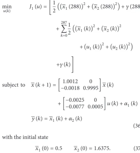
𝑢(𝑘) 𝐽1(𝑢) = [

1

2((𝑥1(288))2+ (𝑥2(288))2) + 𝛾 (288)

+287∑

𝑘=0

1

2((𝑥1(𝑘))

2_{+ (𝑥} 2(𝑘))2

+ (𝑢₁(𝑘))2+ (𝑢₂(𝑘))2)

+𝛾 (𝑘)]

subject to 𝑥 (𝑘 + 1) = [ 1.0012_{−0.0018 0.9995] 𝑥 (𝑘)}0

+ [−0.0025_{−0.0077 0.0005] 𝑢 (𝑘) + 𝛼}0 ₁(𝑘)

𝑦 (𝑘) = 𝑥1(𝑘) + 𝛼2(𝑘)

(36)

with the initial state

𝑥1(0) = 0.5 𝑥2(0) = 1.6375. (37)

By applying the algorithm proposed to solve Problem

(𝑀), the computation result is shown inTable 1. There is a

99.27 percent of reduction to the cost function, which gives the final cost 1.1810 units. The graphical results, which present the trajectories of output, state, and control, are shown,

respectively, in Figures1,2, and3. It is noticed that the model

output sequence tracks closely to the real output sequence

with the output residual 4.8 × 10−5. Both of the smooth

trajectories of state and control show the optimal expected solution to the original optimal control problem.

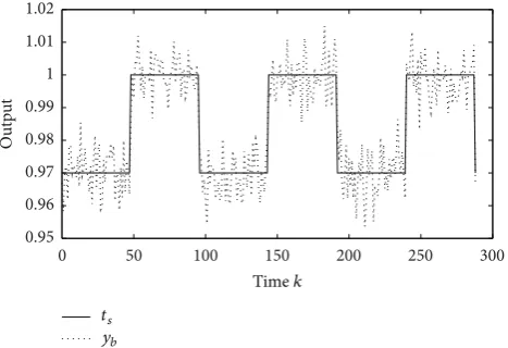
Now, consider the target sequence that is a periodic

square wave, with(0.97, 0.2)Tfor the first 48 time points and

(1.0, 0.1)T _{for the second time points, as discussed in [34].}

Let this target sequence be the real state sequence in Problem

(𝑃). Then, the real output sequence is measured and is fed

back into the parameter estimation problem. Here, the model

used in Problem (𝑀) remains the same as we mentioned

above.Figure 4shows the model output trajectory, which is

generated by the algorithm proposed, and tracks the target sequence accordingly.

(8)

0 50 100 150 200 250 300 0.25

0.3 0.35 0.4 0.45 0.5

Ou

tp

ut

y

yb

Timek

Figure 1: Output trajectories: real output𝑦(𝑘)and model output

𝑦(𝑘).

0 50 100 150 200 250 300

0.2 0.4 0.6 0.8 1 1.2 1.4 1.6 1.8

St

at

e

Timek

x1

x2

xb1

xb2

Figure 2: State trajectories: real state𝑥(𝑘)and model state𝑥(𝑘).

0 50 100 150 200 250 300

0 0.5 1 1.5 2 2.5

Co

nt

ro

l

Timek

−0.5

−1.5 −1

u1

[image:8.600.313.547.74.234.2]

u2

Figure 3: Control trajectories:𝑢₁(𝑘)and𝑢₂(𝑘).

6. Concluding Remarks

In this paper, a computational approach was proposed, where the efficient output solution of the discrete time nonlinear stochastic optimal control problem is obtained. In our approach, the model-based optimal control problem is simplified from the original optimal control problem, where the adjusted parameters are introduced into the model used. On this basis, the differences between the real system

0 50 100 150 200 250 300

0.95 0.96 0.97 0.98 0.99 1 1.01 1.02

Ou

tp

ut

Timek ts

yb

Figure 4: Output trajectories: target sequence 𝑡_𝑠(𝑘) and model output𝑦(𝑘).

and the model used are computed, and the integration of system optimization and parameter estimation could be made interactively. Establishment of the matching scheme by feeding back the output sequence that is measured from the real plant into the model used improves the accuracy of the model output sequence. For illustration, the wastewater treatment problem was studied, and the efficiency of the approach proposed is highly proven.

Conflict of Interests

The authors declare that there is no conflict of interests regarding the publication of this paper.

References

[1] A. Bagchi,Optimal Control of Stochastic Systems, Prentice-Hall, New York, NY, USA, 1993.

[2] N. U. Ahmed,Linear and Nonlinear Filtering for Scientists and Engineers, World Scientific Publishers, Singapore, 1999. [3] I. A. Adetunde and N. K. Oladejo, “Note on the investigation of

nonlinear stochastic control theory: its applications,” Interna-tional Journal of Modern Management Sciences, vol. 2, pp. 94– 111, 2013.

[4] P. R. Kumar and P. Varaiya, Stochastic Systems: Estimation, Identification, and Adaptive Control, Prentice Hall, Englewood Cliffs, NJ, USA, 1986.

[5] R. E. Kalman, “A new approach to linear filtering and prediction problems,”Journal of Basic Engineering, vol. 82, no. 1, pp. 35–45, 1960.

[6] R. E. Kalman, “Contributions to the theory of optimal control,”

Bolet´ın de la Sociedad Matem´atica Mexicana, vol. 5, pp. 102–119, 1960.

[7] R. E. Kalman and R. S. Bucy, “New results in linear filtering and prediction theory,”Journal of Basic Engineering, vol. 83, pp. 95– 108, 1961.

[image:8.600.57.284.269.417.2]

(9)

[9] S. Yin, X. Yang, and H. R. Karimi, “Data-driven adaptive observer for fault diagnosis,”Mathematical Problems in Engi-neering, vol. 2012, Article ID 832836, 21 pages, 2012.

[10] M. Zamani, A. Abate, and A. Girard, “Symbolic models for stochastic switched systems: a discretization and a discretiza-tion-free approach,” In press,http://arxiv.org/abs/1407.2730. [11] Y. Zhang, J. Yang, H. Xu, and K. L. Teo, “New results on practical

set stability of switched nonlinear systems,” inProceedings of the 3rd Australian Control Conference (AUCC ’13), pp. 164–168, Fremantle, Australia, November 2013.

[12] S. J. Moura, H. K. Fathy, D. S. Callaway, and J. L. Stein, “A stochastic optimal control approach for power management in plug-in hybrid electric vehicles,”IEEE Transactions on Control Systems Technology, vol. 19, no. 3, pp. 545–555, 2011.

[13] Y. Zhu, “Uncertain optimal control with application to a portfolio selection model,”Cybernetics and Systems, vol. 41, no. 7, pp. 535–547, 2010.

[14] J. L. Stein, “Application of stochastic optimal control to financial market debt crises,” CESifo Working Paper 2539, 2009. [15] Q. Meng, Z. Li, M. Wang, and X. Zhang, “Stochastic optimal

control models for the insurance company with bankruptcy return,”Applied Mathematics & Information Sciences, vol. 7, pp. 273–282, 2013.

[16] P. Devolder, M. B. Princep, and I. D. Fabian, “Stochastic optimal control of annuity contracts,”Insurance: Mathematics and Economics, vol. 33, no. 2, pp. 227–238, 2003.

[17] V. M. Zavala, “Stochastic optimal control model for natural gas networks,”Computers & Chemical Engineering, vol. 64, pp. 103– 113, 2014.

[18] M. Lagang, “Stochastic optimal control as a theory of brain-machine interface operation,”Neural Computation, vol. 25, no. 2, pp. 374–417, 2013.

[19] C. Nkundineza and C. W. S. To, “Stochastic optimal control of linear multi-degree-of-freedom systems under nonstationary random excitations,” inProceeding of the 24th Conference on Mechanical Vibration and Noise, vol. 1, pp. 1165–1174, 2012, paper no: DETC2012-70482.

[20] R. Loxton, Q. Lin, and K. L. Teo, “A stochastic fleet composition problem,”Computers and Operations Research, vol. 39, no. 12, pp. 3177–3184, 2012.

[21] Y. Yin, P. Shi, F. Liu, and K. L. Teo, “Robust fault detection for discrete-time stochastic systems with non-homogeneous jump processes,”IET Control Theory and Applications, vol. 8, no. 1, pp. 1–10, 2014.

[22] K. Kobayashi and K. Hiraishi, “Modeling and design of net-worked control systems using a stochastic switching systems approach,”IEEJ Transactions on Electrical and Electronic Engi-neering, vol. 9, no. 1, pp. 56–61, 2014.

[23] C. Jiang, K. L. Teo, R. Loxton, and G.-R. Duan, “A neighboring extremal solution for an optimal switched impulsive control problem,”Journal of Industrial and Management Optimization, vol. 8, no. 3, pp. 591–609, 2012.

[24] H. Xu and K. L. Teo, “Exponential stability with 𝐿₂-gain condition of nonlinear impulsive switched systems,” IEEE Transactions on Automatic Control, vol. 55, no. 10, pp. 2429– 2433, 2010.

[25] C. Aghayeva and Q. Abushov, “Stochastic optimal control problem for switching systems with controlled diffusion coef-ficients,” inProceedings of the World Congress on Engineering (WCE ’13), vol. 1, pp. 202–207, London, UK, July 2013.

[26] S. L. Kek, K. L. Teo, and A. A. M. Ismail, “An integrated optimal control algorithm for discrete-time nonlinear stochastic sys-tem,”International Journal of Control, vol. 83, no. 12, pp. 2536– 2545, 2010.

[27] S. L. Kek, K. L. Teo, and M. I. Abd Aziz, “Filtering solution of nonlinear stochastic optimal control problem in discrete-time with model-reality differences,”Numerical Algebra, Control and Optimization, vol. 2, no. 1, pp. 207–222, 2012.

[28] S. L. Kek, M. I. Abd Aziz, K. L. Teo, and A. Rohanin, “An iterative algorithm based on model-reality differences for discrete-time nonlinear stochastic optimal control problems,”Numerical Algebra, Control and Optimization, vol. 3, no. 1, pp. 109–125, 2013.

[29] A. E. Bryson and Y. C. Ho,Applied Optimal Control, Hemi-sphere, Washington, DC, USA, 1975.

[30] D. P. Bertsekas,Dynamic Programming and Optimal Control, vol. 1, Athena Scientific, Belmont, Mass, USA, 1995.

[31] F. L. Lewis and V. L. Syrmos,Optimal Control, John Wiley & Sons, New York, NY, USA, 2nd edition, 1995.

[32] D. Dochain and G. Bastin, “Adaptive identification and control algorithms for nonlinear bacterial growth systems,”Automatica, vol. 20, no. 5, pp. 621–634, 1984.

[33] J. C. Spall and J. A. Cristion, “Model-free control of nonlinear stochastic systems with discrete-time measurements,” IEEE Transactions on Automatic Control, vol. 43, no. 9, pp. 1198–1210, 1998.

(10)

Submit your manuscripts at

http://www.hindawi.com

Hindawi Publishing Corporation

http://www.hindawi.com Volume 2014

Mathematics

Journal of

http://www.hindawi.com Volume 2014 Mathematical Problems in Engineering

Hindawi Publishing Corporation http://www.hindawi.com

Differential Equations

International Journal of

Volume 2014

http://www.hindawi.com Volume 2014 Hindawi Publishing Corporationhttp://www.hindawi.com Volume 2014

Mathematical PhysicsAdvances in

Complex Analysis

Journal of

Optimization

Journal of

Combinatorics

International Journal of Hindawi Publishing Corporation

Journal of

Function Spaces

Abstract and Applied Analysis Hindawi Publishing Corporation

International Journal of Mathematics and Mathematical Sciences

The Scientific

World Journal

Discrete Dynamics in Nature and Society

http://www.hindawi.com Volume 2014 Hindawi Publishing Corporation

Discrete Mathematics

Journal of

http://www.hindawi.com Volume 2014 Hindawi Publishing Corporationhttp://www.hindawi.com Volume 2014