Adaptive Byte Compression and Decompression: A New Approach for Fractal Image Compression

(1)

Adaptive Byte Compression and Decompression: A New

Approach for Fractal Image Compression

Bhumika Gupta

Assistant Professor Computer Science Engg. Deptt.

G.B.Pant Engg. College Pauri Garhwal,Uttrakhand

Ashish Negi,

Ph.D Associate Professor

M.C.A. Deptt. G.B.Pant Engg. College Pauri Garhwal,Uttrakhand

ABSTRACT

This paper addresses the area of image compression as it is applicable to various fields of image processing. On the basis of evaluating and analyzing the current image compression techniques this paper presents the Adaptive byte compression and decompression technique an approach applied to fractal image compression. It also includes various benefits of using image compression techniques

Keywords

Fractal,Self-similarity,IteratedFunction System(IFS) Fractal image compressin.

1. INTRODUCTION TO IMAGE

COMPRESSION

Image compression can be defined as minimizing the size in bytes of a graphics file without degrading the quality of the image to an unacceptable level. This reduction allows more images to be stored in a given amount of memory space but the major benefit is the reduction of the time required for images to be sent over the Internet or downloaded from Web pages[1]. There are several different ways in which image files can be compressed like JPEG , GIF, PNG, fractals and wavelets.For Internet use, the two most common compressed graphic image formats are the JPEG format and the GIF format. The JPEG method is more often used for photographs, while the GIF method is commonly used for line art and other images in which geometric shapes are relatively simple[2]. Other method like fractals and wavelets offer higher compression ratios than the JPEG or GIF methods for some types of images. In near future PNG format will replace GIF format.

2. FRACTAL IMAGE COMPRESSION

The basic concept of fractal image compression is to use the characteristics of self similarity in an image Imagine a special type of photocopying machine that reduces the image to be copied by half and reproduces it three times on the copy (see fig.2.1). Now we will see that what is the result happens when we feed the output of this machine back as input. Fig. 2 shows several iterations of this process on several input images. We can observe that all the copies seem to converge to the same final image, the one in fig.2.2(c). Since the copying machine reduces the input image, any initial image placed on the copying machine will be reduced to a point as we repeatedly run the machine in fact, it is only the position and the orientation of the copies that determines what the final image looks like. The way the input image is transformed determines the final result when running the copy machine in a feedback loop. However we must

Except for this condition the transformation can have any form [12].

In practice, choosing transformations of the form

i i i

i

i i i

a b

e

x

W

y

c d

y

f





 



_

_



_{ }

 

 





 

is sufficient to generate interesting transformations called affine transformations of the plane. Each can skew, stretch, rotate, scale and translate an input image. A common feature of these transformations that run in a loop back mode is that for a given initial image each image is formed from a transformed (and reduced) copies of itself, and hence it must have detail at every scale. That is, the images are fractals[12].

Barnsley[12] suggested that perhaps storing images as collections of transformations could lead to image compression This is the implication of fractal image compression. The extra detail needed for decoding at larger sizes is generated automatically by the encoding transforms. However in some cases the detail is realistic at low magnification and this is a useful feature of the method. Magnification of the original shows pixilation, the dots that make up the image are clearly discernable.

This is because of the magnification produced. Standard image compression methods can be evaluated using their compression ratios , the ratio of the memory required to store an image as a collection of pixels and the memory require to store a representation of the image in compressed form. The compression ratio of fractal is easy to misunderstand since the image can be decoded at any scale. In practice it is important to either give the initial and decompressed image sizes or use the same sizes for a proper evaluation, because the decoded image is not exactly the same as the original. Such schemes are said to be lossy.

[image:1.595.313.537.660.734.2]

(2)

[image:2.595.312.514.68.472.2]

Figure 2.2: The first three copies generated on the copying machine Figure 2.1 [Y]

2.1 The Fractal Compression Consists of

Following Steps

In Fractal image compression the encoding step is computationally expensive. A large number of sequential searches through a list of domains (portions of the image) are carried out while trying to find out the best match for another image partition Fractal image compression process starts with giving an image as input then in next step the image is split in X x Y range and domain blocks after that we start with comparing the range with domain blocks then store similar blocks along with transformation applied after that similar blocks are constructed with pattern space hereby producing the fractal model from the pattern space and storing the result. The following steps for fractal image compression are show in fig.2.3.

2.2 The New Approach Adaptive Byte

Compression Algorithm

Fractal image compression is time consuming in encoding process but compression ratio is also very important factor. In my work the major emphasis is on compression ratio, the proposed new approach i.e. Adaptive byte compression algorithm will increase the compression ratio to very high extend.

The image format chosen to illustrate adaptive byte compression is that of .BMP and the program only supports black and white images The algorithm include Adaptive byte compression algorithm and Adative byte decompression algorithm.

Reading image

Spliting into XxY range and domain blocks

Comparing range with domain blocks

Storing most similar blocks along with transformations applied

Similar blocks constructing a pattern space

Producing a fractal model from the pattern space

Storing Fractal Model

(Compressed Image)

Figure 2.3: Steps of fractal image compression

3. ADAPTIVE BYTE COMPRESSION

ALGORITHM

[image:2.595.64.293.76.335.2]

(3)

4. ADAPTIVE BYTE DECOMPRESSION

ALGORITHM

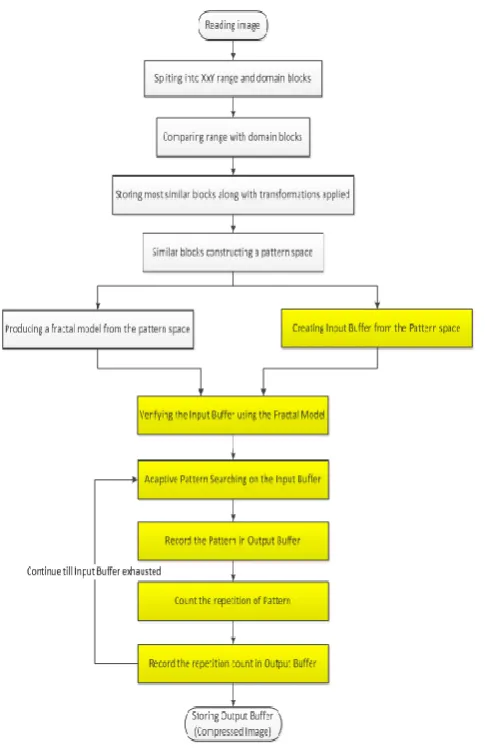
Adaptive byte decompression algorithm is applied on the .compressed file which is the final output of adaptive byte compression algorithm. This is unique algorithm which analyze the output buffer (.compressed file) and parse it. The output buffer consists of pattern and pattern repetition count. The algorithm picks the first pattern (i.e. simplest pattern is 0x00) and the count (followed by the pattern). It creates input buffer with the pattern at first location and the contiguous repetitions of pattern for the count specified. This phenomenon is repeated throughout the output buffer. Once completed for output buffer, the input buffer is created. The input buffer is called is .tmp file. The .tmp file is input for fractal decompression algorithm.The new approach applied to fractal compression algorith i.e adaptive byte compression algorithm showed in fig.3.1. consists of following steps-

Figure.3.1. Steps of Adaptive byte compression algorithm

5. COMPRESSION RATIO

The objective of image compression is to reduce irrelevance and redundancy of the image data in order to be able to store or transmit data in an efficient form. Compression ratio can be defined as the size of the compressed file compared to that of the

image size 100 image size

%

compressed

original

Fractal compression





original image size : 1 compressed image size

ratio

Fractal compression



Adaptive Fractal Compression % and Ratio is calculated by comparing the adaptive byte compressed image size with the original image size. The adaptive compression ratio provides the efficiency of adaptive byte compression algorithm.

Adaptive Fractal compression % 100 Adaptive byte compressed image size 100 original image size

   

  

 

Adaptive Fractal compression ratio original image size : 1

Adaptive byte compressed image size

 



   

[image:3.595.55.298.256.632.2]

6. TABLE OF RESULTS

Table 6.1. Size of original image

Original Image Size of Image/pixel

(width x Height)

Size of file in bytes

Signature1.bmp 512 x 512 32830 bytes

Portrait.bmp 550x382 27566bytes

horse.bmp 568x243 17558bytes

breeze.bmp 534x357 24338bytes

Table 6.2. Size of fractal compressed file

Original Image Size of .tmp file in bytes

Signature1.bmp 25194 bytes

(4)

Table 6.3. Size of adaptive fractal compressed file

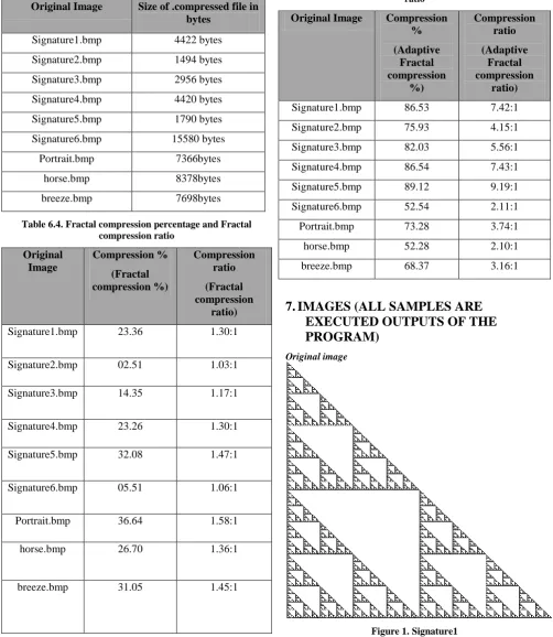
Original Image Size of .compressed file in bytes

Portrait.bmp 7366bytes

horse.bmp 8378bytes

[image:4.595.47.550.89.668.2]

breeze.bmp 7698bytes

Table 6.4. Fractal compression percentage and Fractal compression ratio

Original Image

Compression %

(Fractal compression %)

Compression ratio

(Fractal compression

ratio)

Signature1.bmp 23.36 1.30:1

Portrait.bmp 36.64 1.58:1

horse.bmp 26.70 1.36:1

breeze.bmp 31.05 1.45:1

Table 6.5. Adaptive Fractal compression percentage and ratio

Original Image Compression

%

(Adaptive Fractal compression

%)

Compression ratio

(Adaptive Fractal compression

ratio)

Portrait.bmp 73.28 3.74:1

horse.bmp 52.28 2.10:1

breeze.bmp 68.37 3.16:1

7. IMAGES (ALL SAMPLES ARE

EXECUTED OUTPUTS OF THE

PROGRAM)

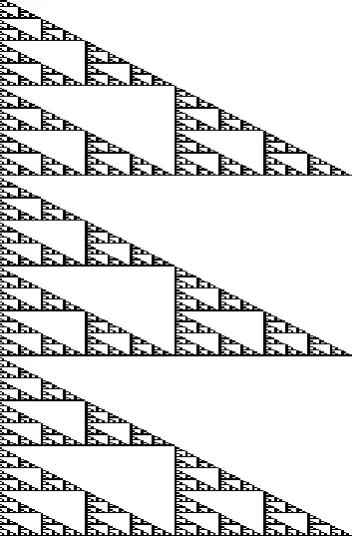
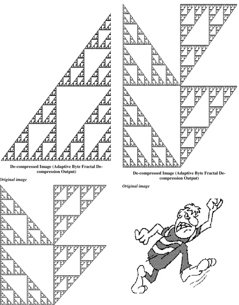
Original image

(5)

compressed Image (Adaptive Byte Fractal De-compression Output)

[image:5.595.55.286.72.307.2]

Original Image

Figure 2. Signature2

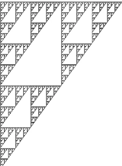
Original Image

[image:5.595.326.507.74.345.2]

(6)

[image:6.595.318.531.69.359.2]

Original image

Original Image

[image:6.595.84.265.70.396.2]

(7)

[image:7.595.55.547.64.690.2]

Original image

[image:7.595.307.543.71.407.2]

(8)

[image:8.595.59.535.58.739.2]

Original image

Figure 8. Horse

[image:8.595.69.261.315.720.2]

Original image

Figure 9. Breeze

De-compressed Image (Adaptive Byte Fractal De-compression

Output)

8. CONCLUSION

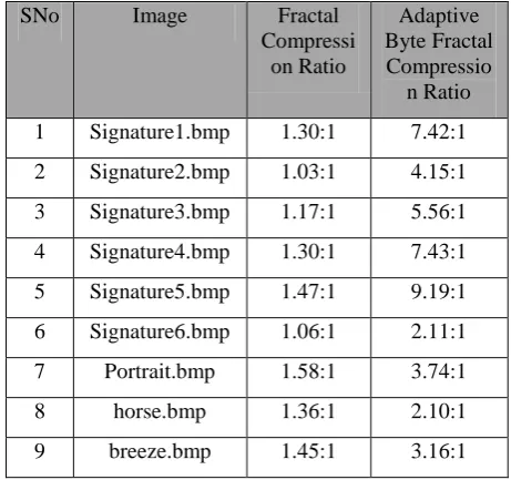
Table 8.1. Comparison table in terms compression ratio

SNo Image Fractal

Compressi on Ratio

Adaptive Byte Fractal Compressio

n Ratio

1 Signature1.bmp 1.30:1 7.42:1

7 Portrait.bmp 1.58:1 3.74:1

8 horse.bmp 1.36:1 2.10:1

[image:8.595.308.539.517.733.2]

(9)

Table8.2. Comparison table in terms compression percentage

S.No. Image Fractal

compression percentage Adaptive Fractal compression percentage

1 Signature1.bmp 23.36 86.53

7 Portrait.bmp 36.64 73.28

8 horse.bmp 26.70 52.28

9 breeze.bmp 31.05 68.37

The table8.1. shows the comparison of fractal compression ratio and adaptive byte fractal compression ratio. As we can clearly see from table 8.1. Compression ratio is enhanced multiple times as evident from results, with limited compromise with the compression time .But this can be eliminated with multi-threaded implementation of code and running on multi-tasking operating system, the compression time will not increase because in that case one thread will fill the fractal buffer and the second thread will do the adaptive compression.

The table8.2. indicates comparison in terms of compression percentage. It is clear from the table8.2 that the percentage of adaptive fractal compression is much higher than the percentage of fractal compression.

Now little highlight on decompression of image-  De-Compression time is minimally increased

 De-Compression results into original image or near to original image whose quality is same as fractal output.

9. REFERENCES

[1] Digital Image Processing by R. C. Gonzales and R. E. Woods, Addison-Wesley Publishing Company, 1992. [2] Two-Dimensional Signal and Image Processing by J. S.

Lim, Prentice Hall, 1990.

[3] Subramanya A, “Image Compression Technique,” Potentials IEEE, Vol. 20, Issue 1, pp 19-23, Feb-March ,2001.

[4] David Jeff Jackson & Sidney Joel Hannah, “Comparative Analysis of image CompressionTechniques,” System Theory 1993, Proceedings SSST’93, 25th Southeastern Symposium,pp 513-517, 7 –9March 1993.

[5] Hong Zhang, Xiaofei Zhang & Shun Cao, “ Analysis & Evaluation of Some Image Compression Techniques,” High Performance Computing in AsiaPacific Region, 2000 Proceedings, 4th Int. Conference,vol. 2, pp 799-803,14-17 May, 2000

[6] Ming Yang & Nikolaos Bourbakis ,“An Overview of Lossless Digital Image Compression Techniques,” Circuits & Systems, 2005 48th Midwest Symposium ,vol. 2 IEEE ,pp 1099-1102,7 – 10 Aug, 2005.

[7] scz-compress.sourceforge.net

[8] [8].M. Nelson, The Data Compression Book, San Mako, CA: M & T Publishing, Inc., 1992

[9] Lossless Data Compression, Report Concerning Space Data Systems Standards, CCSDS 120.0-G-2. Green Book. Issue 2. Washington, D.C.: CCSDS, December 2006.

[10]Gray, R. M. “Fundamentals of Data Compression”,International Conference on Information, Communications, and Signal Processing Singapore, September 1997. IEEE Publication, New York.

[11]Sayood, Khalid, Lossless Compression Handbook, Elsevier Science, San Diego, CA, 2003.

[12]Barnsley, M.F, Hurd, L.P, “Fractal Image Compression”, AK Peters, Wellesley, MA. (1993).

[13]Martin V Sewell, “Fractal Image Compression,” MSc Computing Science project report, 1994.