FORAGING ALGORITHM FOR OPTIMAL REACTIVE
POWER DISPATCH WITH VOLTAGE STABILITY AND
RELIABILITY ANALYSIS
1JAGANATHAN S, 2 Dr. PALANISAMY S.
1
Asstt Prof., Department of Electrical Engineering, RVS College of Engg & Tech,
2 Professor, Department of Electrical Engineering, Government college of Tech,
Coimbatore, Tamilnadu, India.
E-mail: [email protected], [email protected]
ABSTRACT
A novel bio-heuristic algorithm called Refined Bacterial Foraging Algorithm (RBFA) is proposed in the paper to solve the optimal power dispatch of deregulated electric power systems. The Optimal reactive power dispatch (OPD) problem has growing effect in modern electric power systems and the problem in need of to address the secure operation and optimal operation, with optimal location of FACTS devices, control of power flow based on stability indices and reliability analysis. So, this problem is well known as a multi-disciplinary and multi objective problem where in need of exact formulation and solution of the problem. The basic BFA is based on a metaphor of social interaction of E-coli bacteria the self adaptability of individuals in the group searching activities has attracted a great deal of interests in real word problems but it gives poor performance in global points when its applied to high dimensional and multi objective problems. To avoid the local optima and in order to track the good tracking ability of global solutions, the improved version of BFA algorithm is proposed and the proposed algorithm is called Refined Bacterial Foraging Algorithm (RBFA).The RBFA is improved version of the basic BFA with search direction phenomenon, variation of step sizes in chemotaxis behavior and variation of position updating process. The optimal dispatch problem consist of reactive power dispatch, optimal location of FACTS devices with transformer taps, real power loss and voltage stability margin are simultaneously optimized with effective controls and limits. The evaluation analysis of proposed work carried out with Standard IEEE systems. The simulation result shows the performance of RBFA is superior or comparable to that of the other algorithms and is greatly in terms of speed of convergence, optimization quality, robustness and fast convergence ability.
Keywords: Bacterial Foraging Algorithm, Refined Bacterial Foraging Algorithm, Multi-Objective
Optimization, FACTS Devices, Reactive Power Dispatch, Q-V Analysis, Stability Indices.
1. INTRODUCTION
The optimal dispatch of a power system is required to proceed the optimal planning of devices or facilities for the power system. The important roles of optimal power system operation are real and reactive power dispatch and maintain the voltage stability limit, but it’s directly connected with service quality and reliability of power system. However, the modern power system requires not only quality of supply and it’s strongly connected with needs of economy and security of the system. In order to address these requirements the optimal reactive power dispatch problem (OPD) proposed here and its improved version of optimal power flow (OPF) problem.
introduced is to address the OPD problem and single objective solution is not at all possible to solve the these type of issues, especially in multi-disciplinary problems [5] [6].
The simultaneously optimization not only consist of optimization and also satisfy the controls and limits related to optimization problem. The control strategies aim is to avoid some of the symptoms, voltage instability which lead to voltage collapse like heavy loading, transmission outages, or shortage of reactive power and the limits or constraints of OPD problem are real power generation, reactive power generation, bus voltages and settings of transformer taps with FACTS devices.
The increases of active power loss is affects the economy of the power systems and systems need to rescheduling for proper operation. The connection of above the reactive power loss leads to deviates the system voltage profile; finally it diminishes the reliability and stability of the system. So, the OPD problem is one of the most important and challenging problems in de-regulated environment and because, It is address to the optimal points of multi-objective functions of OPD problem as to determine the cost of operating, minimize the real power loss by Reactive power dispatch and it’s by optimal location of the Flexible AC Transmission Systems (FACTS) with minimum cost while keeping an adequate voltage profile. Hence, the system in need of proper co-ordination between FACTS devices and transformer taps and stability indices will leads the compensation requirements, voltage stability and co-ordination controls [10][15].
The OPF has long history, initially the Carpentier introduced a generalized optimization model of power system for solving OPF problem and this model comprises only an economic dispatch solution with nonlinear programming application. After the year, the Dommel and Tinney was introduced methodology to solve the optimal power flow method but this method spokes only fuel cost minimization as a single objective problem. The later the optimal operation of power system problem mainly focused on two major areas real power dispatch and other is reactive power dispatch problem. The literature clearly states all the solution techniques based on single objective problems [7] [21].
Initially, the conventional technique are usually used for solve the optimal problems but these techniques produce local optimum when the search space is irregular and overcome these demerits, many techniques are introduced such as, such as
gradient based search technique[21], the Newton’s method[21], interior point method[15] [18].But, the above mentioned techniques are failed, when finding the global solutions because solutions of these techniques are struck in local optima level and are needed well defined objective functions and constraints with derivative level. The development of evolutionary and other social intelligence techniques are plays major role in optimization problems, such as the computational intelligent techniques are Genetic Algorithm (GA) and Evolutionary Algorithm (EA) but GA has two major drawback’s one is ability to track the local optima and second one is premature convergence and the EA is not only premature convergence but also languish. The Social intelligence techniques also Ant Colony Optimization (ACO), Particle Swarm Optimization and Foraging Algorithm (BFA) are well suitable for multi-objective and complex problems [5] [6] [15] [16].
In the past decades, the real power dispatch and reactive power dispatch or OPF problems has a single objective function such as either fuel cost optimization or reactive power compensation. But, the optimal power flow problem or OPD problem was modified and satisfy constraints of modern power systems in de-regulated environment and also consists of multi-objective optimization. The simultaneous optimization is needed here for get exact solution of this problem comprise of above mentioned modules. Therefore, the new algorithm is developed and presented to solve OPD problem in multi-objective perspective and this problem consists of non linear objective functions and set of nonlinear functional equality constraints and inequality constraints. The main purpose of an OPD problem is mainly for voltage profile optimization via reactive power dispatch with effective control of FACTS devices and reliability analysis. The problem is formulated as a nonlinear constrained MOB problem where the real power loss and voltage stability objectives are optimized simultaneously [9]-[16].
the usable capacity of present, as well as new and upgraded of complex power system network. The proposed method can provide a good solution even the problem has many local optimum solutions at the beginning and computational implementation results involving IEEE standard test systems are given to demonstrate the validity of this method, and results are comparable with other technique. The proposed algorithm also identifies weak buses
and selects those buses as candidate buses for
installing new reactive power sources to enhance system security via stability indices and Q-V reliability analysis.
2. PROBLEM FORMULATION
In this work, the consideration FACTS device along with OPD problem is treated as optimization problem and it is formulated as a multi-objective optimization problem and this problem mainly focused on voltage profile optimization, week bus identification by proposed model, voltage stability and reliability analysis via stability indices and Q-V reliability analysis. The most of the researchers are not considering real power dispatch and total fuel cost while operating the reactive power dispatch optimization, but here the proposed approach is considering all the sub problems of OPD problem. Because the modern power system in need of optimize without omitting any parameters which is related to optimal operation of power system.
2.1 Objective Functions Real Power Loss (PL):
This objective is to minimize the real power loss in transmission lines that can be expressed as e :
PL= [ Vi2 + Vj2 – 2ViVj cos (δi – δj)]
(1)
Where Nl Is the number of transmission lines;
Gk is the conductance of the kth line; Vi <δi and
Vj<δj are the voltages at the end buses i and j of
the kth line respectively. Here, the cost optimization
also consider, while solving real power loss solution.
Active Power Losses:
g l
P=P P- ≥0 (2)
Where P is the total transmission active losses of
the power system in MW; Pg is the total active
power generated in MW and Pl is the total load of
the system in MW.
Average Voltage Deviation:
[
]
N
d i 1 act des
V =
∑
= V −V N (3)Where Vd is the per unit(pu) average voltage
difference; Vact is the actual voltage at bus bar i(pu)
and Vdes is the desired voltage at bus bar i (pu).
Maximum Voltage Deviation:
Vm =Max |Vact −Vdes|≥ 0 (4)
In summary, the optimization problem to be solved is the following
Minimize F= [ PL P Vd Vm ] (5)
Subject to equality and in-equality
constraints are given below.
2.2 Problem Constraints: Equality Constraints:
These constraints represent typical load flow equation as follows.
(
)
(
)
NB
Gi Di i j=1 j ij i j ij i j
P - P - V
∑
V G cos δ - δ + B sin δ - δ = 0(6)
(
)
(
)
NB
Gi Di i j=1 j ij i j ij i j
Q - Q - V
∑
V G sin δ -δ + B cos δ -δ = 0(7)
Where i=1….NB, NB is the number of buses; PGi
and QGi are the generator real and reactive power
respectively. PDi and QDi are the load real and
reactive power respectively Gij and Bij are the
transfer conductance and susceptance between bus i and bus j respectively.
Inequality Constraints:
These constraints represent the system operating constraints as follows.
Generation Constraints:
Generator power PGi , voltages VG and reactive
power output QG are restricted by their lower and
upper limits as follows:
PGimin ≤ PGi≤ PGimax , i=1,…., NG (8)
VGimin ≤ VGi≤ VGimax , i=1,…., NG(9)
QGi
min ≤ Q Gi≤ QGi
max
, i=1,…, NG (10) Where NG is number of generators.
Transformer Constraints:
Transformer tap T settings are bounded as follows:
Timin ≤ Ti ≤ Timax , i=1,…, NT (11)
Where NT is number of Transformers.
Switchable VAR sources Constraints:
Switchable VAR compensation QC is restricted
by their limits as follows:
QCimin ≤ QCi≤ QCimax , i=1… NC (12)
Load Bus Voltages:
These include the constraints of voltages at load
buses VL as follows:
VLimin ≤ VLi ≤ VLimax , i=1,…,NL (13)
3. RELIABILITY ANALYSIS FOR OF CRITICAL LINES AND BUSES
3.1 Voltage Stability Analysis and Fast Line Flow Index
To show the effectiveness of proposed approach formulated and it’s used to solve the voltage profile optimization and check the load ability of system subjected to power flow equations under various operating conditions. The proposed method gives better Voltage profile when installing the FACTS devices [15] under various operating conditions and the quality of solution based on better Voltage magnitude irrespective of operating conditions. So the proposed method enhances better voltage profile optimization via reliability analysis.
The Fast Line Flow Index (FLFI) method is to ensure the power flow control and stability index between the receiving and sending end power in the intercommoned power system network. In this method the set of power flow equations is to co-ordinate the real and reactive power flow control over a transmission line in both the directions of flow. The set of equations were used to analysis and identification of critical lines and weak buses.
The maximum voltage deviations are pointed out in the particular systems in the view of voltage stability analysis [10].the analysis of line flow approach is given for two bus system
(
)
24 ( sin
fl j i
L = XQ V θ δ−
(14)
fl
L - Fast Line Flow Index
Θ- Angle in the impedance angle from impedance triangle
δ- Influence of the vector diagram, angle between sending end and receiving end voltage.
X-line reactance
Qj - reactive power flow at the receiving
end
Vi – sending end voltage
3.2 Voltage Stability Approach (VSA)
The Voltage Stability Approach (VSA) is comprises a Voltage Stability Index (VSI) against voltage collapse and line stability based on concept of maximum power transferred through a transmission line flow. The optimal location and control variables of FACTS devices are based on
voltage stability index of each transmission line.The loading of real or reactive powers are leads to identify the critical transmission paths and via weak buses.
A voltage stability index is deals the maximum voltage deviation via power flow in transmission, which is leads to maintain the voltage profile against loading condition. Therefore Voltage Stability Approach is gives the corrected voltage drop of a line segment is defined as the projection of the receiving end bus voltage of that segment on the voltage phasor of the generator which is the starting point of that transmission path. This index is given by
act
VSA
=
hV
− ∆
V
(15)Where Vact is actual generator voltage, h is
parameter for correct the desired constant value and ΔV is sum of corrected voltage drops by the side of a transmission path. The real Power and Reactive Power flow in Transmission line is defined as a sequence of connected buses with declining voltage magnitudes again starting from a generator bus.
The FLFI and VSA are analysis to carry out the real and reactive power loading and with address of critical lines and weak buses. The voltage deviation and voltage stability enhancement is happen for placing of FACTS devices. The optimal location FACTS devices, Voltage control via reactive power support, the reliability analysis is carried out via Stability indices. Further Q-V analysis is deals of Voltage stability analysis and Reactive power compensation design in FACTS devices.
3.3 Q-V Analysis: Reactive Power Control and Voltage Stability Index
Q-V analysis encompass of voltage stability analysis, reactive power control variables and VAR compensation design is given below the matrix
P PV
Q QV
J
J
P
J
J
v
Q
δ
δ
∆δ
∆
=
∆
∆
Where
P
∆
and∆
Q
are incremental real, reactive power.∆δ
and∆
v
are incremental bus voltages and busangles
P
J
δJ
PVJ
QVandJ
Qδare sub matrixes ofjacobian in power flow equation.
by taking necessity actions. This analysis gives a detail view of stability enhancement by modifications and rescheduling of control variables like real and reactive power controls.
Power flow equations after the increments in bus voltage magnitude and angel, real and reactive power are can be written as follows.
1
2
3
4
J
J
P
J
J
v
Q
∆δ
∆
=
∆
∆
(16)OR
P PV
Q QV
J
J
P
J
J
v
Q
δ
δ
∆δ
∆
=
∆
∆
The stability point of view, according to point of operation keeping real power constant is. The incremental relationship of Q-V analysis is given below.
[ ] [ ] [ ]
1R
V
J
−Q
∆
=
∆
(17)
where JR is known as reduced Jacobian and is
given as follows.
1
R QV Q PV P
J
=
J
−
J
δJ
−J
δ(18) The voltage stability analysis is further with help of sub matrix jacobian is given in the following equation
.
k dk
k kk k
k k
Q
q
L
B
V
V
V
∂
=
= −
−
∂
(19)Where,
dk
q
Reactive power demand at nth busk
L
Voltage stability index at nth buskk
B
Imaginary part of Admittance matrixUsing the reduced Jacobian matrix, the sensitivity of Voltage stability index with respect to
VAR injection at kth bus can be written as
k
k
Q VSI V
V ∂
= ∆
∂ (20)
Where
[ ]
1R inj
V J − Q
∆ = ∆
(21) Voltage stability index depends upon the following parameters voltage profile improvement,
reactive power demand, voltage at Kth bus and
connectivity of the bus, i.e. Bkk Generally
the product BkkVk is important and dominant. If
Bkk is large then relatively lesser voltage magnitude
may be sufficient to give required voltage stability margin.
1
NC f
k k kj k
k
L
L
A
C
=
≈
+ ∑
∆
(22)
Where
∆
C
k is kth bus change in reactive powercontrol variables.
NC is total number of reactive power control variables which includes PV buses, Tap changers and switchable shunt reactors.
Akj is the sensitivity coefficient of VSI with
respect to the change in reactive power control variables. In order to improve the Voltage stability and maintain the voltage profile end results of Q-V analysis; it is required to inject reactive power at the critical and weak buses
3.4 Proposed Strategy for Placement of Facts Devices
The result stability indices are to address to the optimal location of FACTS devices in addition to this the RBFA algorithm requires particle representation. Thus because of any optimization problem is need of parameters optimization of the optimization problem and the OPD problem also consists of many parameters. Since the goal of optimization was to allocate the FACTS devices, with optimal value of all the parameters and effective controls. A particle is represented with the following strings of variables control.
Z = [Pgi….Pg N Qgi……..QgN Vgi...VgN, VLi...VLN
Qci……..QcN ]
Where
Vgi,VLi = the voltage magnitude of generator
bus.
Pgi = the active power generations at bus i.
Qgi, Qci = the reactive powers and reactive
power compensation devices.
FACTS devices = Weak bus identification and
status of installing FACTS devices
Xij=XT.line+XTCSC (23)
Qi= QSVC
(24)
XT.line = reactance of transmission line
4. BACTERIAL FORAGING ALGORITHMS
swarming. Reproduction comes from the concept of natural selection and only the bacteria best adapted to their environment tend to survive and transmit their genetic characters to succeeding generations while those less adapted tend to be eliminated. Elimination – dispersal event selects parts of the bacteria to diminish and disperse into random position in the environment, which ensure the diversity of the species. [1] [7]
4.1 Chemotaxis
This is process achieved through swimming and tumbling by flagella. Depending upon the rotation of flagella in each bacterium decides it’s pattern, whether it should move in a predefined direction as swimming or altogether in different directions as tumbling in the entire lifetime. The entire lifetime bacteria are set to two mode operation; these modes enable the bacteria to move in the random directions. An E-coli bacterium can move in two different ways alternatively: tumble and run. A tumble is represented by a unit walk with random direction, a unit walk with the same direction as the previous step indicates a run. A chemotactic process is started by one step of tumble and followed by uncertain steps of run, depending on the variation of the environment.
In a tumble, the position of the ith
bacterium is updated as:
(
) ( ) ( )
i( j 1, k, l) i j, k, l C i ‹ j
θ + = θ + Φ (25)
Where θI (j,k,l) is the position of the ith
bacterium at the jth chemotactic step of the kth
reproduction loop in the lth elimination-dispersal
event, C(i) is the size of the step taken in the
random direction specified by the tumble,<Φ(j) is
the angle of the direction which is randomly generated in the range of (0,2π).The fitness value of
the ith bacterium at θi(j,k,l) is represented by
ji(j,k,l).If θi(j+1,k,l) the cost is better it means lower
then at θi(j,k,l). Now the next step of step size of
C(i) in this same direction will be taken and once again, if the step resulted in a position with the better cost the previous step means another step taken. This swim is continued as long as it continuous to reduce the cost and its depending upon maximum number of steps, Ns. The Nc is number of chemotaxis steps.
4.2 Swarming
During the process, the E-coli bacterium produces attraction convergence characteristics and has to desire when anyone bacteria reaches the best position or location, it should attract other bacteria. So, that they converge in that location and this will happen by generation of attraction signal and also
in the meantime, each bacterium releases repellent to warn other bacteria to keep a safe distance from. The E-coli bacterium has own in is, a specific sensing, cell to cell signalling, actuation and decision-making mechanism and because of these properties is lead to provide global search . BFA simulates this social behavior by representing the cell to cell signaling
(
) (
)
(
, , , , ,)
(
,(
, ,)
)
1
= ∑ =
i s i i
j j k l j k l jcc j k l i
θ
θ
θ θ
α
2 exp
1 1
∑ ∑
= s= −d −w p= − i
attract attract m m
i m θ θ
2 exp
1 1
∑ ∑
+ s= h −w p= − i
m m repellant repellant
i m θ θ
(26)
Where
dattract - depth of the attractant effect
ωattract - measure of the width of the attractant
hrepellant = dattract - height of the repellent effect
ωrepellant - measure of the width of the repellent
P-number of parameters to be optimized S-number of bacteria
Where θi=[θ1,θ2,…….., θp]T is a point
optimization domain and it’s the location of the ith
bacterium on the P-dimensional optimization
domain,θi
m is the mth component of ith bacterium
position, θ={θi
li=1,2,….,S} represents the position of each member in the population of the S bacteria, θi
m is the mth component of θI, θim is the mth
component of position θt
for the tth bacterium, d
attract is a quantification of how much attractant is
released, ωattract is a measure of the diffusion rate of
the chemical signal, h repellant and ωrepellant are the
magnitude and width of the repelling effect
respectively, Jicc(θ,θi(j,k,l)) indicates the signals
released by the ith bacterium and Jcc(θ
i, θ) is
time-varying function. Jcc(θi,θ) represents the combined
attraction and repelling effects received by the ith
bacterium.
4.3 Reproduction
After Nc chemotactic steps, a reproduction
step is taken. Assume that, Nre is the number of
reproduction steps is taken. The final population of bacteria undergoes the reproduction process and here, the least healthy bacteria die and other healthiest bacteria split into two at the same location. All the bacteria are sorted according to
their fitness Sr (Sr=S/2, for convenience S is
assumed to be a positive even integer) and the step
bacterium in the chemotactic loop are accumulated and calculated by:
N Ji(j,k,l) j 1c
∑ =
i N 1
jH Ji(j,k,l)
j 1c+
= ∑ = (27)
Where jiH represents the health of the ith
bacterium.
For simplification the number of the bacteria keeps constant in each chemotaxis process. The characters including location and step length of the mother bacterium all reproduced to the children bacteria. Through this selection process the
remaining Sr unhealthier bacteria are eliminated
and discarded.
4.4 Elimination-Dispersal
The process of chemotaxis and reproduction are not enough for finding global solutions and to improving process of global search ability, the
elimination-dispersal event introduced after Nre
steps of reproduction. This elimination-dispersal event helps the bacterium avoid being trapped into local optima and dispersal events may place bacteria near global solutions and also the behavior of bacteria seeks out in favorable environments. The bacteria are eliminated and dispersed to random positions in the optimization domain
according to the probability, ped and the number of
the event is denoted as Ned.
4.5 Refined Bacterial Foraging Algorithm
The survival of species in any natural evolutionary process depends upon their fitness criteria, which relies upon their food searching and motile behavior. The law of evolution supports those species who have better food searching ability and either eliminates or reshapes those with poor search ability. The genes of those species who are stronger are propagated in the evolution chain since they posses ability to reproduce even better species in future generations. So a clear understanding and modeling of foraging behavior in any of the evolutionary species, leads to attempts better solution for any optimization. So, this is way here proposed the new algorithm.
The basic foraging algorithm consists of four steps are Chemotaxis, swarming, reproduction, elimination and dispersal. Chemotaxis is the activity that bacteria gathering to nutrient-rich areas spontaneously. A cell-to-cell communication mechanism is established to simulate the biological behavior of bacteria swarming. Reproduction comes from the concept of natural selection and only the bacteria best adapted to their environment tend to survive and transmit their genetic characters
to succeeding generations while those less adapted tend to be eliminated. Elimination –dispersal event selects parts of the bacteria to diminish and disperse
into random position in the environment. The
proposed method based on foraging behavior of bacteria and some modifications is made through from basic foraging algorithm. The modified algorithm named as Refined Bacterial Foraging Algorithm (RBFA) and RBFA is proposed in this paper. The performance of basic foraging algorithms is well suitable in single objective problems and static environments and step length of the basic BFA is a constant parameter which may guarantee good searching results for small optimization problems. However it is applied to multiple objectives, dynamic environments and high dimensional problems it’s gives poor performance and convergence characteristics also not good and many times it trapped into local optima solutions. The process of search direction and step length is important in multiple objectives and dynamic environments. The proposed approach made some modification in step length; Chemotaxis behavior and adding velocity vector for improve speed of convergence and attaining global solution and also suitable diversity for global search and its improves speed of convergence.
4.6 Search Direction And Chemotaxis Process: The Chemotaxis behavior is modelled by a tumble-run process that consists of a tumble step and several run steps. The tumble run process follows gradient searching principles, which means the bacteria’s position is updated in the run steps by the gradient information provided by the tumble step. In each bacteria step size, unit length, dimension and random direction coordination are
much important, a search direction Wid (j) and a
step length Lid (j) are calculated separately for each
bacteria i, on each dimension d for each time step
or tumble-run process or iteration j, Wid (j) =1
means the i-th bacteria goes towards the positive direction of the coordinate axis on the dimension d, its indicates the follow tumble process and
consecutive run process. Wid (j) = -1 means the
bacteria goes towards the negative direction, its
follow again tumble process and Wid (j) =0 means
the bacteria stays at the current position; it means the bacteria reaches more nutrient position.
When any one of b
acteria finds best
position, it
should attract other bacteria so that they converge in that location. The Figure.1 and Figure.2 shows the difference of random direction and after the search dimension estimation, there isdirection estimation leads to finding the distance of best bacteria from rest of others and the process convergence time minimized. While the distance known, it’s easy to attain the swarming process for
new Chemotaxis stage. The current position ith the
bacterium, in d dimensional search space and jth
tumble-run process is updated
(
)
( )
( )
( )
id id id id
X j+ =1 X j +L j W j (28)
Once the direction and angle is decided by the tumble step, to reach the position it takes several steps (until the position of worst). The rotation angle Ф is related to the number of the dimensions, the number dimensions desired by objectives.
1 round d
π
φ
=+ (29)
Where, d- search dimension and πis the number of
dimensions.
4.7 Position Updating Process
In this process the step size calculation are initiated with help of position updating process. The basic methodology is adopted in BFA, In order to meet these criteria. The E-coli cells provides attraction signal to each other, so that they swarm or swim together and towards to the best location and swarming pattern based on cell-to-cell communication. But in this process shows slow converge only and in order to improve this process, the velocity factor added with other bacteria so as to reach best bacteria position and this velocity vector added according to other bacteria position. The Figure.3 and Figure.4 shows strength of RBFA algorithm with help of velocity factor and attraction factor leads to converge the bacteria in global position. The position updating process mainly focus on best bacteria and each dimension is given by
( )
(
)
Xid j =α Xid best−Xid (30)
Where α is a factor to desire the strength of the bacterium’s attraction factor for improving the strength of the bacterium’s attraction towards to the
best position and for faster convergence., Xbest
indicates the position of current best global solution updated after each function evaluation, and Xi is
the position of the ith bacterium at the jth iteration
after the tumble run process.
Fig.1. Initial Search With Random Directions
Fig.2. Modification Of Chemotaxis Behavior In Run Process With Help Of Search Direction And Search
Dimension
If a anyone bacteria reaches better position in order to direct the other bacteria to best position, the attraction signal is not enough to reach the best position. Therefore, in order to attract other bacteria and also obtain the bacteria position by using equation
(
)
(
)
Xid j+ =1 α Xid best−Xid +Vj (31)
Fig.4. Communicating To Other Bacteria
Fig.5. Reaching Global Point With Help Of Position Updating Process
So, in the process the velocity factor Vj is
binding with position updating process and also is pilot to determine the best position according to the previous best positions. Update best bacteria position and add the velocity according to reach the best position, the velocity factor desired by depending upon according to position of best and
other bacteria. The velocity factor Vj also gives
direction to global best value or its used to identify global best value.
4.8 Step length
The basic BFA shows a step size is a constant parameter and it’s suitable to finding the solution in single and small optimization problems. However, when applied to multiple objective problems and dynamic environmental problems it shows poor
performance. The basic BFA with fixed step size is
failure in reaching the optimal point for the following reasons. The first case, if step size is very high then the accuracy gets low although the bacterium reaches the locality of optimum point quickly and it moves around the maxima for the remaining chemotactic steps. The second case, if the step size is very small, it takes many chemotactic steps to reach the optimum point and its lead to slow convergence and rate of
convergence decreases. Meanwhile to reach the optimal point it takes convergence time and number of iterations increases. So, in order to reach the optimal point, speed of convergence and search
ability the controlling of step length is essential. In
this paper the proposed RBFA following consideration in determining step length process with help of search dimensions, If deviation is very high then the step size must be increased and if the deviation is small in which case the bacterium is close to the optimum point the step size is to be reduced and also improve the performance the swim walk considered instead of the constant step. The Figure.5 shows effect of best fitness of solution and reaching the global point with minimum of time.
For a each bacteria, the location of the ith bacterium at the jth chemotactic step, rth
reproduction step and l th elimination / dispersal
event is represented by Xid(j,k,l)∈ ℜ
p
. After a tumble, the location of the ith bacterium is represented by
(
1, ,)
(
, ,)
L i,( ) ( )
id id
X j+ r l =X j r l + j φ j (32)
Where L i,
( )
j =Lid( )
j Wid( )
jThe J(i,j,k,l) is cost function of corresponding Xid (j,k,l).The fitness value of the ith bacterium at
Xid(j,k,l) is represented by jid (j,k,l). In this paper
the minimum fitness value jmin is defined as the
global optimum.
In a run, consecutive steps of size L(i,j) is the same direction as the tumble is taken, in condition
Xid (j+1,k,l) the cost function J (i,j+1, k,l) is better
(lower) than J(i,j,k,l). In this condition, the fitness
value of the ith bacterium in the rth step of the run
Ns indicates the maximum number of steps in a run
and also r is smaller than Ns. This swimming
operation is repeated as long as a lower cost is obtained until a maximum preset number of steps,
Ns, is reached.
In BFA the step length L is a constant and it
ensures accuracy and speed of the search. The size of the step length is dynamically adjusted in the reproduction and elimination-dispersal process, which ensures the bacteria moving towards the global optimum quickly at the beginning, and converging to the global optimum accurately in the
end. So the ith bacteria in dth dimension search
space the step length controlling vector is given by
( )
{
(
( )
)
}
L id =min L id −µ , n (33)
Where
is desired by according to position updating process and Chemotaxis process.
4.8 Multi- Objective Optimization
Multi-objective Optimization (MOO) problems
are defined as those problems "where two or
more, sometimes competing and/or incommensurable, objective functions have to be minimized simultaneously". In general, for a problem with n objective functions, the multi-objective formulation can be as follows
Minimize/maximize fi(x) for i=1, 2, 3...n
Subject to
Gj(x) ≤0 j=1, 2...J (34)
Hk(x) =0 k=1, 2...K
(35)
Often the multi-objective is combined into a single objective so that optimization and mathematical methods can be used. There are n objectives and p variables so f(x) is an n dimensional vector and x is a p dimensional vector corresponding to p decisions or variables, solutions to a multi-objective optimization problem are often mathematically expressed in terms of non-dominated or superior points.
4.9 Load Flow Solution
Whenever the operating conditions changes the electric power system in need of power flow optimization. So, it is necessary to solve the load flow problem numerous times. The RBFA based OPF problem requires, first define the behavior of bacteria initially for initialization of control variables for secure operation and next find the optimal solution with help of Foraging and swimming of bacteria and the bacteria size is to beset according to the updating process. The algorithm able to find optimal solution subject to load flow convergence and objectives function of cost function both smooth and non-smooth functions. The load flow is solved using a RBFA-based load flow developed using incorporating a Jacobian acceleration stage. In order to keep computation time to a minimum during the optimization, the step length is very much important and search direction and dimension for the load flow is dynamically adjusted according to the proposed algorithm.
Many OPF solution techniques handle generation node reactive power limits through the use of penalty functions exclusively. This can lead to convergence problems due to distortion of the solution surface, or in some instances, it may be necessary to switch a node in order to obtain a load-flow solution. The reactive power limits on all PV nodes other than the slack node and switching to a
PQ node are important in control of voltage. The above all the requirements are satisfied by solving the OPD problem by using the Load Flow solution.
4.10. Computational Algorithm and PSEUDO Code of RBFA
The multi objective Optimal Power Dispatch based on multi-objective optimization problem is can be solved by using Refined BFA. Read system data, here the standard IEEE30 bus system data [20] is considered. It contains load data, line data and generator data [20] [18] with cost coefficients.
Randomly initialize the position of each bacterium in the domain, set the position and fitness value of the best bacterium. Initialize the
parameters: S, p, Nc, NS, Nre, Nc, Ped, L (id), α, μ,
Vj, and n.
Randomly initialize the position of each
bacterium in the domain, set the position and
fitness value of the best bacterium as Xidb(j,k,l)
and jmin (j, k, l) respectively.
FOR (each bacterium i=1: S)
FOR (chemotactic loop j=1: Nc)
FOR (dimensions=1: π)
FOR (reproduction loop k=1: Nre)
FOR (elimination-dispersal loop l=1: Ned)
Evaluate the cost function J(i,j,k,l) Let Jlast = J(i,j,k,l) so that a lower cost could be
found Calculate Ji (j, k, l) and set it as Jlast;
Tumble:
Search direction identified with help of identification process according to RBFA
For bacterium I, set Ji(j,r) as Jlast. A random
vector ∆(i), with each element ∆m(i), m=1,2….. p,
a random number in the range [-1,1]. Move:
Move to a random direction
' ∆
∆× ∆
by a
unit walk, the new position is calculated by equation and start another chemotactic step.
Compute J(I,j+1,k,l) and use to compute
Jcc (θ, P (j+1,k,l)) then use to find the new
J(i,j+1,k,l).
Swim: let m = 0 (counter for swim length)
While m< Ns (no climbing down too long)
Let m=m+1
If J(I,j+1,k,l)<Jlast let Jlast = J(I,j+1,k,l) then take another step in the same direction and compute the new J(I,j+1,k,l).
Swim:
Update Xid(j+1, k, l).
IF (Jcurrent< Jlast)
WHILE (Jir+1(j+1, k, l)<Jir(j+1, k, l)
and r<Ns)
Set Jir (j+1, k, l) as jlast;
Run:
Update Xid(j+1, k, l)
Set new Jir+1(j+1, k, l) as
Jcurrent;
Swim:
Update Xid(j+1, k, l)
Recalculate Jir+1(j+1, k, l);
END WHILE END IF
END FOR (bacterium)
Calculate Jmin (j+1, k, l)
END FOR (chemotaxis) Sum:
Evaluate the sum of the fitness value Jihealth
for the ith bacterium.
Sort:
Sort bacteria according to their health Jihealth in ascending order.
Split:
The bacteria with the highest Jihealth values,
computed by die while the other Sr with the lowest
values split and take the same location of their parents.Eliminate other then health bacteria are to be eliminated.
Update:
Update the step length L (i,j). END FOR (reproduction) Disperse:
Disperse certain bacteria to random places
in the optimization domain with probability Ped.
Update:
Update the step length L (id) END FOR (elimination-dispersal) END
If it’s optimal solution is achieved means, the program will stopped
5. RESULTS AND DISCUSSIONS
To evaluate the performance of the proposed method based multi-objective optimal power dispatch problem with considering different IEEE standard systems.
From the year 1994 to now, the evolutionary and social behavior algorithms were dominating the algorithm in the field of optimization and especially in the power system problems. These algorithms are most powerful and population based heuristic algorithms, and these algorithms have been successfully applied to solve the multi-objective based optimal power dispatch problems [5] [5]
[17]. So, the proposed technique results are compared with other social behavior algorithms. The other algorithms are like Ant Colony Algorithm (ACO) with reactive power planning problems was analyzed in [5],it gives better results when the problem is simple but increase the complexity of problem like adding FACTS devices, voltage and line flow stability and it shows slower convergence. The Particle Swarm Optimization (PSO) and modified PSO were proposed in various optimization problems [23]. Considering the PSO, the attaining results were good but when solving the multi-modal and multi-objective functions, the PSO and modified version of PSO easily trapped in local solution but solving identification of parameters are very complex, like learning rate and velocity, so it becomes complex process. The basic Bacterial Foraging Algorithm (BFA) were analyzed with the problem of multi-objective based Transmission expansion planning problem in [7].The performance of BFA is better but step length is constant rate only. So, it’s not suitable dynamic environments like power system problems. The Modified version of Bacterial Foraging Algorithm (MBFA) was considered in [6], for analysis of optimal power dispatch problem with considering FACTS devices. The performance of attraction and repellant factor is not so better and the end result shows the process is time consuming process. Finally, the proposed algorithm RBFA were tested with different multimodal functions and are listed in [2] and the performance of proposed technique compared with other technique like ACO, BFA and MBFA algorithms [2].
5.1 Case Studies and Discussions
This section deals effectiveness of proposed approach, tested with using IEEE 6-bus, IEEE 9, IEEE 30 bus, New England IEEE 39 bus system and considering FACTS devices, stability indices analysis and Q-V analysis for multi-objective based optimal power dispatch problem. The load flow analysis is carried out with Newton-Raphson method incorporating jacobian analysis and the proposed method tested with considering and without considering FACTS devices. The support of FLFI and VSA analysis the identification of real and reactive power loading are controlled by Q-V analysis after the address of critical lines and weak buses.
5.2 IEEE 30-bus system
with off-nominal tap ratio in lines 6-9,6-10,4-12,27-2 and 9 buses of compensations 10, 16-9,6-10,4-12,27-2, 15, 17, 6-9,6-10,4-12,27-20, 21, 23, 24 and 29. The load data, line data, generator data are obtained from [18] [20]. The lower voltage magnitude limits at all buses are 0.95 pu and the upper limits 1.1 pu for the generator buses 2,5,8,11 and 13,and 1.05 pu for the remaining buses including the swing bus 1.The lower limits and the upper limits of the transformer tap settings are 0.9 and 1.1 pu respectively. The proposed algorithms and all other algorithms are executed with help of simulation software MATLAB. The programs were coded with MATLAB 7.0 software package and executed via Pentium-IV Computer.
Table 1 Comparison Of Results.
Variable BFA MBFA ACO
Proposed method
Total generation
(MW)
292.84 295.03 292.86 292.91
Fuel cost
($/h) 802.62 802.37 802.30
801.842
Losses
(MW) 9.759 8.424 9.427 8.267
Simulation
time (sec) 32.4 26.07 27.16 19.95
No. of.
Iterations 41 32 36 23
The objective of real power loss, reactive power compensation, voltage profile optimization and optimal location of FACTS devices with line flow, real and reactive power limits and tap setting values and results are tabulated in Table.1 and it shows the transmission losses greatly reduced and is comparable with similar social behavior algorithms. The total simulation time considerably reduced in MBFA and its compared to ACO and also basic BFO, but proposed method shows good organization in all the level because time consuming for convergence is very less even if consider multi-objective problem. The voltage stability limit is incorporated to improve the voltage stability in the various operating condition with impact of stability indices are good. The results of FLFI and VSA approaches is given in Table.2
Table 2. Results Of FLFI, VSA Approaches And Q-V Analysis.
SSC Bus Vssc in p.u Angle in
degree Qsh in p.u
30 1.0020 -18.0321 -0.0202
26 1.0014 -16.7872 -0.0137
Table 3. Results Voltage Magnitude For IEEE 30 Bus System
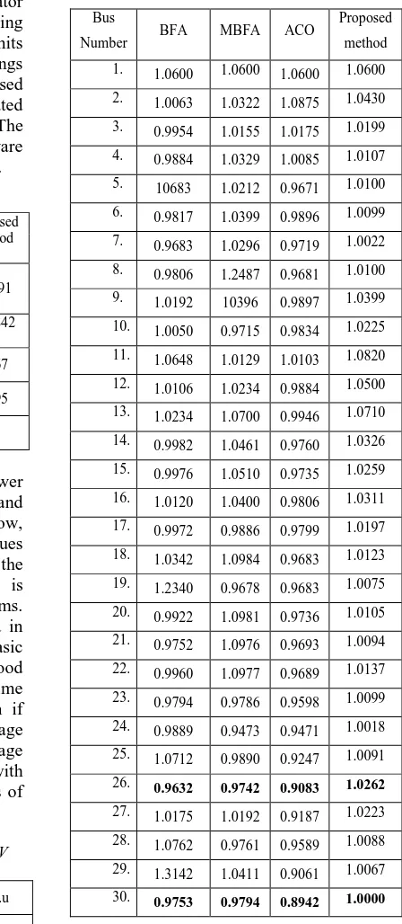
Bus
Number BFA MBFA ACO
Proposed
method
1. 1.0600 1.0600 1.0600 1.0600
2. 1.0063 1.0322 1.0875 1.0430
3. 0.9954 1.0155 1.0175 1.0199
4. 0.9884 1.0329 1.0085 1.0107
5. 10683 1.0212 0.9671 1.0100
6. 0.9817 1.0399 0.9896 1.0099
7. 0.9683 1.0296 0.9719 1.0022
8. 0.9806 1.2487 0.9681 1.0100
9. 1.0192 10396 0.9897 1.0399
10. 1.0050 0.9715 0.9834 1.0225
11. 1.0648 1.0129 1.0103 1.0820
12. 1.0106 1.0234 0.9884 1.0500
13. 1.0234 1.0700 0.9946 1.0710
14. 0.9982 1.0461 0.9760 1.0326
15. 0.9976 1.0510 0.9735 1.0259
16. 1.0120 1.0400 0.9806 1.0311
17. 0.9972 0.9886 0.9799 1.0197
18. 1.0342 1.0984 0.9683 1.0123
19. 1.2340 0.9678 0.9683 1.0075
20. 0.9922 1.0981 0.9736 1.0105
21. 0.9752 1.0976 0.9693 1.0094
22. 0.9960 1.0977 0.9689 1.0137
23. 0.9794 0.9786 0.9598 1.0099
24. 0.9889 0.9473 0.9471 1.0018
25. 1.0712 0.9890 0.9247 1.0091
26. 0.9632 0.9742 0.9083 1.0262
27. 1.0175 1.0192 0.9187 1.0223
28. 1.0762 0.9761 0.9589 1.0088
29. 1.3142 1.0411 0.9061 1.0067
30. 0.9753 0.9794 0.8942 1.0000
[image:12.612.88.302.265.408.2]FLFI shows the most critical bus is 30 where place the shunt devices. The VSA approaches combined with FLFI and finally the results shows, the control of voltage deviation and stability improvement also important. Hence considered the most critical buses are bus 26 and bus 30. The installation of SSC and TCSC are listed in Table.2 and the values of compensation are listed in same table.
Table.4 Results Of Optimized Values Of Tap Settings For IEEE 30 Bus System.
RBFA 1.0294 1.0680 1.0083 0.9995
ACO 1.0950 1.0681 0.9100 0.9433
MBFA 1.0653 0.9965 1.0130 0.9666
BFA 0.9782 0.9554 0.9812 0.9666
The comparison purpose, the results of voltage profile foe IEEE 30 bus system and comparison with similar algorithms are listed in Table.3. The voltage profile improvements in weak buses are marked in same table. The convergence characteristics are listed in table.1. of proposed technique, the critical line is 2-5 and weakest bus is bus number.5. Therefore the FACTS devices are installed in bus 5 and line 2 to 5, the corrected voltage and Q injection are tabulated in same table.
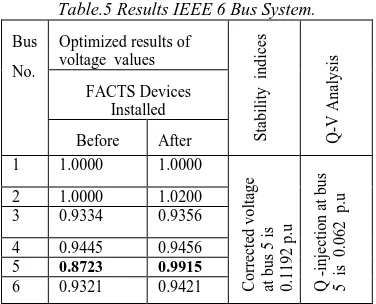
Table.5 Results IEEE 6 Bus System.
Bus
No.
Optimized results of voltage values
S ta b il it y in d ic es Q -V A n al y si s FACTS Devices Installed
Before After
1 1.0000 1.0000
C o rr ec ted v o lt ag e at b u s 5 is 0 .1 1 9 2 p .u Q -in je cti o n a t b u s 5 is 0 .0 6 2 p .u
2 1.0000 1.0200
3 0.9334 0.9356
4 0.9445 0.9456
5 0.8723 0.9915
6 0.9321 0.9421
To demonstrate the effectiveness of the proposed
RBFAtechnique, the 25 different optimization are
been carried out and the best solution of Tap setting
parameters are listed in Table.4.
5.3 IEEE6 Bus System
The extension of effective analysis of proposed technique analyzed with IEEE 6 bus system. The results of FLFI and VSA approaches and also optimized values are listed in Table.5. The results
of proposed technique, the critical line is 2-5 and weakest bus is bus number.5. Therefore the FACTS devices are installed in bus 5 and line 2 to 5, the corrected voltage and Q injection are tabulated in same table.
Table.6 Results IEEE 6 Bus System.
Bus
No.
Optimized results of voltage values
S ta b il it y in d ic es Q -V A n al y si s FACTS Devices Installed
Before After
1 1.0000 1.0000
C o rr ec ted v o lt ag e at b u s 5 is 0 .1 1 9 2 p .u Q -in je cti o n a t b u s 5 is 0 .0 6 2 p .u
2 1.0000 1.0200
3 0.9334 0.9356
4 0.9445 0.9456
5 0.8723 0.9915
6 0.9321 0.9421
5.4 IEEE9 Bus System
[image:13.612.101.289.438.590.2]The results of IEEE 9 bus system is listed in Table.6. In this case, the identification of weak bus is critical and because of real and reactive loading. The bus number 8 is most critical bus in IEEE9 bus system. Thus the results of FLFI and VSA approaches and the reactive power injection level is analyzed via Q-V analysis and Q-injection is listed in Table.6.
Table.7 Results IEEE 6 Bus System
Bus
No.
Optimized results of voltage values S ta b ility in d ices Q -V A n aly sis
FACTS Devices Installed
Before After
1 1.0400 1.0400
C or re ct ed vol ta ge a t bus 8 0. 076 5 p. u Q -in je ctio n a t b u s 8 is 0. 200 0 p. u
2 1.0162 1.0210
3 1.0134 1.0146
4 0.9925 1.0042
5 0.9523 0.9772
6 0.9645 0.9821
7 1.0040 1.0056
8 0.8656 0.9421
9 1.0057 1.0082
5.5 IEEE39 Bus System
[image:13.612.302.529.483.677.2]is not analyzed here but proposed approaches are listed in Table.7. The result of FLFI and VSA approaches are the weak bus identification is bus number 15. The reactive power injection and installation of FACTS devices are carried out by Q-V analysis. The Q-Values of index value and injection are listed in same Table.7.
5.6. Experimental Setup and Function Optimization
In this section mainly focused about function optimization and how the validity analysis carried out. The different algorithms are taken for validity analysis and listed in above section. In all the experiments, the basic BFA, MBFA and proposed algorithm are considered same bacteria size and maximum numbers of generations are varied according to the function and trapping level of local minima. The initial solution is generated randomly according to the function and is given in [22].
Fig.6 Voltage Profile Optimization Of IEEE 30 Bus
Table.7 Results IEEE 39 Bus System
Most critical bus and corrected voltage drop
level
Q-V analysis
15 0.0721 Q -injection at bus 15 is
0.221 p.u with index value is 0.8714
5.7 Comparison of Results with Similar Bio-Inspired Algorithms
In order to strengthen the local search ability and to ability to track or attain the global optimal quickly, the bio-inspired algorithms are well suitable. The performance of proposed algorithm is compared with other bio- inspired algorithms like Ant Colony Algorithm (ACO), basic Bacterial Foraging Algorithm (BFA) and Modified version of Bacterial Foraging Algorithm (MBFA). All the above mentioned algorithms and proposed
algorithms are executed the same runs. The case studies and the results show the proposed algorithm is efficient in all categories. The application of proposed RBFA algorithm, the total real power losses is minimized during full load operating condition and during the optimization process the real power losses minimized with secured manner and all operating constraints are within the limits and this because of FLFI, VSA and Q-V analysis.
6. CONCLUSION
In this work, OPD is treated as a multiobjective problem and multidisciplinary problem by considering the multiple objectives of voltage profile, power loss, voltage deviation and optimal location of FACTS devices with reliability analysis of FLFI, VSA approaches and Q-V analysis. The validity analysis of proposed work has been carried out with help of IEEE 6, IEEE 9, IEEE 30 and New England IEEE 39 bus systems and the performance of proposed work is compared with various social foraging algorithms. The results of proposed work are well in speed of convergence, tracking of global solution and handling of control variables. The results are really encouraging and challengeable in multiobjective problems in deregulated power systems especially OPD problem.
REFERENCES
[1]. Kevin passion M, “Biomimicry of Bacterial
Foraging for distributed optimization and control,” IEEE Control Systems Magazine, 2002, vol.22: pp.52-67.
[2]. S.Jaganathan, S.Palaniswami, “New Refined
Bacterial Foraging Algorithm for Multi- Disciplinary and Multi-Objective Problems,” Journal of Computational Intelligence in Bioinformatics, Volume 5, Number 2 (2012) pp. 113-131.
[3]. A. Kazemi and B. Badrzadeh, “Modeling and
Simulation of SVC and TCSC to Study Their Limits on Maximum Loadability Point”, 2004, vol. 26, no. 5, pp.381-388.
[4]. A. Armbruster,M. Gosnell, B. McMillin, and
M.L. Crow, “The maximum flow algorithm applied to the placement and distributed steady-state control of UPFCs,” in Proceedings of the 37th Annual North American Power Symposium, 2005, pp. 77– 83.
[5]. S. Jaganathan, Dr.S. Palaniswami, G.
in Reactive power planning problem using a Ant colony Algorithm,” European Journal of Scientific Research, Issue 51, 2011, Vol 2,2011. ISSN 1450-216X Vol.51 No.2 ,241-253.
[6]. S.Jaganathan, Dr.S.Palaniswami, K.
Senthilkumaravel, and B. Rajesh, “Application of Multi- Objective Technique To Incorporate UPFC In Optimal Power Flow Using Modified Bacterial Foraging
Technique”, International Journal of
Computer Applications (0975 – 8887), 2011, Vol.51 No.2 ,241-253
[7]. S. Jaganathan, Dr. S. Palaniswami, C.
Sasikumar, ”Multi Objective Optimization for Transmission Network Expansion Planning using Modified Bacterial Foraging
Technique”, International Journal of
Computer Applications, 2010, (0975 – 8887).
[8]. L. Gyugyi, “A unified power flow control
concept for flexible AC transmission systems”, IEE Proc., Part-C, Vol.139, No.4, 1990, pp. 323-331.
[9]. S. Tarakalyani, G. Tulsiram das, “Simulation
of real and reactive power flow control with UPFC connected to a transmission line” Journal of Theoretical and Applied Information Technology,2008.
[10].J. Baskaran, V. Palanisamy, “Optimal
location of FACTS device in a power system network considering power loss using genetic algorithm” EE-Pub on line journal, 2005.
[11].R.T. Byerly, D.T. Poznaniak, E.R. Taylor,
“Static Reactive Compensation for Power Transmission System”,IEEE Trans. PAS-101, 1982, pp. 3998–4005.
[12].A.E. Hammad, “Analysis of Power System
Stability Enhancement by Static VAR Compensators”, IEEE Trans.PWRS, 1986, pp. 222–227.
[13].K.R Padiyar, R.K. Varma, “Damping Torque
Analysis of Static VAR System Oscillations”, IEEE Trans. PWRS, 1991, 6(2), pp. 458–465.
[14].E.Z Zhou, “Application of Static VAR
Compensators to Increase Power System Damping”, IEEE Trans. PWRS, 1993, pp. 655–661.
[15].Jose A. D. N, Jose L. N. A, Alexis D, Durlym
R and Emilio P.V, “Optimal parameters of FACTS devices in eclectic power systems applying evolutionary strategies,” Electrical Power and Energy Syst., vol. 29, pp.83-90, 2007.
[16].M.Basu, “Optimal power flow with FACTS
devices using differential evolution,”
Electrical Power and Energy Syst., vol.30. pp.150-156, 2008.
[17].S.Jaganathan, S.Palaniswami, “Solution Of
Multi – Objective Optimization Power System Problems Using Hybrid Algorithm,” Journal of Asian Scientific Research Applications, vol. 1 n.5, pp.26 5-270, 2011,.
[18].K Y Lee, Y M Park and J L Ortiz, 1985,”A
United Approach to Optimal Real and Reactive Power Dispatch”, IEEE Trans. On Power Systems vol14.no.5.
[19].Sheng-Huei Lee., Chia-Chi Chu, "Power
Flow Models of Unified Power Flow Controllers in Various Operating Modes" IEEE Trans. Power Elect, 2003, 0-7803-8110-6/03.
[20].Kundur P., 1994, Power System Stability and
Control, McGraw-Hills, Inc, New York.
[21].Allen J. Wood, Bruce F.Woolenberg.“ Power
system control and operation”, John Wiley & sons.
[22].S.Jaganathan,S.Palaniswami, “Application of
Multi-objective Optimization for Optimal Parameters of IPFC and Optimal Power Flow (OPF) with IPFC using FBFA,”IEEE tencon2011, Indonesia , pp.445-449,Balli, November 2011.
[23].ZHAO Bo, CAO Yi-jia, “Multiple objective