184
BIOMEDICAL SIGNALS ANALYSIS BY DWT SIGNAL
DENOISING WITH NEURAL NETWORKS
GEETA KAUSHIK1, DR. H.P.SINHA2, DR. LILLIE DEWAN3
Associate Professor,Maharishi Markandeshwar Engineering College, Electronics and Communication, Maharishi Markandeshwar University,
#380-81, New Vashisht Nagar, Ambala Cantt1 Associate Director & Head Ece Deptt.,
Mmu, Mullana Ambala2 Professor, Nit, Kurukshetra3
E-mail: [email protected], [email protected],[email protected]
ABSTRACT
The core intention of this work is to investigate the wavelet function that is optimum in identifying and denoising the various biomedical signals. Using traditional methods it is difficult to recover the noises present in the signals. This paper presents a detail analysis of Discrete Wavelet Transform (DWT) denoising on various wavelet families and biomedical signals such as ECG, EMG and EEG. We have developed a trained network in order to optimally denoise the signals by using a back propagation algorithm in the neural network. Initially noise is added to the original signal, then the signal is decomposed using the Shift Invariant method. After decomposition, the proposed wavelet based method is used for noise removal. Then the signal is reconstructed by using wavelet reconstruction method. The denoised signals will be compressed by a hybrid wavelet shannon fano coding for reducing its storage size. Keywords:- DWT, ECG, EEG, EMG, Neural network, Wavelet frequency thresholding
1. INTRODUCTION
A signal is a physical quantity which differs with respect to time, space and contains information from the source to the destination. The signal processing indicates any manual or mechanical operation which modifies, analyzes or else manipulates the information contained in a signal [1]. In the application of signal processing, wavelets provide a mathematical tool for the hierarchical decomposition of functions in signal and image processing [2]. The noise is the most important problem in signal processing. Noise removal can be done by removal of small coefficients. The noise consists of high frequency components that are referred as linear denoising.
The corresponding scales of the Wavelet Transform are set to zero. Noise assumed by non-linear denoising or wavelet shrinkage consists of low energy [3].
Signal denoising refers to the process of removing the noise from a signal. It is the main problem in
signal processing. To estimate a clean version of a given noisy signal is the main goal of natural signal denoising [4]. The noise may corrupt the signal in many cases in a significant manner and it must be removed from the data in order to proceed with further data analysis. While denoising the signal it will improve perceptual quality, compression effectiveness and the accuracy of signals [5]. Using simple filtering operations it is very difficult to remove the noises [6] and by using the traditional methods it is difficult to recover the noises present in the signals.
When we try to achieve good performance of EEG signals, the major problem that occurs here is the noisy EMG signals [12]. The biomedical signals may easily affected by noise and detecting these noises in the signals by using powerful and advance methodologies is becoming a very important requirement.
In general, a wavelet is a wave like oscillation with the amplitude starting at zero, increasing and then decreasing to zero. The main function of wavelet transform is used to reduce the unwanted noise and blurring in the signals [8]. Wavelet transform is the best technique used for denoising the signals [7]. Wavelet transform achieves a correlation analysis; consequently the output is expected to be maximal when the input signal mostly resembles the mother wavelet. The wavelet denoising methods offer high quality and flexibility for the noise problem of signals and images. The Discrete Wavelet Transform (DWT) is based on performance in order to meet the mathematical criteria to obtain the discrete sequences as discrete wavelet functions. If the analyzing function is waveform adapted, then DWT based denoising can be performed better [9]. Dividing the continuous time function into wavelets is referred to us Continuous Wavelet Transform (CWT).
In general, the term signal decomposition is referred to as the way of decomposing a given signal into a sum of simpler signals. To have a scale invariant interpretation of the image enables multi-resolution decomposition [4]. Decomposing a signal into scales with different time and frequency resolutions is done by a Multi-Resolution Analysis (MRA) algorithm [13]. The small number of resulting coefficients is relatively good decomposition. To decompose a signal, wavelet transform uses some set of basic functions [9]. By means of classification of spectral peaks, transient spectral peaks were detected and were investigated into distinction the between sinusoidal and noise components. The classification is based on descriptors derived from properties related to time-frequency distributions [15].
There are many types of wavelets. The Daubechies wavelet is described by a maximal number of vanishing moments for some given support and the Haar wavelet is an order of rescaled square shaped function which together forms a wavelet family. Symlet wavelets are only an improved version of Daubechies wavelets with an increased symmetry while the Coiflet wavelets have scaling functions
with vanishing moments. The Mathieu equation is a second order differential equation with periodic coefficients and the Legendre function has common applications in which spherical coordinate system are suitable.
Signal reconstruction generally means that the determination is of an original continuous signal from an order of equally spaced samples. Reconstructing the original sequence from the thresholded wavelet detail coefficients leads to a denoised (smoothed) version of the original sequence. Inverse Discrete Wavelet Transform (IDWT) is used to reconstruct the original signal. Calculate high resolution log-spectral features of the input noise signal to reconstruct the signal [17]. Therefore, wavelet transform is a reliable and a much better technique than the Fourier transform technique. Biomedical signals require high storage to be stored and high bandwidth to be transmitted. Compression of the signals refers to reducing the redundancy in it. Signal compression techniques are limited to the amount of time required for compression and reconstruction, the noise embedded in the raw signal and the need for accurate reconstruction of the waves [18].
2. RELATED WORKS
Hari Mohan Rai et.al [6] utilized Haar, Daubechies and Symlets wavelet families for De-noising. For removing the noise from the ECG signals they used three different wavelet families (Haar, Daubechies and Symlets). The different noise structure (unscaled white noise, scaled white noise and non white noise) had been selected for ECG signals and then compared their statistical parameter to find out the best result.
Zoltan German-Sallo et.al [9] proposed the design of the waveform-adapted analyzing function to have a good wavelet decomposition of the analyzed signal. A good decomposition means a relatively small number of resulting coefficients and a good reconstruction of the signal from these. Their proposed procedure led to obtain discrete sequences as discrete wavelet functions to perform denoising, these met certain mathematical criteria. Discrete Wavelet Transform based denoising was performed. A waveform-adapted wavelet transform based noise suppression procedure was introduced and the experimental result was obtained.
186 shift variance in the discrete wavelet transform (DWT). He has described a generalization of the critically sampled DWT and the fully sampled algorithm that provides approximate shift-invariance with an acceptable level of redundancy. They had proposed over complete DWT (OCDWT) is critically sub-sampled to a given level of the decomposition below which it is then fully sampled. This proposed algorithm illustrated in an edge detection context and directly compared to a number of other shift-invariant transforms in terms of complexity and redundancy.
Yousef M. Hawwar et.al [21] presented the effectiveness of both soft and hard thresholding for desired detail levels. Filtering noise in real time has applications in speech and image processing. Considerable interest has arisen in recent years regarding filtering in the wavelet transform domain. This technique has been effective in noise removal with minimum side effects on important features such as image details and edges. An efficient hardware implementation based on the FPGA technology was proposed.
G. Umamaheswara Reddy et.al [23] introduced a new wavelet threshold method namely wavelet threshold method with Grey Incidence Degree (GID) (or the GID threshold method). It showed that the signal smoothness and similarity of the two signal criteria have been greatly improved by the GID threshold method compared with existing threshold methods. According to the characteristics of different ECG signals, the GID threshold method gets better results than it can adaptively deal with noise separation and details remaining of the two opposing signal problems so as to provide a better choice for wavelet threshold methods of signal processing. Performance analysis was performed by evaluating the Mean Square Error (MSE), Signal-to-noise ratio (SNR) and visual inspection over the denoised signal from each algorithm. Their experimental result shows that the GID hard shrinkage method with sub-band or level dependent thresholding gives the best denoising performance on an ECG signal. The result shows that soft threshold will not always give better denoising performance; it depended on which wavelet thresholding algorithm was chosen.
Moshe Mishali et.al [20] described how to choose the parameters of the multi-coset sampling so that a unique multiband signal matches the given samples. To recover the signal the continuous reconstruction is replaced by a single finite-dimensional problem
without the need for discretization. The resulting problem was studied within the framework of compressed sensing, thus it can be solved efficiently using known tractable algorithms from this emerging area. They also developed a theoretical lower bound on the average sampling rate required for blind signal reconstruction which is twice the minimal rate of known-spectrum recovery. They had ensured a perfect reconstruction for a wide class of signals sampled at the minimal rate and provides a first systematic study of compressed sensing in a truly analog setting. Various experiments are presented by demonstrating blind sampling and reconstruction with minimal sampling rate.
Omerhodzic et.al [11] had implemented a wavelet-based neural network (WNN) classifier for recognizing EEG signals and tested it under three sets of EEG signals (healthy subjects, patients with epilepsy and patients with epileptic syndrome during the seizure). First, the Discrete Wavelet Transform (DWT) with the Multi-Resolution Analysis (MRA) was applied to decompose an EEG signal at resolution levels of the components of the EEG signal (δ, θ, α, β and γ) and the Parseval’s theorem was employed to extract the percentage distribution of energy features of the EEG signal at different resolution levels. Second, the neural network (NN) classifies these extracted features to identify the EEG’s type according to the percentage distribution of energy features. The performance of the proposed algorithm had been evaluated using a total of 300 EEG signals. The results showed that the proposed classifier has the ability of recognizing and classifying the EEG signals efficiently.
3. MAIN CONTRIBUTIONS
Signal denoising is to estimate a clean version of a given noisy signal. In the existing system, while denoising the biomedical signals such as ECG, EEG and EMG, the trained system is unable to automatically detect the best wavelet suitable for denoising. The Fourier transform analysis is inadequate and is localized only in the frequency band. The major drawback of Short Term Fourier Transform for signal denoising is that the time frequency precision is not optimal. Digital filters and adaptive methods can be applied only to signals whose statistical characteristics are stationary in many cases and cannot be applied to non-stationary signals because of loss of information.
To overcome these drawbacks wavelet transform is introduced and Discrete Wavelet Transform is used for denoising. Our proposed method can be applied to both stationary and non-stationary signals. The wavelet transform analyzes the signal both in time and frequency domains. In this proposed method a trained system automatically classifies which wavelet is best suitable for denoising the three kinds of biomedical signals such as ECG, EEG and EMG signals. Thus Wavelet transform will be the better choice while comparing it to the other techniques.
In this paper, the DWT based denoising was accomplished in eliminating the noise from the three types of signals. Wavelet functions and Grey incidence thresholding rules were considered to evaluate the efficiency on noise removal from the signals. After that, classify the wavelet which is best suited for denoising using a neural network classifier.The organization of this paper is given as follows: section 4 describes the proposed methodology of DWT based denoising of biomedical signals using the thresholding method, section 5 describes the mathematical model and finally the conclusion is given in section 9.
4. PROPOSED METHODOLOGY
The original signal is assumed as o(n) and the white Gaussian noise is assumed as e(n). By accumulating these signals the noisy signal s(n) will be attained. It is typically of the form
s(n) = o(n) + e(n)
(1)
The general wavelet based denoising procedures are composed of these steps:
Decomposition: A wavelet function is chosen and decomposed upto level l.
Denoising wavelet detail coefficients: For every level of decomposition, select a threshold value and apply thresholding to the detail coefficients.
Reconstruction: Calculate the reconstruction based on the approximation coefficients of level l and the modified detail coefficients of levels from 1 to l.
Classifier: A Classifier achieves its objective by making a classification decision based on some characteristics.
Compression: Reducing the amount of bits essential to define a signal to an approved accuracy.
Wavelet transform is a mathematical tool for processing one-dimensional or multidimensional signals [24]. The scalar wavelet transform has been widely used in many applications like signal de-noising, image compression and in medical applications as well. In the preceding two decades wavelet transform based de-noising was the best alternative for Fourier transform based signal de-noising [25]. The first step of the De-de-noising procedure using wavelet transform is selection of
the mother wavelet –
ψ
m,n(
t
)
which forms a set of functions (family of wavelets), by compression or stretching or translation. The next step is the decomposition level. An example for a mother wavelet equation is as follows:(1) Where
n = coefficient of time translation, m = coefficient of scale (compression).
Noise reduction plays a major role in signal processing. The various noise structures in different biomedical signals are unscaled white noise, scaled white noise, non white noise, white Gaussian noise etc. Wavelet Thresholding, Wavelet Shrinkage and Non-linear Shrinkage are widely used terms for wavelet domain denoising. The wavelet which is similar to the signal is selected for signal denoising. The proposed technique is opted to implement using MATLAB 7.10 tool and will be evaluated
)
2
(
2
)
(
2,
t
t
n
m m
n
m
=
−
−
188 using the database signals such as MIT-BIH arrhythmias and Sleep-EDF databases.
4.1 Wavelet transform
An indispensable tool for a variety of applications such as classification, compression and estimation is wavelet transform. Signal information in wavelet development is conveyed by a comparatively small number of large coefficients. This property of the wavelet transform makes the use of wavelets mainly ideal in signal estimation. It has been revealed that wavelets can eliminate noise more effectively than previously used methods.
Wavelet transforms can decompose a signal into numerous scales that represent dissimilar frequency bands and at each scale, the position of the signal’s instantaneous structures can be determined approximately. The purpose is to satisfy certain mathematical necessities and is used in representing data or other functions of a wavelet. The Wavelet Transform provides a time-frequency illustration of the signal. The signals are examined and expressed as a linear combination of the sum of the product of the wavelet coefficients and a mother wavelet by wavelet transform [10]. The original signal is transformed using predefined wavelets in wavelet transform. The wavelets are orthogonal, biorthogonal and multiwavelets. By calculating signal to noise ratio of the signal the accuracy of the wavelet transform is determined after reconstruction of a signal. The wavelet transform is given by:
( )
x
t
dt
c
d
t
K
c
d
c
X
w,
1
∫
(
)
∞
∞ −
−
∗
=
( 2 )
where c and d are wavelet function parameters and x(t) is the signal to be transformed. Some of the applications identify pure frequencies, de-noising signals, compressing images, detecting discontinuities, breakdown points and self-similarity.
4.1.1 Discrete Wavelet Transform
Discrete wavelet transform is the same as filtering it by a bank of filters of non-overlapping bandwidths which vary by an octave. It is based on sub-band coding which is found to yield a fast calculation of Wavelet Transform. It is easy to implement and diminish the calculation time and resources required. A set of dilations and
translations
ψ
i,j(
t
)
of a preferred mother wavelet)
(t
ψ
is used for signal analysis. It is important toknow the behavior of these filters with these wavelet coefficients. According to the mother wavelet design the coefficients of these filter banks are determined. A common equation for the Discrete Wavelet Transform signal is written as:
[ ] [ ]
∑
∞−∞ =
=
mf
e
m
m
x
f
e
X
[
,
]
ϕ
,( 3 )
Where,
ϕ
[ ]
m
be the window of finite length, f is a real number known as window translation parameter and e is a positive real number named as contraction parameter.4.1.2 Continuous wavelet transform
The continuous wavelet transform (CWT) converts a continuous signal into extremely redundant signal of dual continuous variables: translation and scale. The resulting changed signal is easy to interpret and valuable for time-frequency analysis [26].
dt
d
c
t
t
g
d
d
c
g
∫
∞
∞ −
−
=
(
)
ϕ
)
,
(
12( 4 )
Where c, d ∈ R, c ≠ 0 and they are dilating and translating coefficients respectively.
4.2 Wavelet filters
Discrete Wavelet Transform is performed by repeated filtering of the input signal using two filters. The filters are a low pass filter (LPF) and a high pass filter (HPF) to decompose the signal into different scales. The output coefficient gained by the low pass filter is the approximation coefficient. The scaling function output is in the form of:
∑
=
−
=
Mq
q
t
q
h
t
0
)
2
(
)
(
2
)
(
ϕ
ϕ
( 5 )
The output of the high pass filter is the detailed coefficient. The wavelet function output is in the form of:
∑
=
−
=
Mq
q
t
q
g
t
w
0
)
2
(
)
(
2
)
(
ϕ
( 6 )
frequency response is achieved from the given input signal [16,18].
4.3 Wavelet families
Table 1.Wavelet families
Wavelength families are listed above in Table 1 with respect to wavelets.
4.3.1 Daubachies
Commonly Daubechies family wavelets are signed dbN (N is the order). This wavelet belongs to the orthogonal wavelets.
4.3.2 Coiflets
A discrete wavelet was designed by Ingrid Daubechies to have a scaling function with vanishing moments. The scaling function and the wavelet function must be normalized by a common factor. By retrogressive the order of the scaling task coefficients and then reversing the symbol of every second one is the wavelet coefficients.
4.3.3 Symlets
The symlet family wavelets are signed symN (N is the order). The symlets are nearly symmetrical, orthogonal and biorthogonal wavelets suggested by Daubechies as modifications to the db family. The properties of the two wavelet families are similar [19].
4.3.4 Biorthogonal
Biorthogonal filters state a superset of orthogonal wavelet filters and have found their use virtually in all areas where wavelets are used. The biorthogonal family wavelets are signed as bior. Biorthogonal wavelet transform has frequently been used in numerous image processing applications, because it makes multi-resolution analysis possible and does not produce redundant information.
4.4 Wavelet decomposition
In Wavelet decomposition, it is possible to alter the resulting coefficient previously for a signal and signal reconstruction is to eliminate undesirable
signal components. Choose a wavelet function with level N. Calculate the wavelet decomposition of the signals at level N [6].
4.4.1 Shift invariant method
The commonly referred algorithm trous, which is to make the DWT shift-invariant is not to do any subsampling at all. The à trous algorithm is
shift-invariant and it can be used with some of the mother wavelets usually used with the DWT [22]. Only the mother wavelet has to be expanded, there is no sub-sampling of data performed at each level of the transform.
4.4.2 Empirical Mode Decomposition
Emprical Mode Decomposition is especially related for nonlinear and non-stationary signals. The calculation of EMD does not require any previously known value of the signal [10]. Emprical mode decomposition adaptively decomposes a multicomponent signal into intrinsic mode functions (IMF). The fact that the functions into which a signal is decomposed are all in the time domain and of the same length as the original signal permits for variable frequency in time to be conserved. By gaining IMF from real world signals it is essential because natural processes often have multiple causes. And every cause may happen at specific time intervals. In EMD analysis this kind of data is evident, but quite secreted in the Fourier domain.
This technique is faced with the difficulty of being fundamentally defined by an algorithm, and therefore of not acknowledging an analytical formulation which would permit a theoretical investigation and performance estimation. Some initial elements of investigational performance evaluation will also be provided for giving an essence of the efficiency of the decomposition as well as of the trouble of its interpretation.
4.4.3 Multi-resolution analysis
In any discrete wavelet transform there are only a limited number of wavelet coefficients for each bounded rectangular region in the upper halfplane. Each coefficient needs the evaluation of an integral. A multiresolution representation presents an uncomplicated hierarchical framework for interpretating the image information. This method is performed on the wavelet coefficients directly.
4.5 Wavelet thresholding
Choice of a suitable wavelet function, thresholding methods and the thresholding rule play a vital role in signal denoising [16]. Thresholding methods used with discrete wavelet transform based filtering are to modify the obtained coefficients. By using Wavelet
Families
Wavelets
Daubechies 'db1' or 'haar', 'db2', ... ,'db10', ... , 'db45' Coiflets 'coif1', ... , 'coif5'
Symlets 'sym2', ... , 'sym8', ... ,'sym45' Discrete
Meyer
'dmey'
Biorthogonal 'bior1.1', 'bior1.3', 'bior1.5'
190 wavelet thresholding the noise in the signals can be removed. There are several methods to choose the best analyzing function, the type of thresholding and the threshold values [9]. Threshold which is proportional to the standard deviation of the noise is the universal threshold T, and is defined as:
InM
T
=
σ
2
( 7 )Where, M represents signal size and
σ
2represents the noise variance, and it is given by( )
(
)
=
6745
.
0
2
median
X
iσ
( 8 )Where, (|Xi|) represents the median value of the
absolute values of wavelet coefficients Xi. Hard
thresholding:
( )
[
]
( )
[
]
≤
≥
=
0.55 . 0
ln
414
.
1
,
0
ln
414
.
1
,
L
x
L
x
x
x
i i i iσ
σ
( 9 )
Where,
1
.
414
σ
[
ln
( )
L
]
0.5 is the threshold value.Soft thresholding
( )
[
]
(
)
[
( )
]
( )
[
]
≤
≥
−
=
5 . 0 5 . 0 5 . 0ln
414
.
1
,
0
ln
414
.
1
,
ln
414
.
1
L
x
L
x
L
x
x
x
x
i i i i i iσ
σ
σ
( 10 )
4.5.1 Wavelet frequency thresholding
The basic idea of wavelet frequency thresholding is based on judging the extent of their relation from the similarity to orders of geometric curve shapes. The closer those are, the greater frequency thresholding of the corresponding order is and vice versa. According to this, we can compute the wavelet frequency analysis of the wavelet coefficients according to the relationship among the approximate time sequences. This method not only can filter most of the noise, but it can commendably also hold signal details. More than that, this technique can commendably compromise the problem of signal details remaining and noise suppression as well. For this reason the signal processed by wavelet frequency thresholding has a better smoothness and similarity [23]. Generally
wavelet frequency thresholding is represented by the given equation:
∑
==
m l it
m
1)
(
1
δ
δ
( 11 )4.5.2 EMD-Thresholding
EMD achieves a sub band like filtering resulting in fundamentally uncorrelated IMFs. Although the corresponding filter-bank arrangement is by no means pre-determined and fixed as in wavelet decomposition, one can accomplish thresholding in each IMF in order to nearly ignore low energy IMF parts which are expected to be significantly despoiled by noise [14]. The Empirical mode decomposition is an adaptive data-driven technique which is used for effective decomposition of a noisy signal into its functional components.
4.5.3 Wavelet based thresholding
Wavelet based nonlinear thresholding is effective for noise reduction only to the extent to which the wavelet representation of the noise-free signal is sparse. An efficient method of noise reduction only to the extent to which the wavelet representation of the noise free signal is sparse is wavelet based thresholding [8]. In this method the process of each coefficient from the detail sub bands with thresholding function is applied to obtain the output.
4.6 Wavelet reconstruction
The original signal is produced from the wavelet coefficients in most of the wavelet transform applications. The analysis and synthesis filters have to fulfill certain criteria to achieve a perfect reconstruction. Using the wavelet coefficients the original signal was reconstructed by applying inverse wavelet transform. The procedure of wavelet reconstruction comprises of up sampling by inserting zeros among the samples and filtering to expansion of the signal. A global reconstruction of the denoised signal is given by
∑
∑
= = ≈ ∧ ++
=
21 21
)
(
)
(
)
(
( ) ) ( N N j P N j j jt
K
t
K
t
y
( 12 )
4.7 Neural Network classifier
on to the following layer. Normally the networks are defined to be feed-forward in which a unit feeds its output to all the units on the following layer, but there is no feedback to the previous layer. Feed-forward ANNs allow signals to travel one way only; from input to output. There is no feedback (loops) i.e. the output of any layer does not affect that same layer. Feed-forward ANNs tend to be frank networks that associate inputs with outputs. They are sketchily used in pattern recognition. This category of group is also referred to as bottom-up or top-down. In fig1. Neural network classifier Debited
Fig1. Neural Network
Weightings are applied to the signals transient from one unit to another and it is these weightings which are adjusted in the training phase to adapt a neural network to the particular problem at hand, this is the learning phase. These range from role illustrations to pattern recognitions, which is what we will consider.
For example, consider a finite sequence of input signals as X = (X1,X2,……,Xn), the signal Pn where
n = 1,2,…..N, may be real numbers or vectors. By introducing a transfer function that depends on a certain parameter vector H = (H1,H2,……,Hm).
Consequently, Y will be elected according to a chosen optimality criterion. The optimization is typically carried out in such a way that the sequence of model output signals Y = (Y1,Y2,…,
Yn) generated by the function f = f(H,P) is as close
as possible to the corresponding set of observations P = (P1,P2,…,Pn).
Feedback networks are used to implement optimization problems. Feedback paths with these networks are interconnected with the neurons. Neurons express the differential equation given as:
j i m
i ji j
j j
J
x
R
u
dt
du
+
+
−
=
∑
=1
φ
( 13 )
Where,
x
i=
h
(
u
i)
, i=1,2,…m and h( ) is the sigmoid activation function.4.7.1 Back Propagation Neural Network
Backpropagation neural network is the occurrence in which the action potential of a neuron produces a voltage spike mutually at the end of the axon (normal propagation) and back through to the dendritic arbor or dendrites, from which of the original input current initiated. It has been revealed that this uncomplicated process can be used in a manner similar to the backpropagation algorithm used in multilayer perceptrons, a type of artificial neural network. An action potential extends down the axon because of the gating properties of voltage-gated sodium channels and voltage-gated potassium channels.
4.8 Signal compression
Signal compression is essential because the sum of data that has to be transmitted may exceeds the carrying volume of most networks. Data rate is measured in bits per second and the data rate is determined by the volume of the carrier medium which is also measured in bps. In discrete wavelet transform the most prominent information in the signal emerges in high amplitudes and not much of prominent information emerges in very low amplitudes. Data compression can be achieved by removing these smaller amplitudes. High compression ratio with good quality of reconstruction is achieved by wavelet transform. By using wavelet transform high compression ratio with excellent reconstruction is achieved. The long-lasting proliferation of computerized biomedical signal processing systems along with the increased characteristic performance requirements and demand for lesser cost medical care have mandated reliable, accurate, more efficient biomedical data compression techniques [27].
4.8.2 EBP-ANN Based Data Compression Initially the network is trained for the signal to be compressed. After successful training the trained weights between the output and hidden layer and the activation levels of the hidden layer units are stored during compression. The stored information needs less space and is used for reconstruction of the original signal.
4.8.3 QRS-complex detection and estimation
192 complex as well as spikes from high-frequency pacemakers can cooperate with the detection of the QRS complex as shown in fig2. In addition there are numerous sources of noise in a clinical atmosphere that can damage the ECG signal[34].
Fig2.Important features of ECG signal
4.8.4 Shannon-fano algorithm
Every signal has a dissimilar number of bits. According to probability these are arranged in descending order. The lower occurrence probability is stored by a larger number of bits and the higher occurrence probability is stored by a lesser number of bits. For the decompression algorithm, the signals of different length are not a barrier.
5. MATHEMATICAL MODEL
The original signal is assumed as o(n) and the white gaussian noise is assumed as e(n). By accumulating these signals the noisy signal s(n) can be attained. It is typically of the form
s(n) = o(n) + e(n)
The discrete wavelet transform is given as a function f(x) which can be represented by the super
position of daughters
ψ
c,d(
t
)
of a mother wavelet)
(t
ψ
whereψ
c,d(
t
)
can be expressed by
−
=
d
c
t
c
t
d cψ
ψ
,(
)
1
Discrete Wavelet Transform is performed by repeated filtering of the input signal using two filters. The filters are a low pass filter (LPF) and a high pass filter (HPF) to decompose the signal into different scales. The output coefficient gained by the low pass filter is the approximation coefficient. This is expressed as:
[ ]
[ ]
−
∗
<
∗
=
+otherwise
n
N
k
a
N
i
n
k
a
n
a
i i i i,
,
2
]
[
1The output coefficient of the high pass filter is detailed coefficient. This is expressed as
[ ]
[ ]
[ ]
−
∗
<
∗
=
+otherwise
n
N
f
a
N
i
n
f
a
n
y
i i i i,
,
2
1The approximation coefficient is then divided into
detail and approximation coefficients. This is
expressed as given below:
[ ]
[ ]
[ ]
[ ]
[ ]
(
)
∗ + ∗ < ∗ + ∗ = − + − + + + otherwise n f y n k a N i n f y n k a n a N i i N i i j i i , ˆ ˆ 2 / 1 , 2 ˆ ˆ 1 1 1 1 ( (And the process is repeated to N levels.
The next step is to calculate the noise intensity for
various levels,
( )
=
6745
.
0
j jd
median
α
)
(
2
In
L
and
η
j=
α
The output of the wavelet decomposition is the approximation and the detail coefficients are obtained in every level of decomposition. Then calculate the wavelet frequency thresholding between the detail coefficient and the approximation coefficient by the following steps:
1. Calculate the mappings of the initial values for various sequences. Let
)
1
(
' j jj
Y
y
Y
=
where j=0,1,… ..,M.
2. Calculate the difference of the mappings.
Let
Ω
j=
(
Ω
j(
1
),
Ω
j(
2
),...,
Ω
j(
n
)
)
WhereΩ
j(
g
)
=
x
0'(
g
)
−
x
'j(
g
)
and j=0,1,2,……,N.3. Calculate the biggest and smallest
difference of
Ω
j(g
)
. Let R=)
(
max
max
jg
g
j
Ω
and
r=
min
min
j(
g
)
g jΩ
))
(
),...,
2
(
),
1
(
(
y
'jy
'jy
'jn
4. Calculate the incident co-efficients
R
g
R
r
g
j
j
ϑ
ϑ
γ
+
Ω
+
=
)
(
)
(
Where
ϑ
∈
( )
0
,
1
;y=1,2,…………..,n and j=0,1,2,…..,N5. Calculate the wavelet frequency
thresholding. So
∑
=
=
ng
j
g
n
1)
(
1
γ
γ
where j=0,1,2,…….N .
(
)
)
(
max
max
)
(
)
(
)
(
)
(
max
max
)
(
)
(
min
min
)
(
),
(
)
(
0 0
g
x
x
g
x
g
x
g
x
g
x
g
x
g
x
g
x
g
x
g
j o g j j
o
j g
i j
o g j j oj
−
+
−
−
+
−
=
=
ϑ
ϑ
γ
γ
According to the mentioned method calculate the
threshold
η
THR=
η
j•
γ
j then maintain the original value when a position wavelet transform coefficient value is larger than the threshold, otherwise let the value be zero.6. Calculate the threshold by using the
formula
[ ]
24
n
S
THR
=
, where S[n] is theoriginal signal.
After that the reconstruction can be done to produce
the original signal. This is an inverse process of
decomposition and the denoised signal will be
obtained. In order to find the optimized wavelet the
signal is trained in the neural network with the
features present in the signal. The inputs are labeled
as x1,x2,…..,xm and the weights are labeled as
w1,w2,….,wm. The weighted sum of input values are
represented as
∑
=
=
mj j j
x
w
1ω
After that, the signals are compressed through the
probabilities of the source produce symbols. The
probabilities are q1,q2,……,qn, and the entropy is
given by:
∑
=
−
=
mj
j
j
q
q
V
0
2
log
After the compression has been successfully
completed the signals are stored in a database.
5.1 FLOW CHART
In fig.3 shows flow chart about optimized wavelet.
Fig3.Flowchart
6. PROPOSED BLOCK DIAGRAM
Neurons
Fig4.Neural Network Denoising and Compression
In fig4.shows signal denoising and compression. The signal is decomposed and then reconstructed upto level 3. For example, consider the signal is denoted as Sj+1. In the synthesis filter the signal is
then decomposed using a high pass filter which is denoted as Ho(n) and a low pass filter which is
denoted as Hl(n) and as a result the detail Signal
Denoising
Signal compression
Neural network
Optimized wavelet
Wavelet Frequency Thresholdi ng
Denoi sed Signal Input
Sign al
194 coefficient dj and approximation coefficient aj are
gained. Then in the next level of decomposition the approximation coefficients are again decomposed and the process is repeated upto N levels.
By using the coefficients gained at every level calculate the threshold value by using the wavelet frequency thresholding method. After the calculation of the threshold value, the coefficients above the threshold value remain constant and the coefficients which are below the threshold value are changed as zero.
In the reconstruction stage the coefficients are fed as an input to the analysis filter. Here the reverse process of decomposition will be done and the output will be the denoised signal Sj+1.
The signals are compressed using compression techniques. The signals are then fed as the input, when the compressions have been over the compressed signal will be attained as the output and these signals are stored in a database as per shown in Fig5.
Fig5.Signal compression
The input of the neural network will be the samples from numerous channels which is equivalent to the time segments with a constant length. The target channel equivalent to the time segment used in the input will be the output [28]. The preprocessed signals will be trained in the neural network to automatically predict which wavelet is best suitable for denoising and compression.
7. METHODS
The biomedical signals are collected from the databases and the databases enclose the signals without noise. Subsequently the noise is added to those signals by using a MATLAB program and then the number of samples is chosen for further processing. In this experiment 40,000 samples of the signals are chosen and calculated are a variety of statistical parameters of the noisy biomedical signals. The noisy signals are decomposed at level three using various wavelet families. De-noising of the signals has been performed based on the selected threshold value. By using the parameters
select the optimized wavelet transform which is best suitable for denoising using the neural network classifier and then these signals are compressed.
7.1 Signal to Noise Ratio
The signal to noise ratio is the ratio of the true signal amplitude to the standard deviation of the noise. The quality of the signal is termed as the signal-to-noise ratio, which is expressed as:
noise original
S
S
SNR
=
10
log
Where,
S
original represents the original signalwithout noise and
S
noise represents the noisy signal.7.2 Mean Square Error
The difference between the denoisied signal and the original signal is given by the following equation:
( ) ( )
(
)
21
1
∑
=
−
=
Mj
j
y
j
y
M
MSE
Where,
y
( )
j
represents the original signal,y
( )
j
represents the denoised signal and M represents the length of the signal.7.3 Compression Ratio
100 *
gnal Originalsi
al ressedsign Sizeofcomp inalsignal
Sizeoforig nRatio
Compressio = −
7.4 Compression Factor
n compressio ignalafter
Sizeofthes
on ecompressi ignalbefor
Sizeofthes nFactor
Compressio =
8. EXPERIMENTS AND RESULTS
We have experimented our proposed wavelet denoising method in various biomedical signals such as ECG, EEG and EMG signals taken from the MIT-BIH database. By using wavelet toolbox from MATLAB environment we have experimented our denoising approach. We have trained the neural network classifier to select the best suitable wavelet type for each kind of signal. In the training stage we have denoised the signals
Comp ressed signal Input
signal
Com press ion
Stored in Databa
by all wavelets and the best resulting wavelet is selected based on the results obtained. The conventional parameters such as PSNR and PRD are compared to find the optimal denoising wavelet. The tables 2,3,4,5,6 and 7show the denoising output of ECG, EEG and EMG signals respectively.
8.1 Training stage denoising results:
We have analyzed the denoising outputs and the optimal denoising wavelets for the three kinds of bio-medical signals. It also demonstrates the optimal denoising wavelets for ECG, EEG and EMG signals.
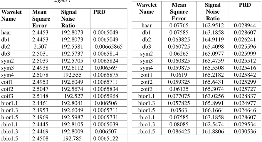
[image:12.612.88.534.302.543.2]ECG Signals
Table 2. Denoising results of different wavelets for ECG signal 1
Table3. Denoising results of different wavelets for ECG signal 2
Wavelet Name
Mean Square Error
Signal Noise Ratio
PRD
haar 2.5234 192.4924 0.0066082 db1 2.5234 192.4924 0.0066082 db2 2.5086 192.5514 0.0065887 db3 2.4922 192.617 0.0065671
sym2 2.5008 192.5826 0.0065784 sym3 2.4932 192.6108 0.0065692 sym4 2.5047 192.567 0.0065836 coif1 2.5063 192.5608 0.0065856 coif2 2.507 192.5577 0.0065866 coif3 2.5063 192.5608 0.0065856 bior1.1 2.5125 192.5359 0.0065938 bior1.3 2.5055 192.5639 0.0065846 bior1.5 2.5125 192.5359 0.0065938 rbio1.1 2.5133 192.5328 0.0065948 rbio1.3 2.5438 192.4123 0.0066347 rbio1.5 2.5297 192.4677 0.0066163
EEG Signals
Table4. Denoising results of different wavelets for EEG signal 1
Wavelet Name
Mean Square Error
Signal Noise Ratio
PRD
haar 2.4453 192.8073 0.0065049 db1 2.4453 192.8073 0.0065049 db2 2.507 192.5581 0.00665865 db3 2.5031 192.5737 0.0065814 sym2 2.5039 192.5705 0.0065824 sym3 2.4938 192.6112 0.006569 sym4 2.5078 192.555 0.0065875 coif1 2.4953 192.6049 0.0065711 coif2 2.5047 192.5674 0.0065834 coif3 2.5148 192.527 0.0065968 bior1.1 2.4461 192.8041 0.006506 bior1.3 2.4953 192.6049 0.0065711 bior1.5 2.4969 192.5987 0.0065731 rbio1.1 2.4445 192.8105 0.0065039 rbio1.3 2.4469 192.8009 0.006507 rbio1.5 2.4508 192.785 0.0065122
Wavelet Name
Mean Square
Error
Signal Noise Ratio
PRD
196 Table5. Denoising results of different wavelets for
EEG signal 2
EMG Signals
Table6. Denoising results of different wavelets for EMG signal 1
Table7. Denoising results of different wavelets for EMG signal 2
Compression Result
Table8. Compression Results of different wavelets for a sample signal
The comparison results for denoising are presented in the above Table8. For ECG signal 1, the wavelet db3 provides better results in terms of all parameters MSE, SNR and PRD. The rbio1.1 wavelet produces the lowest MSE and PRD values Wavelet
Name
Mean Square
Error
Signal Noise Ratio
PRD
haar 1.1466 161.8964 0.030512 db1 1.1508 161.8595 0.030568 db2 1.1459 161.9025 0.030502 db3 1.1515 161.8533 0.030577 sym2 1.148 161.884 0.03053 sym3 1.1529 161.8411 0.030596 sym4 1.1487 161.8779 0.03054 coif1 1.1484 161.881 0.030535 coif2 1.1462 161.8994 0.030507 coif3 1.1473 161.8902 0.030521 bior1.1 1.1522 161.8472 0.030587 bior1.3 1.1459 161.9025 0.030502 bior1.5 1.1466 161.8964 0.030512 rbio1.1 1.148 161.884 0.03053 rbio1.3 1.1515 161.8533 0.030577 rbio1.5 1.1494 161.8717 0.030549 WAVELET
NAME
PRD VALUE
COMPRESSION RATIO
haar 0.12029 62.6984 db1 0.12029 62.6984 db2 0.096617 70.6349 db3 0.11287 71.4286 sym2 0.096617 70.6349 sym3 0.11287 71.4286 sym4 0.10631 72.6190 coif1 0.10632 71.4286 coif2 0.1108 73.4127 coif3 0.11202 74.6032 bior1.1 0.12029 62.6984 bior1.3 0.10997 65.4762 bior1.5 0.12536 66.2698 rbio1.1 0.12029 62.6984 rbio1.3 0.083486 71.0317 rbio1.5 0.1011 73.0159
Wavelet Name
Mean Square Error
Signal Noise Ratio
PRD
haar 1.1382 161.8694 0.030553 db1 1.1378 161.8725 0.030548 db2 1.1347 161.9002 0.030506 db3 1.1343 161.9033 0.030501 sym2 1.134 161.9064 0.030496 sym3 1.1305 161.9373 0.030449 sym4 1.1329 161.9156 0.030482 coif1 1.1315 161.928 0.030463 coif2 1.1336 161.9095 0.030492 coif3 1.1322 161.9218 0.030473 bior1.1 1.1371 161.8786 0.030539 bior1.3 1.1354 161.894 0.030515 bior1.5 1.1312 161.9311 0.030459 rbio1.1 1.1357 161.891 0.03052 rbio1.3 1.1389 161.8633 0.030562 rbio1.5 1.135 161.8971 0.03051
Wavelet Name
Mean Square
Error
Signal Noise Ratio
PRD
and a highest value of SNR for the second ECG signal. For the first EEG signal, both db2 and bior1.3 produce the highest value for SNR and the lowest value for MSE and PRD. The Sym3 wavelet generates better results for EEG signal 2. For both the EMG signals 1 and 2, better results are given by the wavelet bior 1.5.
The wavelet coif3 provides a better compression ratio for a signal where the corresponding PRD value is not the least one. The least PRD value is given by the wavelet rbio1.3. Tables 9 and 10 depict the best results produced for each signal with their values for each parameter.
Table9.Most Accurate Denoising results for different signals
Table10.Most Accurate Compression results for a sample signal
From the denoising results it is obvious that for an EMG signal, the wavelet bior1.5 produces accurate results. For an EEG signal, sym3 wavelet produces the best results. For an ECG signal, rbio1.1 offers the best values of MSE, SNR, and PRD.
9. CONCLUSION
In this paper, we have presented a detailed analysis of the denoising and compression process of various wavelet families and biomedical signals such as Electrocardiogram (ECG), Electromyography (EMG) and Electroencephalography (EEG) by applying
Discrete Wavelet Transform (DWT). Then the Shift Invariant method is used for the decomposition of noise added signals. The Threshold scheme based on Wavelet by means of wavelet frequency thresholding is applied after decomposition for the purpose of noise removal. By using wavelet reconstruction method the original signal is reconstructed. The Neural Network which automatically classifies the best suitable wavelet for denoising is used for wavelet classification, which then classifies the optimized wavelet for signal denoising. The signals are then compressed and stored in a database.
REFERENCES
[1] M.Sifuzzaman, M.R. Islam and M.Z. Ali, “Application of Wavelet Transform and its Advantages Compared to Fourier Transform”, Journal of Physical Sciences, Vol. 13, 121-134, 2009.
[2] Minos Garofalakis, Amit Kumar, “Deterministic Wavelet Thresholding for Maximum-Error Metrics”, ACM, 14-16, 2004.
[3] Claudia Schremmer, Thomas Haenselmann and Florian Bomers, “A wavelet based audio denoiser”
[4] Anat Levin and Boaz Nadler, “Natural Image Denoising: Optimality and Inherent Bounds” [5] Gijesh Varghese and Zhou Wang, “Video
Denoising Using a Spatiotemporal Statistical Model of Wavelet Coefficients”
[6] Hari Mohan Rai and Anurag Trivedi, “De-noising of ECG Waveforms based on Multi-resolution Wavelet Transform”, International Journal of Computer Applications, Volume 45– No.18, May 2012.
[7] B. Jai Shankar and K.Duraiswamy, “Asian Journal of Computer Science and Information Technology”, 2011.
[8] Ivan W. Selesnick, “Wavelet Transforms - A Quick Study”, September 27,2007.
[9] Zoltan German-Sallo, Calin Ciufudean, “Waveform-adapted wavelet denoising of ECG signals”, ISBN: 978-1-61804-117-3. [10] Md. Ashfanoor Kabir and Celia Shahnaz,
“Comparison of ECG signal Denoising Algorithms in EMD and Wavelet Domains”, vol1 Issue3, 2012.
[11] Omerhodzic, S. Avdakovic, A. Nuhanovic and K. Dizdarevic, “Energy Distribution of EEG Signals: EEG Signal Wavelet-Neural Network Signal Wavelet MSE SNR PRD
ECG1 db3 2.4922 192.617 0.0065671
ECG2 rbio1.1 2.4469 192.8105 0.0065039
EEG1 db2,bior 1.3
1.1459 161.9025 0.030502
EEG2 sym3 1.1305 161.9373 0.030449
EMG1 bior1.5 0.0556 163.0839 0.028753
EMG2 bior1.5 0.0563 166.1664 0.024646
Wavelet Metric Value
rbio1.3 PRD 0.083486 coif3 Compression
Ratio
198 Classifier”, International Journal of Biological and Life Sciences, 2010.
[12] A. Phinyomark, P. Phukpattaranont and C. Limsakul, “EMG Signal Denoising via Adaptive Wavelet Shrinkage for Multifunction Upper-Limb Prosthesis”, The 3rd Biomedical Engineering International Conference, 2010.
[13] Slavy G. Mihov, Ratcho M. Ivanov and Angel N. Popov, “Denoising Speech Signals by Wavelet Transform”, Annual Journal of Electronics, ISSN 1313-1842, 2009.
[14] Yannis Kopsinis, and Stephen (steve) Mclaughlin, “empirical mode decomposition based soft-thresholding”.
[15] Axel Roebel, Miroslav Zivanovic and Xavier Rodet, “Signal decomposition by means of classification of spectral peaks”
[16] P. Karthikeyan, M. Murugappan, and S.Yaacob, “ECG Signal Denoising Using Wavelet Thresholding Techniques in Human Stress Assessment”, International Journal on Electrical Engineering and Informatics – Vol 4, No 2, 2012.
[17] Trausti Kristjansson and John Hershey, “High Resolution Signal Reconstruction” IEEE, 2003.
[18] Er. Abdul Sayeed, “ECG data compression using DWT & HYBRID”, International Journal of Engineering Research and Applications, Vol. 3, pp.422-425 422, January-February 2013.
[19] Mahesh S. Chavan, Nikos Mastorakis, Manjusha n. chavan and M.S. Gaikwad, “Implementation of symlet wavelets to removal of gaussian additive noise from speech signal”, Recent Researches in Communications, Automation, Signal Processing, Nanotechnology, Astronomy and Nuclear Physics.
[20] Moshe Mishali and Yonina C. Eldar, “Blind Multiband Signal Reconstruction: Compressed Sensing for Analog Signals”, IEEE Transactions on signal processing, Vol. 57, No. 3, MARCH 2009.
[21] Yousef M. Hawwar, Ali M. Reza and Robert D. Turney, “Filtering(Denoising) in the Wavelet Transform Domain”
[22] Andrew P. Bradley, “Shift-invariance in the Discrete Wavelet Transform”, 2003.
[23] G. Umamaheswara Reddy and M.Muralidhar, “Removal of Electrode Motion Artifact in ECG signals using Wavelet Based Threshold Methods with Grey Incidence Degree”,
International Journal of Electrical and Electronics Engineering, ISSN: 2231 – 5284 Vol-1 Iss-4, 2012.
[24] I. Sindelarova, J.Ptacek, A. Prochazka, “Wavelet Transforms use for Signal Denoising and Resolution Enhancement” [25] Hilton de O. Mota and Flavio H. Vasconcelos,
“Data processing system for denoising of signals in real-time using the wavelet transform”
[26] Mohammed Abo-Zahhad, Sabah M. Ahmed & Ahmed Zakaria, “ECG Signal Compression Technique Based on Discrete Wavelet Transform and QRS-Complex Estimation”, Signal Processing – An International Journal, Vol. 4.
[27] Anuradha Pathak, A.K. Wadhwani, “Data Compression of ECG Signals Using Error Back Propagation (EBP) Algorithm”, International
Journal of Engineering and Advanced Technology, ISSN: 2249 – 8958, Vol. 1, Issue-4, April 2012.