WEIBULL ANALYSIS USING R, IN A NUTSHELL
Jurgen Symynck1, Filip De Bal2 1
KaHo Sint-Lieven, [email protected]
2
KaHo Sint-Lieven, [email protected]
Abstract: This article gives a very short introduction to fatigue and reliability analysis using the two-parameter Weibull model. To gain expert insight in the inner workings of commercial analysis packages such as Reliasoft’s Weibull++ and superSMITH Weibull, the authors created an open source alternative with a subset of analysis tools and made it freely available as an Open Source package for the R statistical software. This article explains briefly how to use the software, how Weibull plots are generated and how conclusions can be drawn. For the complete and most recent version of this document, check ref. [1]. For more in-depth treatment of the subject, check ref. [2].
Keywords: Weibull, R, open source software, fatigue, reliability, analysis
1 Introduction
1.1 The FATIMAT project
FATIMAT (FATigue In MATerials) (ref. [3]) is a PWO project (ref. [4]) supported by KaHo Sint-Lieven (ref. [5]).
Because there is an ever increasing need for lighter, stronger and cheaper products, designers need to be more and more concerned about the fatigue and reliability properties of their products. With the arrival of high precision electromechanical actuators and servopneumatic valves, it is possible for small and medium-sized companies to conduct fatigue and durability testing using these cheaper alternatives to servohydraulic fatigue testing machines. The FATIMAT project studies these alternatives.
For example an engine mount, used to fix car engines to a car chassis, can be tested by cyclically compressing it between 10 [mm] and 20 [mm] on a Zwick/Roell EZ020 high speed electromechanical spindle actuator. The load frequency is 3 [Hz]. After some time, the specimen will show signs of wear-out (in this case oil leakage) that are detected by the machine software. The test is then halted and the failure time is recorded. This test is repeated (under identical loads and circumstances!) for a number of specimens.
One of the subprojects of FATIMAT is to analyze these failure data to allow conclusions
on the general reliability of the specimens to be made. This is where Weibull analysis comes in.
1.2 Commercial software packages.
Software packages like Reliasoft’s Weibull++ (ref. [6]) or SuperSMITH Weibull (ref. [7
])
offer the reliability engineer very powerful tools for analyzing and predicting failure behaviour. Without extensive background knowledge and proper software training however, it is not difficult to draw faulty, expensive and often disastrous conclusions. Next to this are some features missing in one software package while others have different default settings. Finding a reason for these differences is not always straightforward.1.3 Open Source alternative
FATIMAT has a tradition of combining ‘modules’ of functionality from different manufacturers and vendors to create flexible and cost effective test systems. For example, a servopneumatic dynamic test system can be built with off-the-shelf pneumatic components, a standard PC and readily available Open Source software (ref. [8]). For the post-test analyzing of the lifetime data, a similar approach was taken. By using and creating open source software, maximum transparency, portability and connectivity is guaranteed.
By re-creating the analysis software from scratch and compare its results with the commercial packages, the authors gain a unique perspective on the Weibull analysis and lifetime analysis in general: they need to justify every software design decision and flawlessly implement sometimes complex and daunting statistical theory to make the software work. In time, the software will make an unbiased comparison between the commercial packages possible, based on the authors own experiences.
Releasing the software as Open Source has additional advantages:
- Providing software for free encourages many people to check it out, maximally exposing the Weibull analysis. Thus, it sometimes acts as a stepping stone towards more matured and supported commercial software packages.
- The development website often serves as an excellent knowledge base on the topic (here: Weibull analysis). It tends to bring together alike-thinking minds from similar scientific fields.
- There is maximum transparency towards the used software techniques, and default settings. All the programming code can be consulted online, with no restrictions.
- Bug-fixing is relatively easy: anyone who finds a bug can fix it themselves and make the patch available for the general public with no effort.
- There is almost no risk of losing the source code, either accidentally or due to loss of involvement from the principal authors, because the most stable and/ recent version is and remains always available online.
1.4 Intended usage of the Weibull toolkit
The Weibull toolkit is targeted at analysing fatigue and reliability test data, gathered in controlled lab circumstances. It is not primarily meant to do analysis of real-life failures. This means that functionality, tools
and settings that are not immediately useful or meaningful in this specific usage domain are left out at the time of writing.
1.5 Censored data
In many cases, mechanical-dynamical testing means only a few specimens are tested (3-8) until failure, after which the failure time is recorded. This creates a ‘complete’ or ‘uncensored’ dataset. Sometimes an upper test duration limit is enforced, after which unfailed specimen are taken from the machine and labelled as ‘survived’. This kind of censored data is called ‘right censored’ data or ‘suspended’ data.
The Weibull toolkit can handle this type of censored data, but for simplicity, this (important) subject is not treated in this article; check out ref. [2] for a more detailed treatment.
2 Why Weibull?
Invented by Swedish engineer, scientist, and mathematician Waloddi Weibull in 1937, Weibull analysis is widely used today for life data (also called failure or survival) analysis.
For predicting future product failure, a mathematical model is needed to extrapolate failures from the past (either real-life failures or by experiment) to the future. This model needs to be precise and flexible enough to be useful, but not overly complicated.
The Weibull distribution can be used to predict failure times of products, even based on extremely small sample sizes (two failures or less!). A simple and useful plot is drawn to visualize the observations: on the vertical axis, the ‘unreliability’ of the specimens is found while on the horizontal axis one finds the observation time. The double logarithmic scale of the Weibull plot’s vertical axis makes the Weibull Cumulative Distribution Function (CDF) appear as a straight line, where the β parameter is the slope of the line.
In contrast to the – in fatigue analysis commonly used – lognormal distribution, the shape of the two-parameter Weibull function can be fine-tuned to accommodate specific
failure distributions. In the Weibull family, many other distributions are either exactly or approximately included; amongst them the normal and the exponential.
At least one author has pointed out that, unless strong evidence of the underlying failure mechanisms points to another distribution, one should always choose the two- parameter Weibull distribution as the failure describing model, especially for sample sizes smaller than 21 (ref. [9]).
3 The two-parameter Weibull
distribution
Weibull distributions come in two and three-parameter variants. A third parameter can be successfully used to describe failure behaviour when there is a time period where no failure CAN occur (e.g. ball bearing failures due to wear). In most other cases, a two parameter description is preferable.
ܨሺݐሻ = 1 − ݁ିቀആቁ ഁ
[1] The plots from the two-parameter Weibull CDF (eq. [1]) can be divided in three categories, depending on the magnitude of the ‘shape’ or ‘slope’ parameter β:
- β < 1 is a sign of infant mortality, relatively more specimen fail early in their expected lifespan.
- β = 1 indicates random failures not related to lifetime.
- β > 1 is a sign of wear out failures . The second parameter, the ‘characteristic life’ η, also called the ‘scale’ parameter represents the age at which 63.2 [%] of the specimen will have failed. A higher η can indicate that the overall durability of the product is better.
4 The R statistical programming
language
(from the R homepage, ref. [10], [11]): R is a language and environment for statistical computing and graphics. It is a GNU project which is similar to the S language and
environment which was developed at Bell Laboratories (formerly AT&T, now Lucent Technologies) […] R provides a wide variety of statistical (linear and nonlinear modelling, classical statistical tests, time-series analysis, classification, clustering, ...) and graphical techniques, and is highly extensible. […] R is available as Free Software under the terms of the Free Software Foundation’s GNU General Public License in source code form. It compiles and runs on a wide variety of UNIX platforms and similar systems (including FreeBSD and Linux), Windows and MacOS.
4.1 The Weibull toolkit in R
A quick survey on the internet revealed no free-and-open-source alternatives to commercial packages for studying the Weibull analysis. Because the R language already supports many functions needed by Weibull analysis, the authors decided to build a toolkit for R providing the basic functionality needed to analyze their lifetime data. Currently, the toolkit is capable of generating Weibull plots, similar to those that can be found in commercial software.
R can be downloaded for no cost from its homepage (ref. [10], [11]) and can be installed on most computers. Essentially it is a console-like application where the user enters commands at the prompt. Some graphical interfaces for R are available, and some dedicated R code editors like Tinn-R (ref. [12]) making R easier to use.
The Weibull Toolkit is hosted online at Sourceforge (ref. [13]) and can be downloaded as an installable package. The source code can be browsed online (ref. [14]) or downloaded using the ‘Git Fast version Control’ system (ref. [15], [16]).
5 Creating a Weibull plot
Let’s assume that eight engine mounts were tested under the previously mentioned conditions (cyclic compressive sinewave load alterations between 10 [mm] and 20 [mm], 3 [Hz], same environmental temperature and humidity, …). The recorded observations are 149971, 70808, 133518, 145658, 175701,
50960, 126606 and 82329 cycles. All specimen were tested to failure (in this case: failure by oil leakage) creating a complete dataset.
The goal of the Weibull plot is to provide a useful 2D representation of the observations. In R, this dataset is created by opening the R console and entering:
d <- data.frame(ob=c(149971, 70808, 133518, 145658, 175701, 50960, 126606, 82329), state=1)
This creates a dataframe named ‘d’ with two columns: ‘ob’ (short for ‘observation time’) and ‘state’ (To learn more about the dataframe object or any other object in R, enter
?data.frame at the prompt). The latter represents the specimens’ status after the time of observation: here, all the specimens have failed, corresponding with status ‘1’ or ‘dead’. To see how the data looks, just enter ‘d’ (without quotation marks):
d ob state 1 149971 1 2 70808 1 3 133518 1 4 145658 1 5 175701 1 6 50960 1 7 126606 1 8 82329 1 >
5.1 Parameter estimation using
Maximum Likelihood Estimation
The R language already supports the basic functionality to perform Weibull analysis by means of the ‘survival’ package (ref. [17]). To calculate the Weibull parameters, just run the following code in the R console (the ‘survival’ package must be installed for this code to work):
library(survival) d <- data.frame(ob=c(149971, 70808, 133518, 145658, 175701, 50960, 126606, 82329), state=1) s <- Surv(d$ob,d$state) sr <- survreg(s~1,dist="weibull") print(paste("beta =",1/sr$scale)) print(paste("eta =",exp(sr$coefficients[1])))
This will calculate estimates of β and η based on ‘Maximum Likelihood Estimation’, which uses the Likelihood function.
[1] "beta = 3.31363465580381" [1] "eta = 130895.039243954" >
The MLE method however has its drawbacks: it is biased when only a small number of observations are used, resulting in skewed Weibull plots. A bias reduction method exists (MLE-RBA) but it does not completely remove the bias. Recalling the toolkit’s usage environment (small sample sizes with complete data), an alternative method should be used.
5.2 Median Rank Regression
Recall that Weibull paper displays a Weibull plot as a straight line where β is its slope. To create this line, a vertical plotting position is assigned to the observation times (‘ranking’). These median ranks are equivalent to the ‘unreliability’ of the specimens’ population. Then, by means of simple linear least-square regression, the Weibull parameters are calculated from the datapoints. When the estimated parameters are interpreted as the slope and intercept of a line, this results in the Weibull plot.
There are some methods available to generate these ranks: ‘Cumulative Binomial Distribution’ ranks which are the mathematically correct method for assigning ranks to complete data; ‘Incomplete Beta Distribution’ ranks who can be used for complete data or data with suspensions and ‘Bernards approximation’ ranks that are calculated using a very simple approximation formula and provide sufficiently accurate ranks. Below is shown how the two functions are implemented in the Weibulltoolkit.
...
# do not run this code; just for illustration #
if(method == "qbeta") pp <- qbeta(0.5,i,n-i+1) if(method == "bernard")pp <- (i-0.3)/(n+0.4) ...
Where pp = plot position; i = rank in ordered list of observations and n = number of observations.
The observations are ordered and assigned a plotting position, based on one of the above described methods (with the ‘Incomplete Beta Distribution’ method being the default). Note
that the ranking position depends on the position of the observation in the ordered list of observations, NOT the actual observation time!
For small sample sizes (2-100) it is always best practice to use Median Rank Regression (MRR) to determine the Weibull parameters in favour of MLE. Run the following code to assign median ranks to the example data:
mrank.observation <- function (j, f){ # slimmed-down version of
# Weibulltoolkits mrank.observation() r <- qbeta(0.5, j, f - j + 1);r} mrank.data <- function (data = NULL){ # slimmed-down version of
# Weibulltoolkits mrank.data() n <- nrow(data)
data$rank <- rank(data$ob, ties.method = "first") data$rrank <- (n + 1 - data$rank) sdata <- data[order(data$rank), ] sdata$arank <- sdata$rank sdata$mrank <- mrank.observation(sdata$arank, n)
data <- sdata[!is.na(sdata$mrank), ];data} d <- data.frame(ob=c(149971, 70808, 133518, 145658, 175701, 50960, 126606, 82329), state=1) d <- mrank.data(d)
>
Examine the contents of the median ranked dataframe by entering ‘d’ at the prompt (without quotation marks):
d
ob state rank rrank arank mrank 6 50960 1 1 8 1 0.08299596 2 70808 1 2 7 2 0.20113119 8 82329 1 3 6 3 0.32051897 7 126606 1 4 5 4 0.44015520 3 133518 1 5 4 5 0.55984480 4 145658 1 6 3 6 0.67948103 1 149971 1 7 2 7 0.79886881 5 175701 1 8 1 8 0.91700404 >
After ranking the observations, a line can be fitted through the datapoints, calculating the Weibull parameter estimates. Fit a line through the data by executing the following code after the previous code block:
maptowb <- function (y){log(log(1/(1 - y)))} # copy of Weibulltoolkits maptowb() fwb <- lm(log(d$ob) ~ maptowb(d$mrank),d) print(summary(fwb)) print(paste( "beta =",1/coefficients(fwb)[2])) print(paste( "eta =", exp(coefficients(fwb)[1])))
After displaying some useful results from the regression process, it displays the calculated Weibull parameters β and η, based on MRR: Call: ... [1] "beta = 2.5812750442969" [1] "eta = 132511.801341605" >
Although the same dataset is used in the example for MLE and MRR, there is some considerable difference between the values for β. In this case, it is the (non-bias reduced) MLE method that suffers from bias when used with that few observations.
The Weibull toolkit automates all of the above steps. Simply entering the following code will produce the Weibull plot (the ‘Weibulltoolkit’ package must be installed for this code to work):
library(weibulltoolkit)
d <- data.frame(ob=c(149971, 70808, 133518, 145658, 175701, 50960, 126606, 82329), state=1) plot.wb(d)
The above code block displays β and η parameters and generates the Weibull plot.
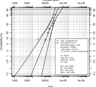
Figure 1: Standard Weibull plot from the Weibull Toolkit. The curves are confidence bounds. The middle (straight) line is the Median Rank Regression (MRR) fitted line, representing the two Weibull parameters β and η .
6 B-life
When the Weibull plot is created, predictions of the failure behaviour of the population of specimens can be made.
Weibull plot Age Unreliability [%] 1000 5000 50000 5e+05 5e+06 1000 5000 50000 5e+05 5e+06 0.1 0.5 1 2 5 10 20 50 90 99 0.1 0.5 1 2 5 10 20 50 90 99 (Age ; Unreliability [%]) curve (MRR, X on Y) beta (shape,slope) = 2.581 eta (scale) = 132500 n (fail | susp.) = 8 (8 | 0) r^2 | CCC^2 = 0.9375 | 0.8425 (good) CI = 90 [%] lower CB = 5 [%] higher CB = 95 [%] R = 1000 B10 = NA | 55420 B1 = NA | 22300 B0.1 = NA | 9123 B0.01 = NA | 3738
The B-life is the age at which a certain percentage of the population under investigation is expected to fail. For example, the B10-life for our population of engine mounts is 55420. The B0.1-life is 9123. Just draw a horizontal line at the 10 [%] resp. 0.1 [%] unreliability level and find the intersection with the fitted (straight) line. Then, read the age from the horizontal axis.
6.1 Confidence in predicted B-lives
For a sample of observations with calculated β and η, a 5 [%] lower confidence bound for B-lives has the following meaning:
“The real, unknown B-life of the specimens will, with a 5 [%] frequency, be smaller than the given B-life at the 5 [%] confidence bound. So this means that, with a 95 [%] frequency, the real, unknown B-life exceeds the B-life at the 5 [%] confidence bound).”
In the provided example, the B10 life is approximately 26000 with 95 [%] confidence level, the B0.1 life is only 1140 with 95 [%] confidence level (the number following the capital ‘B’ indicates the unreliability percentage). By using confidence bounds one is able to make reliable predictions based on a very small sample set; but it is clear that these bounds will be so wide that the resulting B-lives will be so small that they are of little practical use. Testing more specimens will narrow the confidence bounds.
In the automotive industry, a confidence level of 50 [%] is often used. Actually, this means that they do not use confidence bounds at all but read their B-lives straight from the fitted line. In these cases they trust that testing a ‘sufficient’ amount of specimen compensates for the lack of confidence. Much higher confidence levels are used (90 [%] to 99.9 [%] or more) in the medical and aircraft industry.
Confidence bounds are a key point where commercial software packages differ in implementations and availability. While ‘Beta Binomial Bounds’ (the dotted lines in fig. 1) are generated by an simple formula, others are more complex or use Monte Carlo simulations (e.g. ‘Pivotal Confidence Bounds’ using Monte
Carlo simulation). Discussion of the generation of these confidence bounds is beyond the scope of this article, check out ref. [2] for a more detailed treatment.
7 Conclusion
The commonly used Weibull model and its usage in fatigue and reliability analysis are introduced in this article. The authors explained the reasons to create their own analysis software, providing unique insights in the inner workings, strengths and weaknesses of commercial software. The toolkit is written for the statistical programming language R, ensuring minimal programming effort is needed to create powerful software.
The Weibull toolkit is constantly under active development, features are added and the code is being streamlined. It is available under a GPL3 license, making it Open Source software, so anyone can participate in the development. Ultimately, the Weibull toolkit will serve as a training tool for better understanding Weibull analysis and lifetime modelling in general, and for learning the proper usage of the commercial software tools.
8 References
[1] http://mechanics.kahosl.be/fatimat/inde
x.php/downloads-and-information/40/171
download area from the FATIMAT project’s website with the most recent version of this document.
[2] ‘The Weibull model in fatigue and
reliability analysis: an introduction &
implementations in R’ (Jurgen
Symynck – Filip De Bal – KaHo Sint-Lieven – 2010)
http://mechanics.kahosl.be/fatimat/inde
x.php/downloads-and-information/40/77
in-depth treatment of the subject of this article.
[4] http://www.kahosl.be/site/index.php?p =/nl/page/153/
homepage of the PWO funding channel on the website of KaHo Sint-Lieven. [5] http://www.kahosl.be [6] http://www.reliasoft.com [7] http://www.barringer1.com/wins.htm [8] • http://mechanics.kahosl.be/fati mat/index.php/multimedia/36/1 93 • http://www.youtube.com/watc h?v=g2IczVyuQkQ
Video clip of an experimental servopneumatic fatigue test bench.
[9] ‘A Comparison Between The Weibull
And Lognormal Models Used To
Analyse Reliability Data.’ (Mr.
Chi-Chao Lui, PhD 1997, dissertation from University of Nottingham) [10] http://www.r-project.org/ [11] http://cran.r-project.org/ [12] http://www.sciviews.org/Tinn-R/ [13] http://sourceforge.net/projects/weibullt oolkit/ [14] http://weibulltoolkit.git.sourceforge.net /git/gitweb-index.cgi [15] http://git-scm.com/ [16] http://code.google.com/p/msysgit/ [17] http://cran.r-project.org/web/packages/survival/ 9 Notes
9.1 Installing the toolkit under Windows
1) Go to the Weibulltoolkit’s homepage on Sourceforge.net (ref. [13]) and
download the toolkit package, named
weibulltoolkit_0.1.6.zip. 2) For simplicity of these instructions,
move the zip file to c:\temp. 3) Open the R console and type at the
prompt:
install.packages("c:/temp/weibulltoolkit_0.1.6. zip",repos=NULL)
... resulting in the successful installation of the toolkit.
Check the toolkit by typing the following code at the prompt, resulting in the execution of some demo routines:
library(weibulltoolkit) demo(weibulltoolkit)
You can get help on the toolkit’s main function by entering ?plot.wb at the prompt.
9.2 Code compatibility
Because the toolkit is under perpetual heavy development, currently the examples in this article that make use of the Weibull toolkit are only guaranteed to work using the toolkit
with version number 0.1.6
(weibulltoolkit_0.1.6.tar.gz or
weibulltoolkit_0.1.6.zip). When downloading the source code using GIT, go to the projects website to find instructions on identifying compatible code.